Computing Extremal Quasiconformal Maps - Technion

More documents

Recommendations

Info

O. Weber & A. Myles & D. Zorin / Computing Extremal Quasiconformal Maps Teichmüller maps. Locally in a neighborhood of every point (excluding zeros of gz), a Teichmüller map has the form (3): h◦Ak ◦g, for a choice of conformal maps h(w) and g(z), where w denotes the complex coordinate on the intermediate domain Ak acts on. A simple calculation leads to the following lemma: Lemma 1 For a map f = h ◦ Ak ◦ g, where h and g are conformal, and Ak is a stretch with dilatation k, the Beltrami coefficient has the form where φ = (gz) 2 . f¯z fz = k ¯φ |φ| Proof By Cauchy-Riemann equations, h ¯w = 0, and g¯z = 0; similarly, for the anti-conformal map ¯g, ¯gz = 0. Observe that the affine map Ak(w) in complex form can be written as Ak(w) = w + k ¯w. For this reason, fz = hw(gz + k ¯gz) = hwgz, and f¯z = hw(g¯z +k ¯g¯z) = khw ¯g¯z (because g is conformal, g¯z = 0 and ¯gz = 0). We observe that f¯z/ fz = k ¯g¯z/gz = kgz 2 /|g 2 z |, as ¯g¯z = gz. source Ak stretch h target g Figure 4: Locally, a Teichmüller map can be decomposed into two conformal maps and an affine transform. The quantity φ = g 2 z is called the quadratic differential of f . Geometrically, the quadratic differential can be interpreted, up to a scale, as the traceless part of the metric tensor M = J[ f ] ⊤ J[ f ] of the map f , where J[ f ] is the Jacobian matrix. More specifically, the singular vectors of A(φ(z)) determine the stretch directions of f at z. More generally, a quadratic differential on a domain with a complex coordinate z is defined by a holomorphic function φ(z), which depends on the choice of the coordinate system. If w is a different choice of complex coordinates on the domain, then φ w (w)w 2 z = φ(z). This change-of-coordinates rule also allows to define a quadratic differential on a Riemann surface by a set of holomorphic functions on local charts. Definition 1 On a planar domain D, a map f is called a Teichmüller map, if it is quasiconformal with Beltrami coefficient of the form µ(z) = k φ(z) |φ(z)| where φ is a holomorphic function and k is a constant dilatation, everywhere where φ = 0. (4) Observe that the definition is invariant with respect to composition with conformal maps on either side. While postcomposition does not change the Beltrami coefficient, precomposition results in a change in φ but not in k. Unlike the definition of extremal quasiconformal maps, involving minimization of a nonsmooth and nonlinear functional, Teichmüller maps are much more amenable to computation, thanks to explicit form of the Beltrami coefficient. Fortunately, in most cases, an extremal map is a Teichmüller map and it is unique. In particular, the following proposition can be obtained from a sufficient condition for Teichmüller map existence for disks [Rei02] and conformal mapping properties: Proposition 2 For two simply connected bounded domains D and D ′ with piecewise smooth boundaries forming nondegenerate corners; suppose h : ∂D → ∂D ′ is a function with continuous nonvanishing bounded derivative and almost everywhere defined second derivative. Then in every homotopy class of maps f satisfying f | ∂D = h, there is a unique extremal Teichmüller map f with bounded L1-norm of the quadratic differential φ. As illustrated in Figure 3, the conditions on h in proposition 2 are essential. The quasiconformal map of the disk to itself shown in this image is known to be extremal for its boundary values [Rei02]. The map in the image is obtained as f2 ◦ g ◦ f1, where f1(z) = i(1 + z)/(1 − z) maps the disk to the upper half-plane, f2 is its inverse, and g(z) = |z|z, and can be easily shown not to be a Teichmüller map. A similar statement appears to hold for multiply connected domains [Gar], but we were unable to locate a published proof. These theorems extend immediately to surfaces of genus zero with boundary, and also hold for maps between surfaces of arbitrary finite genus. In this paper, we focus on genus zero. Proposition 2 is the foundation of our approach for the computation of extremal maps. For these types of boundary data, it is sufficient to find a map with holomorphic quadratic differential and constant dilatation. Quadratic differential structure. Before discussing the algorithm we briefly mention the local structure of quadratic differentials near its zeros and poles. The quadratic differentials of Teichmüller maps have only simple poles, and generically zeros of order 1. The trajectories of quadratic differentials are integral lines of the fields of singular directions of A(φ(z)). These directions change rapidly near zeros and poles, as can be seen in Figure 5. While poles of quadratic differentials always remain on the boundaries, zeros spontaneously appear in the interior or on the boundary (Figure 9). 4. Algorithm Overview. Given a boundary function fb and an initial (not necessarily bijective) map satisfying boundary conditions, we compute a piecewise-linear approximation to a Teichmüller map minimizing a discretization of the least-squares Beltrami (LSB) energy: ELSB = D f¯z − k ¯φ |φ| fz 2 dA (5) c○ 2012 The Author(s) c○ 2012 The Eurographics Association and Blackwell Publishing Ltd.
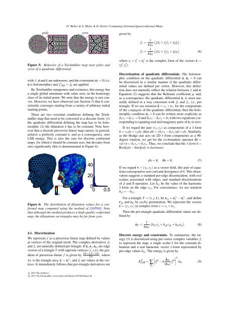
pole zero O. Weber & A. Myles & D. Zorin / Computing Extremal Quasiconformal Maps Figure 5: Behavior of a Teichmüller map near poles and zeros of a quadratic differential. with f , φ and k are unknowns, and the constraints φ¯z = 0 (i.e. φ is holomorphic) and f | ∂D = fb are applied. By Teichmüller uniqueness and existence, this energy has a single global minimum with value zero, in the homotopy class of its initial point. We note that the energy is not convex. However, we have observed (see Section 5) that it consistently converges starting from a variety of arbitrary initial starting points. There are two essential conditions defining the Teichmüller map that need to be converted to a discrete form: (1) the quadratic differential defining the map has to be holomorphic (2) the dilatation k has to be constant. Note however that a discrete piecewise-linear map cannot, in general, achieve a perfectly constant k, and as a consequence, zero LSB energy. This is also the case for discrete conformal maps, for which k should be constant zero, but deviates from zero significantly (this is demonstrated in Figure 6). 0.1 0 40 20 0 0 0.5 Figure 6: The distribution of dilatation values for a conformal map computed using the method of [SSP08]. Note that although the method produces a high-quality conformal map, the dilatations on triangles may be far from zero. 4.1. Discretization We represent f as a piecewise-linear map defined by values at vertices of the original mesh. The complex derivatives f¯z and fz are naturally defined per triangle. If ei,ej,ek, are edge vectors of a triangle T with opposite vertices (i, j,k), the gra- fiti+ f jt j+ fktk dient of piecewise-linear f is given by , where 2AT AT is the triangle area, ti = e ⊥ i , and fi are values at the vertices. It immediately follows that per-triangle derivatives are c○ 2012 The Author(s) c○ 2012 The Eurographics Association and Blackwell Publishing Ltd. given by fz = 1 fi 4AT ¯ti + f j ¯ f¯z = 1 4AT t j + fk ¯ tk , fiti + f jt j + fktk where ti = t x i + it y i is the complex form of the vectors ti = (t x i ,t y i ). Discretization of quadratic differentials. The holomorphic condition on the quadratic differential φ, φ¯z = 0 can be discretized in a similar manner if the quadratic differential values are defined per vertex. However, this definition does not naturally reflect the relation between f and φ. Equation (2) suggests that the Beltrami coefficient µ, and, as a consequence, the quadratic differential φ, is most naturally defined in a way consistent with f¯z and fz, i.e., per triangle. If we use notation ¯φ = vx + ivy for the components of the conjugate of the quadratic differential, then the holomorphic condition φ¯z = 0 can be written more explicitly as ∂xvx +∂yvy = 0 and ∂yvx −∂yvy = 0, with two equations corresponding to equating real and imaginary parts of φ¯z to zero. If we regard the pair (vx,vy) as components of a 1-form h = vxdx + vydy, then dh = (∂yvx − ∂xvy)dx ∧ dy. Similarly, as the Hodge star acts on 2D 1-form components as a 90degree rotation, we get for the co-boundary operator δh = ∗d ∗ h = ∂xvx + ∂yvy. Thus, we conclude that the 1-form h = Re(φ)dx − Im(φ)dy is harmonic: (6) dh = 0, δh = 0. (7) If we regard v = (vx,vy) as a vector field, this pair of equations correspond to zero curl and divergence of v. This observation suggests a standard per-edge discretization, with real scalars associated with edges, and standard discretizations of d and δ operators. Let hi j be the value of the harmonic 1-form on the edge ei j. For convenience, we use notation h ji = −hi j. For a triangle T = (i, j,k), let ri j = e ⊥ j − e ⊥ i , and define r jk and rki by cyclic permutation. We represent the vectors r = (rx,ry) in complex form r = rx + iry. Then the per-triangle quadratic differential values are defined by φT = 1 hi jri j + h jkr jk + hkirki . (8) 6AT Discrete energy and constraints. To summarize, the energy (5) is discretized using per-vertex complex variables fi to represent the map, a single scalar k for the constant dilatation and a real harmonic vector 1-form represented by per-edge values hi j. The energy is given by E d LSB = ∑ Tm f m ¯z − k ¯φm |φm| f m 2 z Am (9)
Page 1 and 2: Eurographics Symposium on Geometry
Page 3: O. Weber & A. Myles & D. Zorin / Co
Page 7 and 8: O. Weber & A. Myles & D. Zorin / Co
Page 9 and 10: 0.7 0.4 0.1 O. Weber & A. Myles & D
Page 11: O. Weber & A. Myles & D. Zorin / Co

Computing Extremal Quasiconformal Maps - Technion

Create successful ePaper yourself

Delete template?

Save as template?