Computing Extremal Quasiconformal Maps - Technion

More documents

Recommendations

Info

O. Weber & A. Myles & D. Zorin / Computing Extremal Quasiconformal Maps with φ defined by (8), and fz and f¯z defined by (6). Additional constraints ensure that h is harmonic: hi j + h jk + hki = 0,for triangle T = (i, j,k) ∑wi jhi j = 0,for a vertex j, j (10) where wi j are the standard cotangent weights, with the two conditions corresponding to vanishing boundary and coboundary operators d and δ. We introduce an auxiliary variable sm = 1/|φm|. With this variable, the energy takes the form E d LSB = ∑ Tm m f¯z − k¯φmsm f m z 2 Am (11) with an additional nonlinear constraint sm = 1/|φm|. While we focus on Dirichlet boundary conditions defined on the whole boundary, we note that free boundaries can be easily added. 4.2. Optimization The energy (9) is highly nonlinear. Standard methods for optimizing this energy that we have tried (quasi-Newton methods) do not behave well (see Section 5). At the same time, the energy is quadratic with respect to each of the vector variables f = [ f1,... fP] and h = [h1,...hL] where P and L are the number of vertices and edges respectively. It is also quadratic with respect to the global variable k. The nonlinearity in the solution reduces to enforcing the constraint between sm and φm. This observation suggests an alternating-descent algorithm, with h, f and k minimized in alternating fashion. While this does not guarantee convergence to a global minimum, this yields a stable algorithm with consistent practical behavior (See Section 5). If f, h are fixed, k can be easily computed explicitly. Furthermore, for fixed f, we use the following property of the energy: Proposition 3 For fixed f, optimal discrete holomorphic φ (up to a scale factor) does not depend on k, and optimal k is given by Re(ˆµm f k = ∑2Am m m ¯z ) ∑m Am| f m ¯z |2 (12) where ˆµm = ¯φm . This formula is easily obtained by direct |φm| computation. The algorithm in its basic form (Algorithm 1) alternates two steps. We use a harmonic f to initialize the iterative solution, corresponding to minimizing LSB energy with constant k = 0. In the main loop, a quadratic problem is solved to determine an optimal value h new , keeping f and s fixed, in general violating the nonlinear constraint sm = 1/|φm|. The constraint is enforced by projection, and a line search is performed in the direction determined by h new , to ensure that the energy decreases. The stability of this algorithm is guaranteed as the energy is forced to decrease at each step; boundary conditions are also satisfied by construction. Its main limitation is that Algorithm 1 Initialize f to harmonic, sm to 1. Initialize h := argmin h E d LSB (h,f,s,1) Initialize k using Equation 12 while energy change > ε f do while energy change > εφ do {Optimize h for fixed f, k and s.} h new := argmin h E d LSB (h,f,s,k) {Perform 1-dimensional search on the line between h and h new } t opt = argmin t E d LSB ((1 −t)h +thnew ,f,s(t),k) h := (1 −t opt )h +t opt h new Compute k using Equation 12. end while {Optimize f for fixed h, k and s} f := argmin f E d LSB (h,f,s,k) end while there is no guarantee that the global minimum is reached or approximated well. In practice, we observe that the algorithm converges to the same solution, even for large variations in the starting point; furthermore, in all our test cases for which the global minimum is known, the algorithm converges to this global minimum, as discussed in more detail in Section 5. Extension to surfaces. The algorithm directly extends to mapping genus-zero surfaces with boundary to the plane. Because quasiconformal distortion is conformally invariant, it is sufficient to use an arbitrary conformal map of the surface to the plane, and the composition of this conformal map with the computed extremal quasiconformal map is extremal. We use the scale-factor based conformal map computation to map surfaces to the plane [BGB08, SSP08]. Specifically, for a multiply connected domain of genus zero we follow these steps: • One boundary is chosen as external; the remaining boundary loops are triangulated, reducing the surface to simply connected. • The algorithm of [SSP08] is used to compute a logarithmic scale factor ui for each vertex ui, such that edge lengths li j = e (ui+u j)/2 define a planar mesh. For the solution to be unique, we choose the scale factors to be zero on the outer boundary (i.e., no scale distortion along the boundary). • The added triangles are removed to obtain the discrete conformal image of the original mesh. We note that the metric used for the conformal map need not coincide with the Euclidean embedding metric. This can be used for minimizing different types of errors in the parametrization (cf. [KMZ10]), as well as “correction” of a non-bijective parametrization (i.e. nearly flat metric). If the metric is derived from a different locally bijective parametrization, there is no need for the flattening conformal map; however if the parametrization is not locally bijective, the conformal map is still needed. Figure 18 shows some examples of this. c○ 2012 The Author(s) c○ 2012 The Eurographics Association and Blackwell Publishing Ltd.
O. Weber & A. Myles & D. Zorin / Computing Extremal Quasiconformal Maps Discussion. By construction, the quadratic differential computed by the algorithm is discrete holomorphic and the corresponding Beltrami coefficient has constant dilatation k. At the same time, the actual Beltrami coefficient of the map f¯z/ fz is just an approximation to the “perfect” computed coefficient. We note that in general, if ˆµ (i.e. the angular part of µ) is fixed, this determines the parametrization uniquely with no control for k on each triangle. While we observe good convergence of the algorithm to constant k in L 2 norm when the mesh is refined, this does not guarantee that k < 1 (i.e. there are no fold-overs) on all triangles, even for a very fine mesh. In practice, we observe that no triangles are flipped for a sufficiently fine mesh, excluding few triangles near highly concave parts of the boundary. In the next section, we present a detailed evaluation of the behavior of the algorithm: dependency on the starting point, convergence rates, comparison to analytic cases. 5. Evaluation Validation. We validate our method in several ways. The most direct validation is comparison to analytically computed maps. Unfortunately, the analytic solution is known explicitly only in few cases. We consider two maps known analytically: mapping a disk to itself with four boundary points moved to different locations, and mapping of a ring to a ring with a different ratio of inner to outer radius. In the first case, we consider maps moving points at angular locations ±π/4,π ± π/4 on a circle, to ±φ,π ± φ. This map is given by fφ(z) = e −iφ F ze iφ ,e −2iφ where F(z,w) is the incomplete elliptic integral of the first kind. For the ring domain with inner and outer radii r0 and r1, mapped to a ring with inner and outer radii r ′ 0 and r′ 1 , the extremal map has the polar coordinate form (r,φ) → (r ′ 0(r/r0) K ,φ) where K = ln(r ′ 1 /r′ 0 )/ln(r1/r0). In both cases, we observe an accurate match both for the maps, and extremal dilatation values. We can also compute a subclass of Teichmüller maps semi-analytically, by prescribing a pair of conformal maps, and a stretch in the intermediate domain. 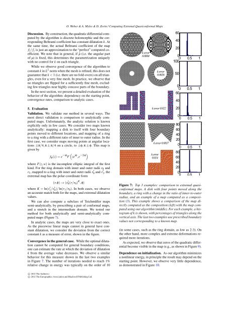We tested our method for both analytically and semi-analytically computed maps (Figure 7). In analytic cases, the maps are very close to exact ones. As the piecewise linear maps cannot in general have constant dilatation, we consider the deviation from the correct constant k as a measure of error, shown in the figure. Convergence in the general case. While the optimal dilatation cannot be computed for general boundary conditions, one can estimate the rate at which the deviation of dilatation k from the average value decreases. We observe a similar behavior for this measure shown in the last two examples in Figure 7. The number of iterations needed to reach 1% relative change in energy was typically on the order of 10 c○ 2012 The Author(s) c○ 2012 The Eurographics Association and Blackwell Publishing Ltd. k error 0.0004 k error 0.022 k error 0.0037 k error 0.014 k error 0.0026 60 40 20 0 0 0.5 1 100 50 0 0 60 0.5 1 40 20 0 0 0.5 1 80 60 40 20 0 0 80 60 40 20 0.5 1 0 0 0.5 1 Figure 7: Top 3 examples: comparison to extremal quasiconformal maps. A disk with four points moved along the boundary, a ring with a change in the ratio of inner-to-outer radius, and an example of a map computed as a composition (3). This example shows a comparison of the map directly computed as the composition (left) with the map computed using our algorithm (middle). For each example, a histogram of k is shown, with percentages of triangles along the vertical axis. The last two examples use prescribed boundary values not corresponding to a known map. (in some cases, such as the ring domain, as low as 2-3). On the other hand, more complex and extreme deformations required more iterations. As expected, we observe that zeros of the quadratic differential become visible in the map (e.g., as shown in Figure 9). Dependence on initialization. As our algorithm minimizes a nonlinear energy, in principle the result may depend on the starting point. However, we observe very little dependence, as demonstrated in Figure 10.
Page 1 and 2: Eurographics Symposium on Geometry
Page 3 and 4: O. Weber & A. Myles & D. Zorin / Co
Page 5: pole zero O. Weber & A. Myles & D.
Page 9 and 10: 0.7 0.4 0.1 O. Weber & A. Myles & D
Page 11: O. Weber & A. Myles & D. Zorin / Co

Computing Extremal Quasiconformal Maps - Technion

You also want an ePaper? Increase the reach of your titles

Delete template?

Save as template?