Primordial non-Gaussianity in the cosmological perturbations - CBPF

Abstract
Primordial non-Gaussianity
in the cosmological perturbations
Antonio Riotto
Département de Physique Théorique, Université de Genève,
24 quai Ansermet, CH-1211, Genève, Switzerland
This set of notes have been written down as supplementary material for the course on primordial
non-Gaussianity in the cosmological perturbations at the II Jayme Tiomno School of Cosmology held
at Brazilian Center for Research in Physics in Rio de Janeiro from 6 -10 August, 2012. Hopefully
they are self-contained, but by no means they are intended to substitute any of the reviews on the
subject. The notes contain some extended introductory material and a set of exercises, whose goal is
to familiarize the students with the basic notions necessary to deal with the issue of non-Gaussianity
in the cosmological perturbations.
email: Antonio.Riotto@unige.ch, phone: +41 22 379 6310 August 7, 2012
1

Literature
During the preparation of this set of notes, we have been found useful consulting the following
reviews and textbooks:
N. Bartolo, E. Komatsu, S. Matarrese and A. Riotto, “Non-Gaussianity from inflation: Theory and
observations,” Phys. Rept. 402, 103 (2004). [astro-ph/0406398];
X. Chen, “Primordial Non-Gaussianities from Inflation Models,” Adv. Astron. 2010, 638979 (2010)
[arXiv:1002.1416 [astro-ph.CO]];
V. Desjacques and U. Seljak, “Primordial non-Gaussianity in the large scale structure of the Uni-
verse,” Adv. Astron. 2010 (2010) 908640 [arXiv:1006.4763 [astro-ph.CO]];
S. Dodelson, “Modern Cosmology”, Academic Press, 2003;
J.A. Peacock, “Cosmological Physics”, Cambridge University Press, 1999.
Units
We will adopt natural, or high energy physics, units. There is only one fundamental dimension,
energy, after setting = c = kb = 1,
[Energy] = [Mass] = [Temperature] = [Length] −1 = [Time] −1 .
The most common conversion factors and quantities we will make use of are
1 GeV −1 = 1.97 × 10 −14 cm=6.59 × 10 −25 sec,
1 Mpc= 3.08×10 34 cm=1.56×10 33 GeV −1 ,
MPl = 1.22 × 10 19 GeV,
H0= 100 h Km sec −1 Mpc −1 =2.1 h × 10 −42 GeV −1 ,
ρc = 1.87h 2 · 10 −29 g cm −3 = 1.05h 2 · 10 4 eV cm −3 = 8.1h 2 × 10 −47 GeV 4 ,
T0 = 2.75 K=2.3×10 −13 GeV,
Teq = 5.5(Ω0h 2 ) eV,
Tls = 0.26 (T0/2.75 K) eV.
2

Contents
I Introduction 6
1 The Friedmann-Robertson-Walker metric 8
1.1 Open, closed and flat spatial models . . . . . . . . . . . . . . . . . . . . . . . . . . . 10
1.2 The particle horizon and the Hubble radius . . . . . . . . . . . . . . . . . . . . . . . 13
1.3 Particle kinematics of a particle . . . . . . . . . . . . . . . . . . . . . . . . . . . . . . 15
1.4 The cosmological redshift . . . . . . . . . . . . . . . . . . . . . . . . . . . . . . . . . 16
2 Standard cosmology 18
2.1 The stress-energy momentum tensor . . . . . . . . . . . . . . . . . . . . . . . . . . . 18
2.2 The Friedmann equations . . . . . . . . . . . . . . . . . . . . . . . . . . . . . . . . . 20
2.3 Exact solutions of the Friedman-Robertson-Walker Cosmology . . . . . . . . . . . . 23
II Equilibrium thermodynamics 28
3 Entropy 32
III The inflationary cosmology 34
4 Again on the concept of particle horizon 35
5 The shortcomings of the Standard Big-Bang Theory 36
5.1 The Flatness Problem . . . . . . . . . . . . . . . . . . . . . . . . . . . . . . . . . . . 36
5.2 The Entropy Problem . . . . . . . . . . . . . . . . . . . . . . . . . . . . . . . . . . . 37
5.3 The horizon problem . . . . . . . . . . . . . . . . . . . . . . . . . . . . . . . . . . . . 38
6 The standard inflationary universe 45
6.1 Inflation and the horizon Problem . . . . . . . . . . . . . . . . . . . . . . . . . . . . 46
6.2 Inflation and the flateness problem . . . . . . . . . . . . . . . . . . . . . . . . . . . . 47
6.3 Inflation and the entropy problem . . . . . . . . . . . . . . . . . . . . . . . . . . . . 49
6.4 Inflation and the inflaton . . . . . . . . . . . . . . . . . . . . . . . . . . . . . . . . . 49
6.5 Slow-roll conditions . . . . . . . . . . . . . . . . . . . . . . . . . . . . . . . . . . . . . 50
6.6 The last stage of inflation and reheating . . . . . . . . . . . . . . . . . . . . . . . . . 53
6.7 A brief survey of inflationary models . . . . . . . . . . . . . . . . . . . . . . . . . . . 56
6.7.1 Large-field models . . . . . . . . . . . . . . . . . . . . . . . . . . . . . . . . . 56
3

6.7.2 Small-field models . . . . . . . . . . . . . . . . . . . . . . . . . . . . . . . . . 57
6.7.3 Hybrid models . . . . . . . . . . . . . . . . . . . . . . . . . . . . . . . . . . . 58
IV Inflation and the cosmological perturbations 59
7 Quantum fluctuations of a generic massless scalar field during inflation 62
7.1 Quantum fluctuations of a generic massless scalar field during a de Sitter stage . . . 62
7.2 Quantum fluctuations of a generic massive scalar field during a de Sitter stage . . . 65
7.3 Quantum to classical transition . . . . . . . . . . . . . . . . . . . . . . . . . . . . . . 66
7.4 The power spectrum . . . . . . . . . . . . . . . . . . . . . . . . . . . . . . . . . . . . 66
7.5 Quantum fluctuations of a generic scalar field in a quasi de Sitter stage . . . . . . . 67
8 Quantum fluctuations during inflation 69
8.1 The metric fluctuations . . . . . . . . . . . . . . . . . . . . . . . . . . . . . . . . . . 71
8.2 Perturbed affine connections and Einstein’s tensor . . . . . . . . . . . . . . . . . . . 73
8.3 Perturbed stress energy-momentum tensor . . . . . . . . . . . . . . . . . . . . . . . . 76
8.4 Perturbed Klein-Gordon equation . . . . . . . . . . . . . . . . . . . . . . . . . . . . . 77
8.5 The issue of gauge invariance . . . . . . . . . . . . . . . . . . . . . . . . . . . . . . . 78
8.6 The comoving curvature perturbation . . . . . . . . . . . . . . . . . . . . . . . . . . 82
8.7 The curvature perturbation on spatial slices of uniform energy density . . . . . . . . 83
8.8 Scalar field perturbations in the spatially flat gauge . . . . . . . . . . . . . . . . . . . 84
8.9 Comments about gauge invariance . . . . . . . . . . . . . . . . . . . . . . . . . . . . 85
8.10 Adiabatic and isocurvature perturbations . . . . . . . . . . . . . . . . . . . . . . . . 85
8.11 The next steps . . . . . . . . . . . . . . . . . . . . . . . . . . . . . . . . . . . . . . . 87
8.12 Computation of the curvature perturbation using the longitudinal gauge . . . . . . . 88
8.13 A proof of time-independence of the comoving curvature perturbation for adiabatic
modes: linear level . . . . . . . . . . . . . . . . . . . . . . . . . . . . . . . . . . . . . 91
8.14 A proof of time-independence of the comoving curvature perturbation for adiabatic
modes: linear level . . . . . . . . . . . . . . . . . . . . . . . . . . . . . . . . . . . . . 92
8.15 A proof of time-independence of the comoving curvature perturbation for adiabatic
modes: all orders . . . . . . . . . . . . . . . . . . . . . . . . . . . . . . . . . . . . . . 94
9 Comoving curvature perturbation from isocurvature perturbation 96
9.1 Gauge-invariant computation of the curvature perturbation . . . . . . . . . . . . . . 99
10 Transferring the perturbation to radiation during reheating 103
11 The initial conditions provided by inflation 106
4

12 Symmetries of the de Sitter geometry 109
12.1 Killing vectors of the de Sitter space . . . . . . . . . . . . . . . . . . . . . . . . . . . 112
13 Non-Gaussianity of the cosmological perturbations 114
13.1 The generation of non-Gaussianity in the primordial cosmological perturbations: generic
considerations . . . . . . . . . . . . . . . . . . . . . . . . . . . . . . . . . . . . . . . . 117
13.2 A brief Review of the in-in formalism . . . . . . . . . . . . . . . . . . . . . . . . . . . 118
13.3 The shapes of non-Gaussianity . . . . . . . . . . . . . . . . . . . . . . . . . . . . . . 121
13.4 Theoretical Expectations . . . . . . . . . . . . . . . . . . . . . . . . . . . . . . . . . . 124
13.4.1 Single-Field Slow-Roll Inflation . . . . . . . . . . . . . . . . . . . . . . . . . . 124
13.4.2 Models with Large Non-Gaussianity . . . . . . . . . . . . . . . . . . . . . . . 127
13.4.3 Multiple Fields . . . . . . . . . . . . . . . . . . . . . . . . . . . . . . . . . . . 128
13.4.4 A test of multi-field models of inflation . . . . . . . . . . . . . . . . . . . . . . 131
13.4.5 Non-Standard Vacuum . . . . . . . . . . . . . . . . . . . . . . . . . . . . . . . 132
V The impact of the non-Gaussianity on the CMB anisotropies132
13.5 Why do we expect NG in the cosmological perturbations? . . . . . . . . . . . . . . . 134
13.6 Primordial non-Gaussianity and the CMB anisotropies . . . . . . . . . . . . . . . . . 138
13.7 Non-Gaussianity in the CMB anisotropies at recombination in the squeezed limit . . 145
VI Matter perturbations 148
14 Spherical collapse 153
15 The dark matter halo mass function and the excursion set method 158
15.1 The computation of the halo mass function as a stochastic problem . . . . . . . . . . 159
16 The bias 165
VII The impact of the non-Gaussianity on the halo mass function
167
VIII The impact of the non-Gaussianity on the halo clustering172
IX Exercises 177
5

Part I
Introduction
Our current understanding of the evolution of the universe is based upon the Friedmann-Robertson-
Walker (FRW) cosmological model, or the hot big bang model as it is usually called. The model is
so successful that it has become known as the standard cosmology. times. The FRW cosmology is
so robust that it is possible to make sensible speculations about the universe at times as early as
10 −43 sec after the Big Bang.
The most important feature of our universe is its large scale homogeneity and isotropy. This
feature ensures that observations made from our single point are representative of the universe as a
whole and can therefore be legitimately used to test cosmological models. For most of the twentieth
century, the homogeneity and isotropy of the universe had to be taken as an assumption, known as
the Cosmological Principle. The assumption of isotropy and homogeneity dates back to the earliest
work of Einstein, who made the assumption not based upon observations, but as theorists often do,
to simplify the mathematical analysis. The Cosmological Principle remained an intelligent guess
until firm empirical data, confirming large scale homogeneity and isotropy, were finally obtained
at the end of the twentieth century. The best evidence for the isotropy of the observed universe
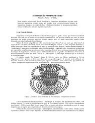
Figure 1: The large-scale structure from the 2dF Galaxy Survey
is the uniformity of the temperature of the cosmic microwave background (CMB) radiation: aside
from the observed dipole anisotropy, the temperature difference between two antennas separated by
angles ranging from about 10 arc seconds to 180 ◦ is smaller than about one part in 10 5 . The simplest
interpretation of the dipole anisotropy is that it is the result of our motion relative to the cosmic rest
frame. If the expansion of the universe were not isotropic, the expansion anisotiopy would lead to a
temperature anisotiopy in the CMBR of similar magnitude. Likewise, inhomogeneities in the density
of the universe on the last scattering surface would lead to temperature anisotropies. In this iegard,
6

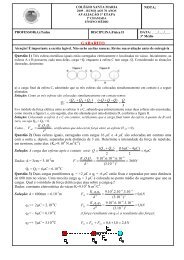
Figure 2: The CMB radiation projected onto a sphere
the CMBR is a very powerful probe: It is even sensitive to density inhomogeneities on scales larger
than our present Hubble volume. The remarkable uniformity of the CMB radiation indicates that
at the epoch of last scattering for the CMB radiation (about 200,000 yr after the bang) the universe
was to a high degree of precision (order of 10 −5 or so) isotropic and homogeneous. Homogeneity and
isotropy is of course true if the universe is observed at sufficiently large scales. The observable patch
of the universe is of order 3000 Mpc. Redshift surveys suggest that the universe is homogeneous
and isotropic only when coarse grained on scales of the order of 100 Mpc. On smaller scales there
exist large inhomogeneities, such as galaxies, clusters and superclusters. Hence, the Cosmological
Principle is only valid within a limited range of scales, spanning a few orders of magnitude. The
inflationary theory, as we shall see, suggests that the universe continues to be homogeneous and
isotropic over distances larger than 3000 Mpc.
It is firmly established by observations that our universe therefore
• is homogeneous and isotropic on scales larger than 100 Mpc and has well developed inhomo-
geneous structure on smaller scales;
• expands according to the Hubble law for which the recession velocity of, say, galaxies is
proportional to their distances.
Concerning the matter composition of the universe, we know that
• it is pervaded by thermal microwave background radiation with temperature T0 2.73 K;
7

• there is baryonic matter, roughly one baryon per 10 9 photons, but no substantial amount of
antimatter;
• the chemical composition of baryonic matter is about 75% hydrogen, 25% helium, plus trace
amounts of heavier elements;
• baryons contribute only a small percentage of the total energy density; the rest is a dark
component, which appears to be composed of cold dark matter with negligible pressure (25%)
and dark energy with negative pressure (70%).
Observations of the fluctuations in the cosmic microwave background radiation suggest that
• there were only small fluctuations of order 10 −5 in the energy density distribution when the
universe was a thousand times smaller than now.
Any cosmological model worthy of consideration must be consistent with established facts. While
the standard big bang model accommodates most known facts, a physical theory is also judged
by its predictive power. At present, inflationary theory, naturally incorporating the success of the
standard big bang, has no competitor in this regard. Therefore, we will build upon the standard big
bang model, which will be our starting point, until we reach contemporary ideas of inflation. We
will then show how its prediction influences the CMB physics as well as the physics of the matter
perturbations. This set of notes also offers two Appendices about the generation of the baryon
asymmetry of the universe and the phase transitions in the early universe. These subjects will not
be covered during the lectures.
1 The Friedmann-Robertson-Walker metric
As discussed in the previous section, the distribution of matter and radiation in the observable
universe is homogeneous and isotropic. While this by no means guarantees that the entire universe is
smooth, it does imply that a region at least as large as our present Hubble volume is smooth. So long
as the universe is spatially homogeneous and isotropic on scales as large as the Hubble volume, for
purposes of description of our local Hubble volume we may assume the entire universe is homogeneous
and isotropic. While a homogeneous and isotropic region within an otherwise inhomogeneous and
anisotropic universe will not remain so forever, causality implies that such a region will remain
smooth for a time comparable to its light-crossing time. This time corresponds to the Hubble time,
about 10 Gyr. We have determined during the last part of the GR course that the metric of a
maximally symmetric space satisfying the Cosmological Principle is the the metric for a space with
homogeneous and isotropic spatial sections, that is the Friedmann-Robertson-Walker metric, which
can be written in the form
8

ds 2 = −dt 2 + a 2
dr2 (t)
1 − kr2 + r2dθ 2 + r 2 sin 2 θdφ 2
, (1)
where (t, r, θ, φ) are are coordinates (referred to as comoving coordinates), a(t) is the cosmic scale
factor, and with an appropriate reseating of the coordinates, k can be chosen to be +1, −1, or 0
for spaces of constant positive, negative, or zero spatial curvature, respectively. The coordinate r is
dimensionless, i.e. a(t) has dimensions of length, and r ranges from 0 to 1 for k = +1. The time
coordinate is just the proper (or clock) time measured by an observer at rest in the comoving frame,
i.e., (r, θ, φ)=constant. As we shall discover shortly, the term comoving is well chosen: observers at
rest in the comoving frame remain at rest, i.e., (r, θ, φ) remain unchanged, and observers initially
moving with respect to this frame will eventually come to rest in it. Thus, if one introduces a
homogeneous, isotropic fluid initially at rest in this frame, the t =constant hypersurfaces will always
be orthogonal to the fluid flow, and will always coincide with the hypersurfaces of both spatial
homogeneity and constant fluid density.
We already know the curvature tensor of the maximally symmetric metric entering the FRW
metric (and its contractions), this is not difficult.
1. First of all, we write the FRW metric as
ds 2 = −dt 2 + a 2 (t)gijdx i dx j . (2)
From now on, all objects with a tilde will refer to three-dimensional quantities calculated with
the metric gij.
2. One can then calculate the Christoffel symbols in terms of a(t) and Γi jk . The nonvanishing
components are (we had already established that Γ µ
00 = 0)
Γ i jk = Γ i jk ,
Γ i j0 = ˙a
a δi j,
3. The relevant components of the Riemann tensor are
Γ 0 ij = ˙a
a gij. (3)
R i 0j0 = − ä
a δi j,
R 0 i0j = äagij,
R k ikj = Rij + 2 ˙a 2 gij. (4)
9

4. Now we can use Rij = 2kgij (as a consequence of the maximally symmetry of gij) to calculate
Rµν. The nonzero components are
5. The Ricci scalar is
and
R00 = −3 ä
a ,
6. the Einstein tensor has the components
Rij = aä + 2 ˙a 2 + 2k gij,
ä ˙a2 k
= + 2 + 2
a a2 a2
gij. (5)
G0i = 0,
R = 6
a2 2
aä + ˙a + k , (6)
˙a 2
G00 = 3
Gij = −
k
+
a2 a2
2 ä
a
1.1 Open, closed and flat spatial models
,
˙a2 k
+ +
a2 a2
gij. (7)
In order to illustrate the construction of the metric, consider the simpler case of a two spatial
dimensions. dimensions. Examples of two-dimensional spaces that are homogeneous and isotropic
are the flat plane R 2 , the positively-curved closed two sphere S 2 and the negatively-curved hyperbolic
plane H 2 .
Consider first a two sphere S 2 of radius a and embedded in a three-dimensional space R 3 . The
equation of the sphere of radius a is
The element of length is the three-dimensional Euclidean space is
x 2 1 + x 2 2 + x 2 3 = a 2 . (8)
dx 2 = dx 2 1 + dx 2 2 + dx 2 3. (9)
Since x3 is a fictitious coordinate, we can eliminate it in favour of the other two and write
dx 2 = dx 2 1 + dx 2 2 + (x1dx1 + x2dx2) 2
a2 − x2 1 − x2 . (10)
2
10

Now, let us introduce the polar coordinates
in terms of which the infinitesimal line length becomes
x1 = r ′ cos θ, x2 = r ′ sin θ, (11)
dx 2 = a2 dr ′ 2
a 2 − r ′ 2 + r′ 2 dθ 2 . (12)
Finally, with the definition of a dimensionless coordinate r = r ′ /a (0 ≤ r ≤ 1), the spatial metric
becomes
dx 2 = a 2
dr2 1 − r2 + r2dθ 2
. (13)
Note the similarity between this metric and the k = 1 FRW metric. It should also now be clear that
a(t) is the radius of the space. The poles of the two-sphere are at r = 0, the equator is at r = 1.
The locus of points of constant r sweep out the latitudes of the sphere, while the locus of points of
constant θ sweep out the longitudes of the sphere. Another convenient coordinate system for the
two sphere is that specified by the usual polar and azimuthal angles (θ, φ) of spherical coordinates,
related to the xi by
x1 = a sin θ cos φ, x2 = a sin θ sin φ, x3 = a cos θ. (14)
In terms of these coordinates, the spatial line element becomes
dx 2 = a 2 dθ 2 + sin 2 θdφ 2 . (15)
This form makes manifest the fact that the space is the two sphere of radius a. The volume of the
two sphere is easily calculated
VS2 = d 2 2π π
g = dφ dθ a
0 0
2 sin 2 θ = 4πa 2 , (16)
as expected. The two sphere is homogeneous and isotropic. Every point in the space is equivalent
to every other point, and there is no preferred direction. In other words, the space embodies
the Cosmological Principle, i.e., no observer (especially us) occupies a preferred position in the
universe. Note that this space is unbounded; there are no edges on the two sphere. It is possible to
circumnavigate the two sphere, but it is impossible to fall off. Although the space is unbounded, the
volume is finite. The expansion (or contraction) of this two-dimensional universe equivalent to an
increase (or decrease) in the radius of the two sphere a. Since the universe is apatiatly homogeneous
and isotropic, the scale factor can only be a function of time. As the two sphere expands or contracts,
the coordinates (r and θ in the case of the two sphere) remain unchanged; they are “comoving.”
11

Also note that the physical distance between any two comoving points in the space scales with a
(hence the name scale factor).
The equivalent formulas for a space of constant negative curvature can be obtained with the
replacement a → ia. In this case the embedding is in a three-dimensional Minkowski space. The
metric corresponding to the form for the negative curvature case is
dx 2 = a 2
dr2 1 − r2 + r2dθ 2
= a 2 dθ 2 + sinh 2 θdφ 2 . (17)
The hyperbolic plane H 2 is unbounded with infinite volume since 0 ≤ θ < ∞. The embedding of
H 2 in a Euclidean space requires three fictitious extra dimensions, and such an embedding is of
little use in visualizing the geometry. The spatially-flat model can be obtained from either of the
above examples by taking the radius a to infinity. The flat model is unbounded with infinite volume.
For the flat model the scale factor does not represent any physical radius as in the closed case, or
an imaginary radius as in the open case, but merely represents how the physical distance between
comoving points scales as the space expands or contracts.
The generalization of the two-dimensional models discussed above to three spatial dimensions
is trivial. For the three sphere a fictitious fourth spatial dimension is introduced, and in cartesian
coordinates the three sphere is denned by: a 2 = x 2 1 + x2 2 + x2 3 + x2 4 . The spatial metric is dx2 =
dx2 1 + dx22 + dx23 + dx24 . The fictitious coordinate can be removed to give
dx 2 = dx 2 1 + dx 2 2 + dx 2 3
(x1dx1 + x2dx2 + x3dx3) 2
a2 − x2 1 − x22 − x2 . (18)
3
In terms of the coordinates x1 = r ′ sin θ cos φ, x2 = r ′ sin θ sin φ and x3 = r ′ cos θ, this metric
becomes equal to the FRW metric with k = +1 and r = r ′ /a. In the coordinate system that
employes the three angular coordinates (χ, θ, φ) of a four-dimensional spherical coordinates system,
x1 = a sin χ sin θ cos φ, x2 = a sin χ sin θ sin φ, x3 = a sin χ cos θ and x4 = a cos χ, the metric is given
by
The volume of the three-sphere is
dx 2 = a 2 dχ 2 + sin 2 χ(dθ 2 + sin 2 θdφ 2 ) . (19)
VS3 =
d 3 x g = 2πa 3 . (20)
As for the two-dimensional case, the three-dimensional open model is obtained by the replacement
a → ia, which gives the FRW metric with k = −1. Again the Again the space is unbounded with
infinite volume and a(t) sets the curvature scale. Embedding H 3 in a Euclidean space requires four
fictitious extra dimensions.
12

It should be noted that the assumption of local homogeneity and isotropy only implies that
the spatial metric is locally S 3 , H 3 or R 3 and the space can have different global properties. For
instance, for the spatially fiat case the global properties of the space might be that of the three torus,
T 3 , rather than R 3 ; this is accomplished by identifying the opposite sides of a fundamental spatial
volume element. Such non-trivial topologies may be relevant in light of recent work on theories with
extra dimensions. In many such theories the internal space (of the extra dimensions) is compact,
but with non-trivial topology, e.g., containing topological defects such as holes, handles, and so
on. If the internal space is not simply connected, it suggests that the external space may also be
non-trivial, and the global properties of our three-space might be much richer than the simple S 3 ,
H 3 or R 3 topologies.
1.2 The particle horizon and the Hubble radius
A fundamental question in cosmology that one might ask is: what fraction of the universe is in causal
contact? More precisely, for a comoving observer with coordinates (r0, θ0, φ0), for what values of
(r, θ, φ) would a light signal emitted at t = 0 reach the observer at, or before, time t? This can
be calculated directly in terms of the FRW metric. A light signal satisfies the geodesic equation
ds 2 = 0. Because of the homogeneity of space, without loss of generality we may choose r0 = 0.
Geodesies passing through r=0 are lines of constant θ and φ, just as great circles eminating from the
poles of a two sphere are lines of constant θ (i.e., constant longitude), so dθ = dφ = 0. Of course,
the isotropy of space makes the choice of direction θ0, φ0) irrelevant. Thus, a light signal emitted
from coordinate position (rH, θ0, φ0) at time t = 0 will reach r0 = 0 in a time t determined by
t
0
dt ′
a(t ′ ) =
rH
0
The proper distance to the horizon measured at time t is
t
RH(t) = a(t)
0
dt ′
a(t ′ a da
= a(t)
) 0
′
a ′
1
a ′ H(a ′ rH
= a(t)
) 0
dr ′
√ 1 − kr ′ 2 . (21)
dr ′
√ 1 − kr ′ 2 (PARTICLE HORIZON).
If RH(t) is finite, then our past light cone is limited by this particle horizon, which is the boundary
between the visible universe and the part of the universe from which light signals have not reached
us. The behavior of a(t) near the singularity will determine whether or not the particle horizon is
finite. We will see that in the standard cosmology RH(t) ∼ t, that is the particle horizon is finite.
The particle horizon should not be confused with the notion of Hubble radius
1
H
= a
˙a
(22)
(HUBBLE RADIUS). (23)
13

Let us emphasize a subtle distinction between the particle horizon and the Hubble: if particles are
separated by distances greater than RH(t) they never could have communicated with one another;
if they are separated by distances greater than the Hubble radius H −1 , they cannot talk to each
other at the time t.
We shall see that the standard cosmology the distance to the horizon is finite, and up to numerical
factors, equal to the Hubble radius, H −1 , but during inflation, for instance, they are drastically
different. One can also define a comoving particle horizon distance
t
τH =
0
dt ′
a(t ′ ) =
a da
0
′
H(a ′ )a ′ 2 =
a
0
d ln a ′
1
Ha ′
(COMOVING PARTICLE HORIZON).
Here, we have expressed the comoving horizon as an integral of the comoving Hubble radius,
1
aH
(24)
(COMOVING HUBBLE RADIUS), (25)
which will play a crucial role in inflation. We see that the comoving horizon then is the logarithmic
integral of the comoving Hubble radius (aH) −1 . The Hubble radius is the distance over which
particles can travel in the course of one expansion time, i.e. roughly the time in which the scale
factor doubles. So the Hubble radius is another way of measuring whether particles are causally
connected with each other: if they are separated by distances larger than the Hubble radius, then
they cannot communicate at a given time t (or τ). Let us reiterate that there is a subtle distinction
between the comoving horizon τH and the comoving Hubble radius (aH) −1 . If particles are separated
by comoving distances greater than τH, they never could have communicated with one another;
if they are separated by distances greater than (aH) −1 , they cannot talk to each other at some
time τ. It is therefore possible that τH could be much larger than (aH) −1 now, so that particles
cannot communicate today but were in causal contact early on. As we shall see, this might happen
if the comoving Hubble radius early on was much larger than it is now so that τH got most of
its contribution from early times. We will see that this could happen, but it does not happen
during matter-dominated or radiation-dominatd epochs. In those cases, the comoving Hubble radius
increases with time, so typically we expect the largest contribution to τH to come from the most
recent times.
future
A similar concept is the event horizon, or the maximum distance we can probe in the infinite
∞
Re(t) = a(t)
t
which is clearly infinite if the universe expands a a ∼ t n (n < 1).
14
dt ′
a(t ′ , (26)
)

1.3 Particle kinematics of a particle
Consider the geodesic motion of a particle that is not necessarily massless. The four-velocity u µ of
a particle with respect to the comoving frame is referred to as the peculiar velocity. The geodesic
equation of motion in terms of the affine parameter chosen to be the proper length is
du µ
The µ = 0 component of the geodesic equation is
ds + Γµ νσu ν u σ = 0, u µ = dxµ
ds
. (27)
du0 ds + Γ0νσu ν u σ = du0
ds + Γ0iju i u j = du0 ˙a
+
ds a giju i u j = 0. (28)
Denoting by |u| 2 = giju i u j and recalling that −(u 0 ) 2 + |u| 2 = −1, it follows that u 0 du 0 = |u|d|u|,
the geodesic equation becomes
du 0
ds
˙a
+
a |u|2 = 1
u0 d|u|
ds
Finally, since u 0 = dt/ds, this equation reduces to
1 d|u|
|u| dt
˙a
+ |u| = 0. (29)
a
˙a
= − . (30)
a
It implies that |u| ∼ a −1 . recalling that the four-momentum p µ = mu µ , we see that the magnitude
of the three-momentum of a freely propagating particle red-shifts away as a −1 . Note that in eq. (29)
the factors of ds cancel. That implies that the above discussion also applies to massless particles,
where ds = 0 (formally by the choice of a different affine parameter). In terms of the ordinary
three-velocity v i for which u µ = (u 0 , u i ) = (γ, γv i ) and γ = 1/ 1 − |v| 2 , we have
|u| =
|v|
1 − |v| 2
1
∼ . (31)
a
We again see why the comoving frame is the natural frame. Consider an observer initially (t =
t1) moving non-relativistically with respect to the comoving frame with physical three velocity of
magnitude |v|1 . At a later time t2 the magnitude of the observer’s physical three-velocity |v|2 will
be
a(t1)
|v|2 = |v|1 . (32)
a(t2)
In an expanding universe, the freely-falling observer is destined to come to rest in the comoving
frame even if he has some initial velocity with respect to it.
15

1.4 The cosmological redshift
Without explicitly solving Einstein’s equations for the dynamics of the expansion, it is still possible
to understand many of the kinematic effects of the expansion upon light from distant galaxies. The
light emitted by a distant object can be viewed quantum mechanically as freely-propagating photons,
or classically as propagating plane waves. In the quantum mechanical description, the wavelength
of light is in- inversely proportional to the photon momentum λ = h/p. If the momentum changes,
the wavelength of the light must change. It was shown in the previous section that the momentum
of a photon changes in proportion to a −1 . Since the wavelength of a photon is inversely proportional
to its momentum, the wavelength at time t0, denoted as λ0, will differ from that at time t1, denoted
as λ1, by
λ1
λ0
= a(t1)
. (33)
a(t0)
As the universe expands, the wavelength of a freely-propagating photon increases, just as all physical
distances increase with the expansion. This means that the red shift of the wavelength of a photon
is due to the fact that the universe was smaller when the photon was emitted.
It is also possible to derive the same result by considering the propagation of light from a distant
galaxy as a classical wave phenomenon. Let us again place ourselves at the origin r = 0. We consider
a radially travelling electro-magnetic wave (a light ray) and consider the equation ds 2 = 0 or
dt 2 = a 2 (t) dr2
. (34)
1 − kr2 Let us assume that the wave leaves a galaxy located at r at time t. Then it will reach us at time t0
given by
t0
t
r
dt
= f(r) =
a(t) 0
dr
√ 1 − kr 2 =
⎧
⎪⎨
⎪⎩
sin −1 r = r + r 3 /6 + · · · (k = +1),
r (k = 0),
sinh −1 r = r − r 3 /6 + · · · (k = −1).
As typical galaxies will have constant coordinates, f(r) (which can of course be given explicitly, but
this is not needed for the present analysis) is time-independent. If the next wave crest leaves the
galaxy at r at time (t + δt), it will arrive at time (t0 + δt0) given by
r
f(r) =
0
dr
√
1 − kr2 =
t0+δt0
t+δt
(35)
dt
. (36)
a(t)
Subtracting these two equations and making the (eminently reasonable) assumption that the cosmic
scale factor a(t) does not vary significantly over the period δt given by the frequency of light, we
obtain
16

δt0 δt
= . (37)
a(t0) a(t)
Therefore the observed frequency ν0 is related to the emitted frequency ν by
Astronomers like to express this in terms of the red-shift parameter
which implies
ν0
ν
a(t)
= . (38)
a(t0)
1 + z = λ0
, (39)
λ
z = a(t0)
a(t)
− 1 . (40)
Thus if the universe expands one has z > 0 and ther is a red-shift while in a contracting universe
with a(t0) < a(t) the light of distant glaxies would be blue-shifted. A few remarks:
1. This cosmological red-shift has nothing to do with the stars own gravitational field - that
contribution to the red-shift is completely negligible compared to the effect of the cosmological
red-shift.
2. Unlike the gravitational red-shift i GR, this cosmological red-shift is symmetric between re-
ceiver and emitter, .e. light sent from the earth to the distant galaxy would likewise be
red-shifted if we observe a red-shift of the distant galaxy.
3. This red-shift is a combined effect of gravitational and Doppler red-shifts and it is not very
meaningful to interpret this only in terms of, say, a Doppler shift. Nevertheless, as mentioned
before, astronomers like to do just that, calling v = zc the recessional velocity.
4. Nowadays, astronomers tend to express the distance of a galaxy not in terms of light-years
or megaparsecs, but directly in terms of the observed red-shift factor z, the conversion to
distance then following from some version of Hubbles law.
5. The largest observed redshift of a galaxy is currently z ∼ 10, corresponding to a distance of
the order of 13 billion light-years, while the cosmic microwave background radiation, which
originated just a couple of 10 5 years after the Big Bang, has z ∼ 10 3 .
17

2 Standard cosmology
All of the discussions in the previous section concerned the kinematics of a universe described by a
FRW. The dynamics of the expanding universe only appeared implicitly in the time dependence of
the scale factor a(t). To make this time dependence explicit, one must solve for the evolution of the
scale factor using the Einstein equations
Rµν − 1
2 gµνR = 8πGNTµν + Λgµν, (41)
where Tµν is the stress-energy tensor for all the fields present (matter, radiation, and so on) and we
have also included the presence of a cosmological constant. With very minimal assumptions about
the right-hand side of the Einstein equations, it is possible to proceed without detailed knowledge
of the properties of the fundamental fields that contribute to the stress tensor Tµν.
2.1 The stress-energy momentum tensor
To be consistent with the symmetries of the metric, the total stress-energy tensor tensor must be
diagonal, and by isotropy the spatial components must be equal. The simplest realization of such a
stress-energy tensor is that of a perfect fluid characterized by a time-dependent energy density ρ(t)
and pressure P (t)
T µ ν = (ρ + P )u µ uν + P δ µ ν = diag(−ρ, P, P, P ), (42)
where u µ = (1, 0, 0, 0) in a comoving coordinate system. This is precisely the energ-ymomentum
tensor of a perfect fluid. The four-vector uµ is known as the velocity field of the fluid, and the
comoving coordinates are those with respect to which the fluid is at rest. In general, this matter
content has to be supplemented by an equation of state. This is usually assumed to be that of a
barytropic fluid, i.e. one whose pressure depends only on its density, P = P (ρ). The most useful
toy-models of cosmological fluids arise from considering a linear relationship between P and ρ of the
type
P = wρ , (43)
where w is known as the equation of state parameter. Occasionally also more exotic equations of
state are considered. For non-relativistic particles (NR) particles, there is no pressure, pNR = 0, i.e.
wNR = 0, and such matter is usually referred to as dust. The trace of the energy-momentum tensor
is
T µ µ = −ρ + 3P. (44)
18

For relativistic particles, radiation for example, the energy-momentum tensor is (like that of Maxwell
theory) traceless, and hence relativistic particles hve the equation of state
Pr = 1
3 ρr, (45)
and thus wr = 1/3. For physical (gravitating instead of anti-gravitating) matter one usually requires
ρ > 0 (positive energy) and either P > 0, corresponding to w > 0 or, at least, (ρ + 3P ) > 0,
corresponding to the weaker condition w > 1/3. A cosmological constant, on the other hand,
corresponds, as we will see, to a matter contribution with wΛ = −1 and thus violates either ρ > 0
or (ρ + 3P ) > 0.
Let us now turn to the conservation laws associated with the energy-momentum tensor,
The spatial components of this conservation law,
∇µT µν = 0. (46)
∇µT µi = 0, (47)
turn out to be identically satisfied, by virtue of the fact that the u µ are geodesic and that the
functions ρ and P are only functions of time. This could hardly be otherwise because ∇µT µi would
have to be an invariant vector, and we know that there are none. Nevertheless it is instructive to
check this explicitly
∇µTµi = ∇0T 0i + ∇jT ji = 0 + ∇jT ji = P ∇jg ij = 0. (48)
The only interesting conservation law is thus the zero-component
which for a perfect fluid becomes
∇µT µ0 = ∂µT µ0 + Γ µ µνT ν0 + Γ 0 µνT µν = 0, (49)
˙ρ + Γ µ
µ0 ρ + Γ0 00ρ + Γ 0 ijT ij = 0. (50)
Using the Christoffel symbols previously computed, see Eq. (3), we get
˙ρ + 3H(ρ + P ) = 0 . (51)
For instance, when the pressure of the cosmic matter is negligible, like in the universe today, and
we can treat the galaxies (without disrespect) as dust, then one has
ρNR a 3 = constant (MATTER) . (52)
19

The energy (number) density scales like the inverse of the volume whose size is ∼ a 3 On the other
hand, if the universe is dominated by, say, radiation, then one has the equation of state P = ρ/3,
then
ρr a 4 = constant (RADIATION). (53)
The energy density scales the like the inverse of the volume (whose size is ∼ a 3 ) and the energy which
scales like 1/a because of the red-shift: photon energies scale like the inverse of their wavelenghts
which in turn scale like 1/a. More generally, for matter with equation of state parameter w, one
finds
ρ a 3(1+w) = constant. (54)
In particular, for w = −1, ρ is constant and corresponds, as we will see more explicitly below, to a
cosmological constant vacuum energy
ρΛ = constant (VACUUM ENERGY). (55)
The early universe was radiation dominated, the adolescent universe was matter dominated and
the adult universe is dominated, as we shall see, by the cosmological constant. If the universe
underwent inflation, there was again a very early period when the stress-energy was dominated by
vacuum energy. As we shall see next, once we know the evolution of ρ and P in terms of the scale
factor a(t), it is straightforward to solve for a(t). Before going on, we want to emphasize the utility
of describing the stress energy in the universe by the simple equation of state P = wρ. This is
the most general form for the stress energy in a FRW space-time and the observational evidence
indicates that on large scales the RW metric is quite a good approximation to the space-time within
our Hubble volume. This simple, but often very accurate, approximation will allow us to explore
many early universe phenomena with a single parameter.
2.2 The Friedmann equations
After these preliminaries, we are now prepared to tackle the Einstein equations. We allow for the
presence of a cosmological constant and thus consider the equations
It will be convenient to rewrite these equations in the form
Rµν = 8πGN
Gµν + Λgµν = 8πGNTµν. (56)
Tµν − 1
2 gµνT λ λ
20
+ Λgµν. (57)

Because of isotropy, there are only two independent equations, namely the 00-component and any
one of the non-zero ij-components. Using Eqs. (5) we find
ä
a
−3 ä
a = 4πGN(ρ + 3P ) − Λ ,
˙a2 k
+ 2 + 2
a2 a2 = 4πGN(ρ − P ) + Λ. (58)
Using the first equation to eliminate ä from the second, one obtains the set of equations for the
Hubble rate
for the acceleration
H 2 + k 8πGN
= ρ +
a2 3
Λ
3
ä
a
= −4πGN (ρ + 3P ) −
3
Λ
3
, (59)
. (60)
Together, this set of equation is known as the Friedman equations. They are supplemented this by
the conservation equation (51). Note that because of the Bianchi identities, the Einstein equations
and the conservation equations should not be independent, and indeed they are not. It is easy to
see that (59) and (51) imply the second order equation (60) so that, a pleasant simplification, in
practice one only has to deal with the two first order equations (59) and (51). Sometimes, however,
(60) is easier to solve than (59), because it is linear in a(t), and then (59) is just used to fix one
constant of integration.
Notice that Eqs. (59) and (60) can be obtained, in the non-relativistic limit P = 0 from
Newtonian physics. Imagine that the distribution of matter is uniform and its matter density is ρ.
Put a test particle with mass m on a surface of a sphere of radius a and let gravity act. The total
energy is constant and therefore
Ekin + Epot = 1
2 m ˙a2 mM
− GN
a
= κ = constant. (61)
Since the mass M contained in a sphere of radius a is M = (4πρa 3 /3), we obtain
1
2 m ˙a2 − 4πGN
3 ma2 = κ = constant. (62)
By divinding everything by (ma 2 /2) we obtain Eq. (59) with of course no cosmological constant
and after setting k = 2κ/m. Eq. (60) can be analogously obtained from Newton’s law relating the
gravitational force and the acceleration (but still with P = 0).
The expansion rate of the universe is determined by the Hubble rate H which is not a constant
and generically scales like t −1 . The Friedmann equation (59) can be recast as
21

ρ
Ω − 1 =
3H2 /8πGN
= k
a2 , (63)
H2 where we have defined the parameter Ω as the ratio between the energy density ρ and the critical
energy density ρc
Ω = ρ
ρc
, ρc = 3H2
. (64)
8πGN
Since a 2 H 2 > 0, there is a correspondence between the sign of k and the sign of (Ω − 1)
k = +1 ⇒ Ω > 1 CLOSED,
k = 0 ⇒ Ω = 1 FLAT,
k = −1 ⇒ Ω < 1 OPEN.
Eq. (63) is valid at all times, note also that both Ω and ρc are not constant in time. At early times
once has a radiation-dominated (RD) phase radiation and H 2 ∼ a −4 with (Ω − 1) ∼ a 2 ; during the
matter-dominated phase (MD) one finds H 2 ∼ a −3 with (Ω − 1) ∼ a. These relations will be crucial
when we will study the inflationary universe. The present day value of the critical energy density is
ρc = 1.87 h 2 · 10 −29 gr cm −3 = 1.05h 2 · 10 4 eV cm −3 = 8.1h 2 × 10 −47 GeV 4 . (66)
It is also common practice to define the Ω parameters for all the components of the universe
If we define
Ωi = ρi
, (i = MATTER, RADIATION, VACUUM , ENERGY, · · · ). (67)
ρc
and a curvature density parameter
ΩΛ = ρΛ
ρc
= Λ
8πGN
we can obtain the so-called golden rule of cosmology
1
ρc
(65)
= Λ
, (68)
3H2 Ωk = − k
H2 , (69)
a2 Ωm + Ωγ + Ωb + ΩΛ + Ωk + · · · = 1. (70)
We have indicated here with the subscript m the dark matter (DM) (see below) and b the baryons
(ordinary matter). Present day values do no carry the index 0 unless needed for the clarity of the
presentation. From each discussion it should be clear when we intend that the Ω parameters are at
22

the present epoch or at a generic instant of time. In particular, the Fridmann equation (59) can be
wriiten as
H 2 = H 2 0 (Ωma −3 + Ωra −4 + ΩΛ + Ωka −2 + · · · ), (71)
where we have set a0 = 1. In the previous section we have also introduced the deceleration parameter,
see Eq. (??). By combining Eqs. (59) and (60) and using the definition of Ω0, that is the value of
the parameter Ω today, it follows that
q0 = − 4πGN
3H 2 0
i
ρi(1 + 3wi) 1
2 (Ωm + 2Ωr − 2ΩΛ) . (72)
For a MD universe we have q0 = Ωm/2, for a RD we have q0 = Ωr, both positive. Nevertheless, for
a vacuum-dominated universe, we obtain q0 = −ΩΛ and the universe is indeed accelerating.
Recall also that from (6) the curvature of the three-dimensioanl spatial slices is 3 R = 6k/a 2 .
Using the definition of Ω we obtain
3 6H
R = 2
. (73)
Ω − 1
From the FRW metric, it is clear that the effect of the curvature becomes important only at a
comoving radius r ∼ |k| −1/2 . So we define the physical radius of curvature of the universe Rcurv =
a(t)|k| −1/2 = (6/| 3 R|) 1/2 , related to the Hibble radius H −1 by
Rcurv =
H−1
. (74)
|Ω − 1| 1/2
When |Ω − 1| ≪ 1, such a curvature radius turns out to be much larger than the Hubble radius
and we can safely neglect the effect of curvature in the universe. Note also that for closed universes,
k = +1, Rcurv is just the physical radius of the three-sphere.
2.3 Exact solutions of the Friedman-Robertson-Walker Cosmology
To solve the Friedman equations we have to account for the presence of several species of matter,
characterised by different equations of state or different equation of state parameters wi will coexist.
If we assume that these do not interact, then one can just add up their contributions in the Friedman
equations.
In order to make the dependence of the Friedman equation (59)
˙a 2 = 8πGN
ρa
3
2 − k + Λ
3 a2
on the equation of state parameters wi more manifest, it is useful to use the conservation law
23
(75)

8πGN
ρia
3
2 = cia −(1+3wi)
, (76)
for some constant ci. Then the Friedman equation takes the more explicit form
˙a 2 =
i
cia −(1+3wi) − k + Λ
3 a2 . (77)
In addition to the vacuum energy (and pressure), there are typically two other kinds of matter which
are relevant in our approximation, namely matter in the form of dust and radiation. Denoting the
corresponding constants by cm and cr respectively, the Friedman equation that we will be dealing
with takes the form
˙a 2 = cm
a
cr Λ
+ − k +
a2 3 a2 , (78)
illustrating the qualitatively different conntributions to the time-evolution. One can then charac-
terise the different eras in the evolution of the universe by which of the above terms dominates, i.e.
gives the leading contribution to the equation of motion for a. This already gives some insight into
the physics of the situation. We will call a universe matter-diminated if the piece cm/a dominates;
radiation-dominated if the piece cr/a 2 dominates; curvature-dominated if the piece k dominates and
vacuum-dominated if the piece Λa 2 dominates. As mentioned before, for a long time it was believed
that our present universe is purely matter dominated while recent observations appear to indicate
that contributions from both matter and the cosmological constant are non-negligible.
Here are some immediate consequences of the Friedman equation (78):
1. No matter how small cr is, provided that it is non-zero, for sufficiently small values of a that
term will dominate and one is in the radiation dominated era. In that case, one finds the
characteristic behaviour
2. If matter dominates, one finds the characteristic behaviour
3. For a general equation of state w = −1, one finds
˙a 2 = cr
a 2 ⇒ a(t) ∼ t1/2 (RD). (79)
˙a 2 = cm
a ⇒ a(t) ∼ t2/3 (MD). (80)
2
a(t) ∼ t 3(1+w) . (81)
24

4. For sufficiently large a, a nonzero cosmological constant will always dominate, no matter how
small the cosmological constant may be, as all the other energy-content of the universe gets
more and more diluted.
5. Only for Λ = 0 does k dominates for large a.
6. Finally, for Λ = 0 the Friedman equation can be integrated in terms of elementary functions
whereas for Λ = 0 one typically encounters elliptic integrals.
7. If we extrapolate at t = 0, we see that the scale factor vanishes there and the energy density
becomes infinite. This is a mathematical, rather than physical singularity and goes under
the name of Big Bang. In practice, if the inflationary cosmology is correct, we are not really
interested in such a epoch as there is no observation which could test it, simply inflation erased
any information about it. Let us also stress that, because of the Cosmological Principle, such
singularity should have happened everywhere uniformly.
Let us study, for hystorical reasons, the so-called Einstein static solution. Einstein was looking for a
static cosmological solution and for this he was forced to introduce the cosmological constant. Static
means ˙a = 0. Energy conservation then tells us that ˙ρ = 0 and Eq. (60) tells us that (ρ + 3P ) = Λ,
therefore also P must be a constant. We see that with Λ = 0 we would already not be able to satisfy
this equation for physical matter content (ρ + 3P ) > 0. Furthermore Eq. (78) indicates that k must
be positive. Finally, going back to Eq. (59) we find
a 2 = (8πGNρ/3 + 8πGN(ρ + 3P )/3) −1 = (4πGN(ρ + P )) −1 . (82)
This is thus a static universe, with topology R × S 3 in which the gravitational attraction is precisely
balanced by the cosmological constant. Note that even though a positive cosmological constant has
a positive energy density, it has a negative pressure, and the net effect of a positive cosmological
constant is that of gravitational repulsion rather than attraction.
In the matter-dominated universe we have to solve
˙a 2 = cm
a
− k. (83)
For k = 0 this is the equation (79) we already discussed and goes under the name of Einstein-de
Sitter universe. For k = +1, the equation is
˙a 2 = cm
a
− 1. (84)
We recall that in this case we will have a recollapsing universe with amax = cm, which is attained
for ˙a = 0. This can be solved in closed form for t as a function of a, and the solution to
25

is
t(a) = amax
2
dt
da =
a
amax − a
−1/2
(85)
arccos 1 − 2 a
−
amax
aamax − a 21/2 , (86)
as can be easily verified. The universe starts at t = 0 with a(0) = 0, reaches its maximum at
a = amax at
tmax = amax arccos(−1)/2 = π
2 amax, (87)
and ends in a Big Crunch at t = 2tmax. 2tmax. The curve a(t) is a cycloid, as is most readily seen by
writing the solution in parametrised form. For this it is convenient to introduce the time-coordinate
τ via
dτ
dt
1
= . (88)
a(t)
As an aside, not that this time-coordinate renders the FRW metric conformal to Minkowski ds 2 =
a 2 (τ)(−dτ 2 + dx 2 ). This coordinate system is very convenient for discussing the causal structure of
the FRW universes. In terms of the parameter τ, the solution to the Friedman equation for k = +1
can be written as
a(τ) = amax
2
t(τ) = amax
2
(1 − cos τ) ,
(τ − sin τ) , (89)
which makes it transparent that the curve is indeed a cycloid. The maximal radius is reached at
tmax = t(a = amax) = t(τ = π) = π
2 amax, (90)
as before. Analogously, for k == −1, the Friedman equation can be solved in parametrised form,
with the trignometric functions replaced by hyperbolic functions
a(τ) = amax
2
t(τ) = amax
2
(cosh τ − 1) ,
In the case in which radiation is dominating the equation to solve is
It is convenient to make the change of variable b = a 2 to obtain
(sinh τ − τ) , (91)
a 2 ˙a 2 = cr − ka 2 . (92)
26

Figure 3: Qualitative behaviour of the Friedman-Robertson-Walker models for Λ = 0.
˙b 2
4 + kb = cr. (93)
For k = 0 we already saw that the solution is a(t) ∼ t 1/2 . For k = ±1, one necessarily has
b(t) = b0 + b1t + b2t 2 . Fixing b(0) = 0 we find the solution
so, for k = +1
a(t) =
a(0) = a
2c 1/2
1/2 r t − kt , (94)
2c 1/2
r
= 0. (95)
Thus already electro-magnetic radiation is sufficient to shrink the universe again and make it recol-
lapse. For k = −1 on the other hand, the universe expands forever. All this is of course in agreement
with the results of the qualitative discussion given earlier.
Finally and for future applications, let us see what happens when the universe is dominated by
a cosmological constant. The equation to solve is
˙a 2 = −k + Λ
3 a2 . (96)
We see that Λ has to be positive for k = +1 or k = 0, whereas for k = −1 both positive and negative
λ are possible. This is one instance where the solution to the second order equation (60)
ä = Λ
a, (97)
3
is more immediate, namely trigonometric functions for Λ < 0 (only possible for k =?1) and hyperbolic
functions for Λ > 0. The first order equation then fixes the constants of integration according to the
value of k. For k = 0, the solution is
27

and for k = +1, thus Λ > 0, one has
a±(t) =
3
Λ e±√ Λ/3 t , (98)
3
a±(t) =
Λ cosh Λ/3 t. (99)
This is also known as the de Sitter universe. It is a maximally symmetric (in space-time) solution
of the Einstein equations with a cosmological constant and thus has a metric of constant curvature.
But we know that such a metric is unique. Hence the three solutions with λ > 0, for k = 0, ±1 must
all represent the same space-time metric, only in different coordinate systems. This is interesting
because it shows that de Sitter space is so symmetric that it has space-like slicings by three-spheres,
by three-hyperboloids and by three-planes. The solution for k = −1 involves sin Λ/3t for Λ < 0
and sinh Λ/3t for Λ > 0. The former is known as the anti de Sitter universe.
Part II
Equilibrium thermodynamics
Today the radiation, or relativistic particles, in the universe is comprised of the 2.75 K microwave
photons and the three cosmic seas of about 1.96 K relic neutrinos. because the early universe was
to a good approximation in thermal equilibrium, there should have been other relativistic particles
present, with comparable abundances. Before going on to discuss the early RD phase, we will quickly
review some basic thermodynamics.
The number density n, energy density ρ and pressure P of a dilute, weakly interacting gas of
particles with g internal degrees of freedom is given in terms of its phase space distribution function
f(p)
n =
ρ =
P =
g
(2π) 3
g
(2π) 3
g
(2π) 3
d 3 p f(p),
d 3 p E(p) f(p),
d 3 p |p|2
f(p), (100)
3E(p)
where E 2 = |p| 2 + m 2 . For a species in kinetic equilibrium, the phase occupancy f is given by the
familiar Fermi-Dirac or Bose-Einstein distributions
f(p) = [exp(E − µ)/T ± 1] −1 , (101)
28

where µ is the chemical potential and +1 refers to Fermi-Dirac species and −1 to Bose-Einstein
species. Moreover, if the species is in chemical equilibrium, then its chemical potential µ is related
to the chemical potentials of other species with which it interacts. For example, if the species i
interacts with the species j, k and l
then we have
i + j ↔ k + l, (102)
µi + µj = µk + µl. (103)
From the equilibrium distributions, it follows that the number density n, energy density ρ and
pressure P of a species of mass m, chemical potential µ and temperature T are
n = g
2π2 ∞
ρ = g
2π 2
P = g
6π 2
m
∞
m
∞
m
dE E
dE E 2
In the relativistic limit T ≫ m and T ≫ µ we obtain
ρ =
n =
⎧
⎨
⎩
⎧
⎨
For a degenerate gas for which µ ≫ T we have
⎩
(E 2 − m 2 ) 1/2
exp [(E − µ)/T ] ± 1 ,
(E 2 − m 2 ) 1/2
exp [(E − µ)/T ] ± 1 ,
(E
dE
2 − m2 ) 3/2
. (104)
exp [(E − µ)/T ] ± 1
(π 2 /30)gT 4 (BOSE)
(7/8)(π 2 /30)gT 4 (FERMI)
(ζ(3)/π 2 )gT 3 (BOSE)
(3/4)(ζ(3)/π 2 )gT 3 (FERMI)
P = ρ/3. (105)
ρ = (1/8π 2 )gµ 4 ,
n = (1/6π 2 )gµ 3 ,
P = (1/24π 2 )gµ 4 . (106)
Here ζ(3) 1.2 is the Riemann zeta function of three. For a Bose-Einstein species µ > 0 indicates
the presence of a Bose condensate, which should be treated separately from the other modes. For
relativistic bosons or fermions with µ < 0 and |µ| < T , it follows that
29

n = exp(µ/T )(g/π 2 )T 3 ,
ρ = exp(µ/T )(3g/π 2 )T 4 ,
P = exp(µ/T )(g/π 2 )T 4 . (107)
In the non-relativistic limit, m ≫ T , the number density and pressure are the same for the Bose
and Fermi species
mT
n = g
ρ =
2π
m n,
3/2
exp[−(m − µ)/T ],
P = n T ≪ ρ. (108)
For a nondegenerate relativistic species, its average energy density per particle is
For a degenerate, relativistic species
Finally, for a non-relativistic particle
〈E〉 = ρ/n = [π 4 /30ζ(3)] 2.7 T (BOSE),
〈E〉 = ρ/n = [7π 4 /180ζ(3)] 3.15 T (FERMI). (109)
〈E〉 = ρ/n = (3µ/4). (110)
〈E〉 = m + (3/2) T. (111)
The excess of a fermionic species over its antiparticle is often of interest and can be computed in the
relativistic and non-relativistic regimes. Assuming that µ+ = −µ− (true if the reactions like particle
+ antiparticles ↔ γ + γ occur rapidly), then the net fermion number is
∞
n+ − n− = g
2π2 dE E(E
m
2 − m 2 ) 1/2
1
×
exp[(E − µ)/T ] + 1 −
1
exp[(E + µ)/T ] + 1
= gT 3
6π2
π 2 µ
µ
3
+ (T ≫ m),
T T
= 2g(mT/2π) 3/2 sinh(µ/T ) exp(−m/T ) (T ≪ m). (112)
30

The total energy density and pressure of all species in equilibrium can be expressed in terms of the
photon temperature T
4 Ti gi
4
ρr = T species
T 2π
all
2
4 4 Ti gi
Pr = T species
T 6π2 all
∞
xi
∞
xi
du (u2 − x 2 i )1/2 u 2
exp(u − yi) ± 1 ,
du (u2 − x2 i )3/2
, (113)
exp(u − yi) ± 1
where xi = mi/T and yi = /µi/T and we taken into account the possibility that the species have a
different temperature than the photons.
Since the energy density and pressure of non-relativistic species is exponentially smaller than
that of relativistic species, it is a very good approximation to include only the relativistic species in
the sums and we obtain
where
g∗(T ) =
ρr = 3Pr = π2
30 g∗(T ) T 4 , (114)
bosons
gi
4 Ti
+
T
7
8
fermions
gi
4 Ti
, (115)
T
counts the effective total number of relativistic degrees of freedom in the plasma. For instance, for
T ≪ MeV, the only relativistic species are the three neutrinos with Tν = (4/11) 1/3 Tγ (see below)
and g∗(≪ MeV) 3.36. For 100 MeV > ∼ T > ∼ 1 MeV, the electron and positron are additional
relativistic degrees of freeedom and Tν = Tγ and g∗ 10.75. For T > ∼ 300 GeV, all the species of the
Standard Model (SM) are in equilibrium: 8 gluons, W ± , Z, three generations of quarks and leptons
and one complex Higgs field and g∗ 106.75.
rate is
During early RD phase when ρ ρr and supposing that g∗ constant, we have that the Hubble
and the corresponding time is
t 0.3 g −1/2
∗
H 1.66 g 1/2
∗
T 2
MPl
(116)
−2 MPl T
sec. (117)
T 2 MeV
31

3 Entropy
Throughout most of the history of the universe the reaction rates of particles in the thermal bath
were much greater than the expansion rate of the universe and local thermal equilibrium (LTE) was
attained. In this case the entropy per comoving volume element remains constant. The entropy in a
comoving volume provides a very useful quantity during the expansion of the universe. The second
law of theormodynamics as applied to a comoving volume elementof unit coordinate volume and
physical volume V = a 3 , implies that (we assume small chemical potentials)
The integrability condition
relates the energy density and pressure
or, equivalently,
We therefore obtain from Eq. (118) that
dS = 1
T
T dS = d(ρV ) + P dV = d[(ρ + P )V ] − V dP. (118)
∂ 2 S
∂T ∂V = ∂2 S
∂V ∂T
T dP
dT
dP =
(119)
= ρ + P, (120)
ρ + P
T
dT (ρ + P )V
d[(ρ + P )V ] − (ρ + P )V = d
T 2 T
That is, up to an additional constant, the entropy per comoving volume is
Reacll that the first law (energy conservation) can be written as
Thus substituting (121) in Eq. (124), we obtain
dT. (121)
+ const. . (122)
3 (ρ + P )
S = a . (123)
T
d[(ρ + P )V ] = V dP. (124)
(ρ + P )V
d
= 0. (125)
T
This implies that in thermal equilibrium the entropy per comoving volume V , S, is conserved. It is
useful to define the entropy density s as
32

s = S
V
= ρ + P
T
. (126)
It is dominated by the relativistic degrees of freedom and to a very good approximation
where
g∗S = g∗(T ) =
bosons
s = 2π2
45 g∗ST 3 , (127)
gi
3 Ti
+
T
7
8
fermions
gi
3 Ti
, (128)
T
For most of the history of the universe, all particles had the same temperature and one replace
therefore g∗S with g∗. Note also that s is proportional to the number density of relativistic degrees
of freedom and in particular it can be related to the photon number density nγ
s 1.8g∗Snγ. (129)
Today s0 7.04nγ,0. The conservation of S implies that s ∼ a −3 and therefore
g∗ST 3 a 3 = constant (130)
during the evolution of the universe and that the number density of a given species Y = a 3 n can be
written as
For a species in thermal equilbrium
Y = 45ζ(3)g
Y =
2π 4 g∗S
(T ≫ m),
Y = n
. (131)
s
45g
4 √ 2π5 (m/T )
g∗S
3/2 exp(−m/T + µ/T ) (T ≪ m). (132)
If the number of a given species in a comoving volume is not changing, i.e. particles are neither
created nor destroyed, then Y remains constant at a given temperature. For instance, as long as
the baryon number processes are out-of-equilibrium, then nb/s is conserved. Although η = nb/νγ =
1.8g∗S(nb/s), the baryon number-to-phton ratio does not remain constant with time because g∗S
chages. During the era of e ± annihilations, the number density of photons per comoving volume
increases by a factor 11/4, so that η decreases by the same factor. After the time of e ± annihilations,
however, g∗S is constant and η 7nb/s and nb/s can be used interchangeably.
33

The second fact, that S = g∗ST 3 a 3 = constant, implies that the temperature of the universe
evolves as
T ∼ g −1/3
∗S a−1 . (133)
When g∗S is constant one gets the familiar result T ∼ a−1 . The factor g −1/3
∗S enters because whenever
a particle species becomes non-relativistic and disappears from the plasma, its entropy is transferred
to the other relativistic particles in the thermal plasma causing T to decrease slightly less slowly
(sometimes it is said, but in a wrong way, that the universe slightly reheats up).
Part III
The inflationary cosmology
In this chapter we will discuss the inflationary universe. As we will come out along the way, inflation
is responsible not only for the observed homogeneity and isotropy of the universe, but also for
its inhomogeneities. Furthermore, inflation links the quantum mechanical microphysics to the the
macrophysics of the universe as a whole. It is a beautiful example of connection between high energy
physics and cosmology.
Before launching ourselves into the description of inflation, we would like to go back to the
concept of conformal time which will be useful in the next sections. The conformal time τ is defined
through the following relation
dτ = dt
. (134)
a
The metric ds2 = −dt2 + a2 (t)dx2 then becomes
ds 2 = a 2 (τ) −dτ 2 + dx 2 . (135)
The reason why τ is called conformal is manifest from Eq. (135): the corresponding FRW line element
is conformal to the Minkowski line element describing a static four dimensional hypersurface.
Any function f(t) satisfies the rule
f(t) ˙ = f ′ (τ)
,
a(τ)
(136)
f(t) ˙ = f ′′ (τ)
a2 (τ) − H f ′ (τ)
a2 ,
(τ)
(137)
where a prime now indicates differentation wrt to the conformal time τ and
In particular we can set the following rules
H = a′
a
34
. (138)

H = ˙a
a
a′ H
= =
a2 a ,
˙a = a′′ H2
−
a2 a ,
˙H = H′
a
H 2 = 8πGρ
3
,
a2 2 − H2
k
−
a2 =⇒ H2 = 8πGρa2
− k
3
˙H = −4πG (ρ + P ) =⇒ H ′ = − 4πG
3 (ρ + 3P ) a2 ,
˙ρ + 3H(ρ + P ) = 0 =⇒ ρ ′ + 3 H(ρ + P ) = 0
Finally, if the scale factor a(t) scales like a ∼ t n , solving the relation (134) we find
a ∼ t n =⇒ a(τ) ∼ τ n
1−n . (139)
Therefore, for a RD era a(t) ∼ t 1/2 one has a(τ) ∼ τ and for a MD era a(t) ∼ t 2/3 , that is a(τ) ∼ τ 2 .
4 Again on the concept of particle horizon
We have already encountered the concept of the particle horizon. Let us see how it behaves in an
expanding universe and what this implies. In spite of the fact that the universe was vanishingly
small at early times, the rapid expansion precluded causal contact from being established throughout.
Photons travel on null paths characterized by ds 2 = 0 or (along straight lines in polar coordinates)
dr = dt/a(t); the physical distance that a photon could have traveled since the bang until time t,
the distance to the particle horizon, is
t
RH(t) = a(t)
=
0
dt ′
a(t ′ = a(τ)
)
τ
τ0
dτ ′
t H−1
= n ∼ H−1
(1 − n) (1 − n)
for a(t) ∝ t n , n < 1. (140)
Recall that in a universe dominated by a fluid with equation of state P = w/ρ we have n = 2/3(1+w).
The comoving Hubble radius goes like
COMOVING HUBBLE RADIUS = 1
aH
t
∼ = t1−n
tn (141)
In particular, for a MD universe w = 0 and n = 2/3, while for a RD universe w = 1/3 and 1/2. In
bot cases the comoving Huble radius increases with time. We see that in the standard cosmology
the distance to the horizon is finite, and up to numerical factors, equal to the Hubble radius, H −1 .
35

For this reason, one can use the words horizon and Hubble radius interchangeably for standard
cosmology. As we shall see, in inflationary models the horizon and Hubble radius are drastically
different as the horizon distance grows exponentially relative to the Hubble radius; in fact, at the
end of inflation they differ by e N , where N is the number of e-folds of inflation. The horizon sets
the length scale for which two points separated by a distance larger than RH(t) they could never
communicate, while the Hubble radius sets the scale at which these two points could not comunicate
at the time t.
Note also that a physical length scale λ is within the Hubble radius if λ < H −1 . Since we can
identify the length scale λ with its wavenumber k, λ = 2πa/k, we will have the following rule
k
aH
k
aH
Notice that in standard cosmology
≪ 1 =⇒ SCALE λ OUTSIDE THE HORIZON
≫ 1 =⇒ SCALE λ WITHIN THE HORIZON
λ
λ
= = λ H ∼
PARTICLE HORIZON RH
aH
. (142)
k
This shows once more that Hubble radius and particle horizon can be used interchangeably in
standard cosmology.
5 The shortcomings of the Standard Big-Bang Theory
By now the shortcomings of the standard cosmology are well appreciated: the horizon or large-scale
smoothness problem; the small-scale inhomogeneity problem (origin of density perturbations); and
the flatness or oldness problem. We will only briefly review them here. They do not indicate any
logical inconsistencies of the standard cosmology; rather, that very special initial data seem to be
required for evolution to a universe that is qualitatively similar to ours today. Nor is inflation the
first attempt to address these shortcomings: over the past two decades cosmologists have pondered
this question and proposed alternative solutions. Inflation is a solution based upon well-defined,
albeit speculative, early universe microphysics describing the post-Planck epoch.
5.1 The Flatness Problem
Let us make a tremendous extrapolation and assume that Einstein equations are valid until the
Plank era, when the temperature of the universe is TPl ∼∼ 10 19 GeV. From the equation for the
36

curvature
Ω − 1 = k
H2 , (143)
a2 we read that if the universe is perfectly flat, then (Ω = 1) at all times. On the other hand, if there
is even a small curvature term, the time dependence of (Ω − 1) is quite different.
During a RD period, we have that H 2 ∝ ρr ∝ a −4 and
During MD, ρNR ∝ a −3 and
Ω − 1 ∝ 1
a 2 a −4 ∝ a2 . (144)
Ω − 1 ∝ 1
a2 ∝ a. (145)
a−3 In both cases (Ω − 1) decreases going backwards with time. Since we know that today (Ω0 − 1) is
of order unity at present, we can deduce its value at tPl (the time at which the temperature of the
universe is TPl ∼ 10 19 GeV)
| Ω − 1 |T =TPl
| Ω − 1 |T =T0
a2
Pl T 2
0
≈ ≈ ≈ O(10 −64 ). (146)
a 2 0
where 0 stands for the present epoch, and T0 ∼ 10 −13 GeV is the present-day temperature of the
CMB radiation. If we are not so brave and go back simply to the epoch of nucleosynthesis when
light elements abundances were formed, at TN ∼ 1 MeV, we get
| Ω − 1 |T =TN
| Ω − 1 |T =T0
a2
N T 2
0
≈ ≈ ≈ O(10 −16 ). (147)
a 2 0
In order to get the correct value of (Ω0 − 1) ∼ 1 at present, the value of (Ω − 1) at early times have
to be fine-tuned to values amazingly close to zero, but without being exactly zero. This is the reason
why the flatness problem is also dubbed the ‘fine-tuning problem’.
5.2 The Entropy Problem
Let us now see how the hypothesis of adiabatic expansion of the universe is connected with the
flatness problem. From the Friedman equations we know that during a RD period
from which we deduce
H 2 ρR
T 2 Pl
T 2 N
T 4
M 2 Pl
, (148)
Ω − 1 = kM 2 Pl
a4T 4 = kM 2 Pl
S 2 . (149)
3 T 2
Under the hypothesis of adiabaticity, S is constant over the evolution of the universe and therefore
|Ω − 1| t=tPl = M 2 Pl
T 2 Pl
1
S 2/3
U
37
= 1
S 2/3
U
≈ 10 −60 , (150)

where we have used the fact that the present horizon contains a total entropy
SU = 4π
3 H−3
4π
0 s =
3 H−3 0
2π 2 g∗T 3
45
10 90 . (151)
We have discovered that (Ω − 1) is so close to zero at early epochs because the total entropy of
our universe is so incredibly large. The flatness problem is therefore a problem of understanding
why the (classical) initial conditions corresponded to a universe that was so close to spatial flatness.
In a sense, the problem is one of fine–tuning and although such a balance is possible in principle,
one nevertheless feels that it is unlikely. On the other hand, the flatness problem arises because
the entropy in a comoving volume is conserved. It is possible, therefore, that the problem could be
resolved if the cosmic expansion was non–adiabatic for some finite time interval during the early
history of the universe.
5.3 The horizon problem
According to the standard cosmology, photons decoupled from the rest of the components (electrons
and baryons) at a temperature of the order of 0.3 eV. This corresponds to the so-called surface of
‘last-scattering’ at a red shift of about 1100 and an age of about 180, 000 (Ω0h 2 ) −1/2 yrs. From the
Figure 4: The black body spectrum of the cosmic background radiation.
epoch of last-scattering onwards, photons free-stream and reach us basically untouched. Detecting
primordial photons is therefore equivalent to take a picture of the universe when the latter was
about 300,000 yrs old. The spectrum of the cosmic background radiation is consistent that of a
black body at temperature 2.73 K over more than three decades in wavelength; see Fig. 4. The length
corresponding to our present Hubble radius (which is approximately the radius of our observable
universe) at the time of last-scattering was
λH(tls) = RH(t0)
als
a0
38
= RH(t0)
T0
Tls
.

On the other hand, during the MD period, the Hubble length has decreased with a different law
At last-scattering
H −1
ls
H 2 ∝ ρNR ∝ a −3 ∝ T 3 .
= RH(t0)
−3/2 Tls
T0
≪ RH(t0).
The length corresponding to our present Hubble radius was much larger that the horizon at that
time. This can be shown comparing the volumes corresponding to these two scales
λ 3 H (Tls)
H −3
ls
=
T0
Tls
− 3
2
≈ 10 6 . (152)
There were ∼ 10 6 casually disconnected regions within the volume that now corresponds to our
horizon! It is difficult to come up with a process other than an early hot and dense phase in the
history of the universe that would lead to a precise black body for a bath of photons which were
causally disconnected the last time they interacted with the surrounding plasma.
The horizon problem is well represented by Fig. 5 where the green line indicates the horizon scale
and the red line any generic physical length scale λ. Suppose, indeed that λ indicates the distance
between two photons we detect today. From Eq. (152) we discover that at the time of emission
(last-scattering) the two photons could not talk to each other, the red line is above the green line.
There is another aspect of the horizon problem which is related to the problem of initial conditions
for the cosmological perturbations. We have every indication that the universe at early times, say
t ≪ 300, 000 yrs, was very homogeneous; however, today inhomogeneity (or structure) is ubiquitous:
stars (δρ/ρ ∼ 10 30 ), galaxies (δρ/ρ ∼ 10 5 ), clusters of galaxies (δρ/ρ ∼ 10 − 10 3 ), superclusters,
or “clusters of clusters” (δρ/ρ ∼ 1), voids (δρ/ρ ∼ −1), great walls, and so on. For some twenty-
five years the standard cosmology has provided a general framework for understanding this picture.
Once the universe becomes matter dominated (around 1000 yrs after the bang) primeval density
inhomogeneities (δρ/ρ ∼ 10 −5 ) are amplified by gravity and grow into the structure we see today.
The existence of density inhomogeneities has another important consequence: fluctuations in the
temperature of the CMB radiation of a similar amplitude. The temperature difference measured
between two points separated by a large angle (> ∼ 1 ◦ ) arises due to a very simple physical effect: the
difference in the gravitational potential between the two points on the last-scattering surface, which
in turn is related to the density perturbation, determines the temperature anisotropy on the angular
scale subtended by that length scale,
δT
T
θ
≈
δρ
, (153)
ρ λ
where the scale λ ∼ 100h −1 Mpc(θ/deg) subtends an angle θ on the last-scattering surface. This is
known as the Sachs-Wolfe effect. The CMB experiments looking for the tiny anisotropies are of three
39

Figure 5: The horizon scale (green line) and a physical scale λ (red line) as function of the scale
factor a.
kinds: satellite experiments, balloon experiments, and ground based experiments. The technical
and economical advantages of ground based experiments are evident, but their main problem is
atmospheric fluctuations. The temperature anisotropy is commonly expanded in spherical harmonics
∆T
T (x0, τ0, n) =
aℓ,m(x0)Yℓm(n), (154)
ℓm
where x0 and τ0 are our position and the preset time, respectively, n is the direction of observation,
ℓ ′ s are the different multipoles and 1
1An alternative definition is Cℓ = 〈|aℓm| 2 〉 = 1 ℓ 2ℓ+1 m=−ℓ |aℓm| 2 .
〈aℓma ∗ ℓ ′ m ′〉 = δℓ,ℓ ′δm,m ′Cℓ, (155)
40

Figure 6: The CMBR anisotropy as function of ℓ.
where the deltas are due to the fact that the process that created the anisotropy is statistically
isotropic. The Cℓ are the so-called CMB power spectrum. For homogeneity and isotropy, the Cℓ’s
are neither a function of x0, nor of m. The two-point-correlation function is related to the Cℓ’s in
the following way
δT (n)
T
δT (n ′ )
T
=
ℓℓ ′ mm ′
=
ℓ
Cℓ
〈aℓma ∗ ℓ ′ ∗
m ′〉Yℓm(n)Y
m
ℓ ′ m ′(n′ )
Yℓm(n)Y ∗
ℓm (n′ ) = 1
4π
(2ℓ + 1)CℓPℓ(µ = n · n ′ ) (156)
where we have used the addition theorem for the spherical harmonics, and Pℓ is the Legendre
polynom of order ℓ. In expression (156) the expectation value is an ensamble average. It can be
regarded as an average over the possible observer positions, but not in general as an average over
the single sky we observe, because of the cosmic variance 2 .
Let us now consider the last-scattering surface. In comoving coordinates the latter is ‘far’ from
us a distance equal to
t0
tls
dt
a =
τ0
τls
ℓ
dτ = (τ0 − τls) . (157)
2 The usual hypothesis is that we observe a typical realization of the ensamble. This means that we expect
the difference between the observed values |aℓm| 2 and the ensamble averages Cℓ to be of the order of the
mean-square deviation of |aℓm| 2 from Cℓ. The latter is called cosmic variance and, because we are dealing
with a Gaussian distribution, it is equal to 2Cℓ for each multipole ℓ. For a single ℓ, averaging over the (2ℓ + 1)
values of m reduces the cosmic variance by a factor (2ℓ + 1), but it remains a serious limitation for low
multipoles.
41

A given comoving scale λ is therefore projected on the last-scattering surface sky on an angular scale
λ
θ , (158)
(τ0 − τls)
where we have neglected tiny curvature effects. Consider now that the scale λ is of the order of
the comoving sound horizon at the time of last-scattering, λ ∼ csτls, where cs 1/ √ 3 is the sound
velocity at which photons propagate in the plasma at the last-scattering. This corresponds to an
angle
τls
θ cs
(τ0 − τls)
τls
cs
τ0
, (159)
where the last passage has been performed knowing that τ0 ≫ τls. Since the universe is MD from the
time of last-scattering onwards, the scale factor has the following behaviour: a ∼ T −1 ∼ t 2/3 ∼ τ 2 ,
where we have made use of the relation (139). The angle θHOR subtended by the sound horizon on
the last-scattering surface then becomes
θHOR cs
1/2 T0
Tls
∼ 1 ◦ , (160)
where we have used Tls 0.3 eV and T0 ∼ 10 −13 GeV. This corresponds to a multipole ℓHOR
ℓHOR = π
θHOR
200. (161)
From these estimates we conclude that two photons which on the last-scattering surface were
separated by an angle larger than θHOR, corresponding to multipoles smaller than ℓHOR ∼ 200 were
not in causal contact. On the other hand, from Fig. 6 it is clear that small anisotropies, of the
same order of magnitude δT/T ∼ 10 −5 are present at ℓ ≪ 200. We conclude that one of the striking
features of the CMB fluctuations is that they appear to be noncausal. Photons at the last-scattering
surface which were causally disconnected have the same small anisotropies! The existence of particle
horizons in the standard cosmology precludes explaining the smoothness as a result of microphysical
events: the horizon at decoupling, the last time one could imagine temperature fluctuations being
smoothed by particle interactions, corresponds to an angular scale on the sky of about 1 ◦ , which
precludes temperature variations on larger scales from being erased.
To account for the small-scale lumpiness of the universe today, density perturbations with
horizon-crossing amplitudes of 10 −5 on scales of 1 Mpc to 10 4 Mpc or so are required. As can
be seen in Fig. 5, in the standard cosmology the physical size of a perturbation, which grows as the
scale factor, begins larger than the horizon and relatively late in the history of the universe crosses
inside the horizon. This precludes a causal microphysical explanation for the origin of the required
density perturbations.
From the considerations made so far, it appears that solving the shortcomings of the standard
Big Bang theory requires two basic modifications of the assumptions made so far:
42

Figure 7: An illustration of the horizon problem stemming from the CMB anisotropy.
• The universe has to go through a non-adiabatic period. This is necessary to solve the entropy
and the flatness problem. A non-adiabatic phase may give rise to the large entropy SU we
observe today.
• The universe has to go through a primordial period during which the physical scales λ evolve
faster than the Hubble radius H −1 .
The second condition is obvious from Fig. 8. If there is period during which physical length scales
grow faster than the Hubble radius H −1 , length scales λ which are within the horizon today, λ < H −1
(such as the distance between two detected photons) and were outside the Hubble radius at some
period, λ > H −1 (for istance at the time of last-scattering when the two photons were emitted),
had a chance to be within the Hubble radius at some primordial epoch, λ < H −1 again. If this
happens, the homogeneity and the isotropy of the CMB can be easily explained: photons that we
receive today and were emitted from the last-scattering surface from causally disconnected regions
have the same temperature because they had a chance to talk to each other at some primordial
stage of the evolution of the universe. The distinction between the (comoving) particle horizon and
43

Figure 8: The behaviour of a generic scale λ and the Hubble radius H −1 in the standard inflationary
model.
the (comoving) Hubble radius is crucial now for the solution to the horizon problem which relies on
the following: It is possible that RH is much larger than the Hubble radius now, so that particles
cannot communicate today but were in causal contact early on.
The second condition can be easily expressed as a condition on the scale factor a. Since a given
scale λ scales like λ ∼ a and the Hubble radius H −1 = a/˙a, we need to impose that there is a period
during which
λ
H−1 ·
> 0 ⇒ ä > 0. (162)
44

Notice that is equivalent to require that the ratio between the comoving length scales λ/a the
comoving Hubble radius during inflation
λ
H−1 ·
λ/a
=
H−1 · ·
λ/a
= > 0. (163)
/a 1/aH
increases with time. We can therefore introduced the following rigorous definition: an inflationary
stage is a period of the universe during which the latter accelerates
INFLATION ⇐⇒ ä > 0.
Comment: Let us stress that during such a accelerating phase the universe expands adiabatically.
This means that during inflation one can exploit the usual FRW equations. It must be clear therefore
that the non-adiabaticity condition is satisfied not during inflation, but during the phase transition
between the end of inflation and the beginning of the RD phase. At this transition phase a large
entropy is generated under the form of relativistic degrees of freedom: the Big Bange has taken
place.
6 The standard inflationary universe
From the previous section we have learned that an accelerating stage during the primordial phases
of the evolution of the universe might be able to solve the horizon problem. Therefore we obtain we
learn that
˙a > 0 ⇐⇒ (ρ + 3P ) < 0.
An accelerating period is obtainable only if the overall pressure p of the universe is negative: P <
−ρ/3. Neither a RD phase nor a MD phase (for which P = ρ/3 and P = 0, respectively) satisfy such
a condition. Let us postpone for the time being the problem of finding a ‘candidate’ able to provide
the condition P < −ρ/3. For sure, inflation is a phase of the history of the universe occurring before
the era of nucleosynthesis (t ≈ 1 sec, T ≈ 1 MeV) during which the light elements abundances were
formed. This is because nucleosynthesis is the earliest epoch we have experimental data from and
they are in agreement with the predictions of the standard Big-Bang theory. However, the thermal
history of the universe before the epoch of nucleosynthesis is unknown.
In order to study the properties of the period of inflation, we assume the extreme condition
P = −ρ which considerably simplifies the analysis. A period of the universe during which P = −ρ
is called de Sitter stage. By inspecting the FRW equations and the energy conservation equation,
45

we learn that during the de Sitter phase
ρ = constant,
HI = constant,
where we have indicated by HI the value of the Hubble rate during inflation. Correspondingly, we
obtain
a = aI e HI(t−tI) , (164)
where tI denotes the time at which inflation starts. Let us now see how such a period of exponential
expansion takes care of the shortcomings of the standard Big Bang Theory. 3
6.1 Inflation and the horizon Problem
During the inflationary (de Sitter) epoch the horizon scale H −1
I
is constant. If inflation lasts long
enough, all the physical scales that have left the Hubble radius during the RD or MD phase can
re-enter the Hubble radius in the past: this is because such scales are exponentially reduced. Indeed,
while during inflation the particle horizon grow exponential
t
RH(t) = a(t)
while the Hubble radius remains constant
tI
dt ′
a(t ′ ) = aI e HI(t−tI)
− 1
e
HI
−HI(t−tI) t tI
a(t)
, (165)
HI
HUBBLE RADIUS = a
= H−1
I , (166)
˙a
and points that our causally disconnected today could have been in contact during inflation. Notice
that in comoving coordinates the comoving Hubble radius shrink exponentially
COMOVING HUBBLE RADIUS = H −1
I e−HI(t−tI) , (167)
while comoving length scales remain constant. An illustration of the solution to the horizon problem
can therefore be visualized as in Fig. 9. As we have seen in the previous section, this explains both
the problem of the homogeneity of CMB and the initial condition problem of small cosmological
perturbations. Once the physical length is within the horizon, microphysics can act, the universe
can be made approximately homogeneous and the primaeval inhomogeneities can be created.
3 Despite the fact that the growth of the scale factor is exponential and the expansion is superluminal, this
is not in contradiction with what dictated by relativity. Indeed, it is the space-time itself which is progating
so fast and not a light signal in it.
46

Figure 9: The solution of the horizon problem by inflation in comoving coordinates
Let us see how long inflation must be sustained in order to solve the horizon problem. Let tI
and tf be, respectively, the time of beginning and end of inflation. We can define the corresponding
number of e-foldings N
N = ln [HI(te − tI)] . (168)
A necessary condition to solve the horizon problem is that the largest scale we observe today, the
present horizon H −1
0 , was reduced during inflation to a value λH0 (tI) smaller than the value of
horizon length H −1
I
during inflation. This gives
atI
λH0 (tI) = H −1
0
atf
at0
atf
= H −1
0
T0
Tf
e −N < ∼ H −1
I ,
where we have neglected for simplicity the short period of MD and we have called Tf the temperature
at the end of inflation (to be indentified with the reheating temperature TRH at the beginning of the
RD phase after inflation, see later). We get
T0
N >
∼ ln − ln
H0
Tf
Apart from the logarithmic dependence, we obtain N > ∼ 70.
6.2 Inflation and the flateness problem
HI
Tf
≈ 67 + ln .
HI
Inflation solves elegantly the flatness problem. Since during inflation the Hubble rate is constant
Ω − 1 = k
a2 1
∝ .
H2 a2 On the other end the condition (150) tells us that to reproduce a value of (Ω0 − 1) of order of unity
today the initial value of (Ω − 1) at the beginning of the RD phase must be |Ω − 1| ∼ 10 −60 . Since
we identify the beginning of the RD phase with the beginning of inflation, we require
|Ω − 1| t=tf ∼ 10−60 .
47

During inflation
|Ω − 1| t=tf
|Ω − 1| t=tI
=
2 aI
af
= e −2N . (169)
Taking |Ω − 1| of order unity, it is enough to require that N ≈ 70 to solve the flatness problem.
t=tI
1. Comment: In the previous section we have written that the flateness problem can be also
seen as a fine-tuning problem of one part over 10 60 . Inflation ameliorates this fine-tuning problem,
by explaining a tiny number ∼ 10 −60 with a number N of the order 70.
2. Comment: The number N 70 has been obtained requiring that the present-day value of
(Ω0 − 1) is of order unity. For the expression (169), it is clear that –if the period of inflation lasts
longer than 70 e-foldings the present-day value of Ω0 will be equal to unity with a great precision.
One can say that a generic prediction of inflation is that
INFLATION =⇒ Ω0 = 1.
Figure 10: Inflation predicts a local flat universe.
This statement, however, must be taken cum grano salis and properly specified. Inflation does not
change the global geometric properties of the space-time. If the universe is open or closed, it will
48

always remain flat or closed, independently from inflation. What inflation does is to magnify the
radius of curvature Rcurv so that locally the universe is flat with a great precision. As we shall see,
the current data on the CMB anisotropies confirm this prediction!
6.3 Inflation and the entropy problem
In the previous section, we have seen that the flatness problem arises because the entropy in a
comoving volume is conserved. It is possible, therefore, that the problem could be resolved if the
cosmic expansion was non-adiabatic for some finite time interval during the early history of the
universe. We need to produce a large amount of entropy SU ∼ 10 90 . Let us postulate that the
entropy changed by an amount
Sf = Z 3 Sm,i
(170)
from the beginning to the end of the inflationary period, where Z is a numerical factor. It is very
natural to assume that the total entropy of the universe at the beginning of inflation was of order
unity, one particle per horizon. Since, from the end of inflation onwards, the universe expands
adiabatically, we have Sf = SU. This gives Z ∼ 10 30 . On the other hand, since Sf ∼ (afTf) 3 and
Sm,i ∼ (aItI) 3 , where Tf and tI are the temperatures of the universe at the end and at the beginning
of inflation, we get
af
aI
= e N ≈ 10 30
tI
tI
which gives again N ∼ 70 up to the logarithmic factor ln Tf
Tf
, (171)
. We stress again that such a large
amount of entopy is not produced during inflation, but during the non-adiabatic phase transition
which gives rise to the usual RD phase.
6.4 Inflation and the inflaton
In the previous subsections we have described the various adavantages of having a period of accel-
erating phase. The latter required P < −ρ/3. Now, we would like to show that this condition can
be attained by means of a simple scalar field. We shall call this field the inflaton φ.
The action of the inflaton field reads
S = d 4 x √
−g L =
d 4 x √ −g
where √ −g = a 3 for the FRW metric. From the Eulero-Lagrange equations
we obtain
− 1
2 ∂µφ∂ µ
φ − V (φ) , (172)
∂ µ δ(√−gL) δ ∂ µ φ − δ(√−gL) = 0, (173)
δφ
¨φ + 3H ˙ φ − ∇2 φ
a 2 + V ′ (φ) = 0 , (174)
49

where V ′ (φ) = (dV (φ)/dφ). Note, in particular, the appearance of the friction term 3H ˙ φ: a scalar
field rolling down its potential suffers a friction due to the expansion of the universe.
We can write the energy-momentum tensor of the scalar field
Tµν = ∂µφ∂νφ − gµν L.
The corresponding energy density ρφ and pressure density Pφ are
T00 = ρφ = ˙ φ2 2
Tii = Pφ = ˙ φ2 2
(∇φ)2
+ V (φ) + , (175)
2a2 (∇φ)2
− V (φ) − . (176)
6a2 Notice that, if the gradient term were dominant, we would obtain Pφ = −ρφ/3, not enough to drive
inflation. We can now split the inflaton field in
φ(t) = φ0(t) + δφ(x, t),
where φ0 is the ‘classical’ (infinite wavelength) field, that is the expectation value of the inflaton field
on the initial isotropic and homogeneous state, while δφ(x, t) represents the quantum fluctuations
around φ0. as for now, we will be only concerned with the evolution of the classical field φ0. This
separation is justified by the fact that quantum fluctuations are much smaller than the classical
value and therefore negligible when looking at the classical evolution. To not be overwhelmed by
the notation, we will keep indicating from now on the classical value of the inflaton field by φ. The
energy-momentum tensor becomes
If
we obtain the following condition
T00 = ρφ = ˙ 2
φ0
2 + V (φ0) (177)
Tii = Pφ = ˙ φ 2 0
2 − V (φ0). (178)
V (φ0) ≫ ˙ φ 2 0
Pφ −ρφ
From this simple calculation, we realize that a scalar field whose energy is dominant in the universe
and whose potential energy dominates over the kinetic term gives inflation! Inflation is driven by
the vacuum energy of the inflaton field.
6.5 Slow-roll conditions
Let us now quantify better under which circumstances a scalar field may give rise to a period of
inflation. The equation of motion of the field is
˙φ0 + 3H ˙ φ0 + V ′ (φ0) = 0 (179)
50

If we require that ˙ φ 2 0 ≪ V (φ0), the scalar field is slowly rolling down its potential. This is the reason
why such a period is called slow-roll. We may also expect that – being the potential flat – ˙ φ is
negligible as well. We will assume that this is true and we will quantify this condition soon. The
FRW equation becomes
H 2 8πGN
3
V (φ0), (180)
where we have assumed that the inflaton field dominates the energy density of the universe. The
new equation of motion becomes
3H ˙ φ0 = −V ′ (φ0), (181)
which gives ˙ φ0 as a function of V ′ (φ0). Using Eq. (181) slow-roll conditions then require
and
˙φ 2 0 ≪ V (φ0) =⇒ (V ′ ) 2
V
≪ H2
¨φ0 ≪ 3H ˙ φ0 =⇒ V ′′ ≪ H 2 .
It is now useful to define the slow-roll parameters, ɛ and η in the following way
ɛ = − ˙ H ˙φ
= 4πGN
H2 2
0 1 V ′ 2
=
,
H2 16πGN V
1 V ′′
η =
=
8πGN V
1 V
3
′′
,
H2 δ = η − ɛ = − ¨ φ0
H ˙ .
φ0
It might be useful to have the same parameters expressed in terms of conformal time
ɛ = 1 − H′ φ0
= 4πGN
H2 ′2
H2 δ = η − ɛ = 1 − φ′′ 0
.
Hφ ′
The parameter ɛ quantifies how much the Hubble rate H changes with time during inflation. Notice
that, since
inflation can be attained only if ɛ < 1:
˙a
a = ˙ H + H 2 = (1 − ɛ) H 2 ,
51

INFLATION ⇐⇒ ɛ < 1.
As soon as this condition fails, inflation ends. In general, slow-roll inflation is attained if ɛ ≪ 1 and
|η| ≪ 1. During inflation the slow-roll parameters ɛ and η can be considered to be approximately
constant since the potential V (φ) is very flat.
Comment: In the following, we will work at first-order perturbation in the slow-roll parameters,
that is we will take only the first power of them. Since, using their definition, it is easy to see that
˙ɛ, ˙η = O ɛ 2 , η 2 , this amounts to saying that we will trat the slow-roll parameters as constant in
time.
Within these approximations, it is easy to compute the number of e-foldings between the begin-
ning and the end of inflation. If we indicate by φm,i and φf the values of the inflaton field at the
beginning and at the end of inflation, respectively, we have that the total number of e-foldings is
N ≡
tf
tI
φf
H
H dt
φm,i
dφ0
˙φ0
−3H 2
φf
−8πGN
φm,i
φf
φm,i
dφ0
V ′
V
V ′ dφ0. (182)
We may also compute the number of e-foldings ∆N which are left to go to the end of inflation
∆N 8πGN
φ∆N
φf
V
V ′ dφ0, (183)
where φ∆N is the value of the inflaton field when there are ∆N e-foldings to the end of inflation.
1. Comment: A given scale length λ = a/k leaves the horizon when k = aHk where Hk is the
the value of the Hubble rate at that time. One can compute easily the rate of change of H 2 k
function of k
dln H 2 k
dln k =
dln H2
k dt
dt dln a
dln a
= 2
dln k
˙ H
H
as a
1
×
H × 1 = 2 ˙ H
= −2ɛ. (184)
H2 2. Comment: Take a given physical scale λ today which crossed the horizon scale during inflation.
This happened when
af
λ e
a0
−∆Nλ = λ
T0
52
Tf
e −∆Nλ = H −1
I

where ∆Nλ indicates the number of e-foldings from the time the scale crossed the horizon during
inflation and the end of inflation. This relation gives a way to determine the number of e-foldings
to the end of inflation corresponding to a given scale
λ
∆Nλ 65 + ln
+ 2 ln
3000 Mpc
V 1/4
10 14 GeV
Scales relevant for the CMB anisotropies correspond to ∆N ∼60.
6.6 The last stage of inflation and reheating
− ln
Tf
10 10 GeV
Inflation ended when the potential energy associated with the inflaton field became smaller than the
kinetic energy of the field. By that time, any pre-inflation entropy in the universe had been inflated
away, and the energy of the universe was entirely in the form of coherent oscillations of the inflaton
condensate around the minimum of its potential. The universe may be said to be frozen after the
end of inflation. We know that somehow the low-entropy cold universe dominated by the energy of
coherent motion of the φ field must be transformed into a high-entropy hot universe dominated by
radiation. The process by which the energy of the inflaton field is transferred from the inflaton field
to radiation has been dubbed reheating. In the old theory of reheating, the simplest way to envision
this process is if the comoving energy density in the zero mode of the inflaton decays into normal
particles, which then scatter and thermalize to form a thermal background. It is usually assumed
that the decay width of this process is the same as the decay width of a free inflaton field.
Of particular interest is a quantity known usually as the reheat temperature, denoted as TRH (so
far, we have indicated it with Tf). The reheat temperature is calculated by assuming an instantaneous
conversion of the energy density in the inflaton field into radiation when the decay width of the
inflaton energy, Γφ, is equal to H, the expansion rate of the universe.
The reheat temperature is calculated quite easily. After inflation the inflaton field executes
coherent oscillations about the minimum of the potential at some φ0 φm
Indeed, the equation of motion for φ0 is
whose solution is
V (φ0) 1
2 V ′′ (φm)(φ0 − φm) 2 ≡ 1
2 m2 (φ0 − φm) 2
.
(185)
˙φ0 + 3H ˙ φ0 + m 2 (φ0 − φm) = 0, (186)
φ0(t) = φm,i
aI
3
cos [m(t − tI)] , (187)
a
53

where tI denotes here the beginning of the oscillations. Since the period of the oscillation is much
shorter than the Hubble time, H ≫ m, we can compute over many oscillations the the equation
satisfied by average energy density stored in the oscillating field
〈 ˙ρφ〉 =
d 1
dt 2 ˙ φ 2 =
0 + V (φ0)
many oscillations
˙φ0 ˙φ0 + V ′ =
(φ0)
many oscillations
˙φ0 −3H ˙ −
φ0
many oscillations
3H ˙φ 2
0
many oscillations
= −3H
, (188)
ρφ
many oscillations
where we have used the equipartition property of the energy density during the oscillations 〈 ˙ φ2 0 /2〉 =
〈V (φ0)〉 = 〈ρφ/2〉 and Eq. (174). The solution of Eq. (188) is (removing the symbol of averaging)
ρφ = (ρφ) m,i
The Hubble expansion rate as a function of a is
H 2 (a) = 8π
3
(ρφ)m,i
M 2 Pl
aI
3
. (189)
a
aI
3
. (190)
a
Equating H(a) and Γφ leads to an expression for a0/a. Now if we assume that all available coherent
energy density is instantaneously converted into radiation at this value of a0/a, we can find the
reheat temperature by setting the coherent energy density, ρφ = (ρφ)0(a0/a) 3 , equal to the radiation
energy density, ρR = (π 2 /30)g∗T 4 RH , where g∗ is the effective number of relativistic degrees of freedom
at temperature TRH. The result is
90
TRH =
8π 3 g∗
1/4
ΓφMPl
1/4
200 ΓφMPl. = 0.2
(191)
In some models of inflation reheating can be anticipated by a period of preheating when the the
classical inflaton field very rapidly (explosively) decays into φ-particles or into other bosons due to
broad parametric resonance. This stage cannot be described by the standard elementary approach
to reheating based on perturbation theory. The bosons produced at this stage further decay into
other particles, which eventually become thermalized.
The presence of a preheating stage at the beginning of the reheating process is based on the
fact that, for some parameter ranges, there is a new decay channel that is non-perturbative: due to
the coherent oscillations of the inflaton field stimulated emissions of bosonic particles into energy
bands with large occupancy numbers are induced. The modes in these bands can be understood
54
g∗

as Bose condensates, and they behave like classical waves. The back-reaction of these modes on
the homogeneous inflaton field and the rescattering among themselves produce a state that is far
from thermal equilibrium and may induce very interesting phenomena, such as non-thermal phase
transitions with production of a stochastic background of gravitational waves and of heavy particles
in a state far from equilibrium, which may constitute today the dark matter in our universe.
The idea of preheating is relatively simple, the oscillations of the inflaton field induce mixing
of positive and negative frequencies in the quantum state of the field it couples to because of the
time-dependent mass of the quantum field. Let us focus – for sake of simplicity – to the case of a
massive inflaton φ with quadratic potential V (φ) = 1
2 m2 φ 2 and coupled to a massless scalar field χ
via the quartic coupling g 2 φ 2 χ 2 .
with
The evolution equation for the Fourier modes of the χ field with momentum k is
˙Xk + ω 2 k Xk = 0, (192)
Xk = a 3/2 (t)χk,
ω 2 k = k2 /a 2 (t) + g 2 φ 2 (t). (193)
This Klein-Gordon equation may be cast in the form of a Mathieu equation
where z = mt and
X ′′
k + [A(k) − 2q cos 2z]Xk = 0, (194)
A(k) =
q = g
k2 a2 + 2q,
m2 2 Φ2
, (195)
4m2 where Φ is the amplitude and m is the frequency of inflaton oscillations, φ(t) = Φ(t) sin(mt). Notice
that, at least initially, if Φ ≫ MPl
2 Φ2
g
4m2 ≫ g2 M 2 Pl
m2 (196)
can be extremely large. If so, the resonance is broad. For certain values of the parameters (A, q)
there are exact solutions Xk and the corresponding number density nk that grow exponentially with
time because they belong to an instability band of the Mathieu equation
Xk ∝ e µkmt ⇒ nk ∝ e 2µkmt , (197)
where the parameter µk depends upon the instability band and, in the broad resonance case, q ≫ 1,
it is ∼ 0.2.
55

These instabilities can be interpreted as coherent “particle” production with large occupancy
numbers. One way of understanding this phenomenon is to consider the energy of these modes as
that of a harmonic oscillator, Ek = | ˙ Xk| 2 /2 + ω 2 k |Xk| 2 /2 = ωk(nk + 1/2). The occupancy number
of level k can grow exponentially fast, nk ∼ exp(2µkmt) ≫ 1, and these modes soon behave like
classical waves. The parameter q during preheating determines the strength of the resonance. It is
possible that the model parameters are such that parametric resonance does not occur, and then the
usual perturbative approach would follow, with decay rate Γφ. In fact, as the universe expands, the
growth of the scale factor and the decrease of the amplitude of inflaton oscillations shifts the values
of (A, q) along the stability/instability chart of the Mathieu equation, going from broad resonance,
for q ≫ 1, to narrow resonance, q ≪ 1, and finally to the perturbative decay of the inflaton.
It is important to notice that, after the short period of preheating, the universe is likely to enter
a long period of matter domination where the biggest contribution to the energy density of the
universe is provided by the residual small amplitude oscillations of the classical inflaton field and/or
by the inflaton quanta produced during the back-reaction processes. This period will end when the
age of the universe becomes of the order of the perturbative lifetime of the inflaton field, t ∼ Γ −1
φ . At
this point, the universe will be reheated up to a temperature TRH obtained applying the old theory
of reheating described previously.
6.7 A brief survey of inflationary models
Even restricting ourselves to a simple single-field inflation scenario, the number of models available
to choose from is large. It is convenient to define a general classification scheme, or “zoology” for
models of inflation. We divide models into three general types: large-field, small-field, and hybrid,
with a fourth classification. A generic single-field potential can be characterized by two independent
mass scales: a “height” Λ 4 , corresponding to the vacuum energy density during inflation, and a
“width” µ, corresponding to the change in the field value ∆φ during inflation:
V (φ) = Λ 4
φ
f . (198)
µ
Different models have different forms for the function f. Let us now briefly describe the different
class of models.
6.7.1 Large-field models
Large-field models are potentials typical of the “chaotic” inflation scenario, in which the scalar
field is displaced from the minimum of the potential by an amount usually of order the Planck
mass. Such models are characterized by V ′′ (φ) > 0, and −ɛ < δ ≤ ɛ. The generic large-field
potentials we consider are polynomial potentials V (φ) = Λ 4 (φ/µ) p , and exponential potentials,
56

Figure 11: Large field models of inflation.
V (φ) = Λ 4 exp (φ/µ). In the chaotic inflation scenario, it is assumed that the universe emerged
from a quantum gravitational state with an energy density comparable to that of the Planck density.
This implies that V (φ) ≈ M 4 Pl and results in a large friction term in the Friedmann equation.
Consequently, the inflaton will slowly roll down its potential. The condition for inflation is therefore
satisfied and the scale factor grows as
t
t dt
a(t) = aIe I ′ H(t ′
)
. (199)
The simplest chaotic inflation model is that of a free field with a quadratic potential, V (φ) = m 2 φ 2 /2,
where m represents the mass of the inflaton. During inflation the scale factor grows as
a(t) = aIe 2π(φ2 m,i −φ2 (t))
(200)
and inflation ends when φ = O MPl. If inflation begins when V (φm,i) ≈ M 4 Pl , the scale factor grows
by a factor exp(4πM 2 Pl /m2 ) before the inflaton reaches the minimum of its potential. We will later
show that the mass of the field should be m ≈ 10 −6 MPl if the microwave background constraints are
to be satisfied. This implies that the volume of the universe will increase by a factor of Z 3 ≈ 10 3×1012
and this is more than enough inflation to solve the problems of the hot big bang model.
In the chaotic inflationary scenarios, the present-day universe is only a small portion of the
universe which suffered inflation! Notice also that the typical values of the inflaton field during
inflation are of the order of MPl, giving rise to the possibility of testing planckian physics.
6.7.2 Small-field models
Small-field models are the type of potentials that arise naturally from spontaneous symmetry break-
ing (such as the original models of “new” inflation and from pseudo Nambu-Goldstone modes (natural
inflation). The field starts from near an unstable equilibrium (taken to be at the origin) and rolls
down the potential to a stable minimum. Small-field models are characterized by V ′′ (φ) < 0 and
57

Figure 12: Small field models of inflation.
η < −ɛ. Typically ɛ is close to zero. The generic small-field potentials we consider are of the form
V (φ) = Λ 4 [1 − (φ/µ) p ], which can be viewed as a lowest-order Taylor expansion of an arbitrary
potential about the origin.
6.7.3 Hybrid models
The hybrid scenario frequently appears in models which incorporate inflation into supersymmetry
and supergravity. In a typical hybrid inflation model, the scalar field responsible for inflation evolves
toward a minimum with nonzero vacuum energy. The end of inflation arises as a result of instability
in a second field. Such models are characterized by V ′′ (φ) > 0 and 0 < ɛ < δ. We consider generic
potentials for hybrid inflation of the form V (φ) = Λ 4 [1 + (φ/µ) p ] . The field value at the end of
inflation is determined by some other physics, so there is a second free parameter characterizing
the models. This enumeration of models is certainly not exhaustive. There are a number of single-
Figure 13: Hybrid field models of inflation.
field models that do not fit well into this scheme, for example logarithmic potentials V (φ) ∝ ln (φ)
typical of supersymmetry. Another example is potentials with negative powers of the scalar field
58

V (φ) ∝ φ −p used in intermediate inflation and dynamical supersymmetric inflation. Both of these
cases require and auxilliary field to end inflation and are more properly categorized as hybrid models,
but fall into the small-field class. However, the three classes categorized by the relationship between
the slow-roll parameters as −ɛ < δ ≤ ɛ (large-field), δ ≤ −ɛ (small-field) and 0 < ɛ < δ (hybrid)
seems to be good enough for comparing theoretical expectations with experimental data.
Part IV
Inflation and the cosmological
perturbations
As we have seen in the previous section, the early universe was made very nearly uniform by a pri-
mordial inflationary stage. However, the important caveat in that statement is the word ‘nearly’. As
we shall see, our current understanding of the origin of structure in the universe is that it originated
from small ‘seed’ perturbations, which over time grew to become all of the structure we observe.
Once the universe becomes matter dominated (around 1000 yrs after the bang) primeval density
inhomogeneities (δρ/ρ ∼ 10 −5 ) are amplified by gravity and grow into the structure we see today.
The fact that a fluid of self-gravitating particles is unstable to the growth of small inhomogeneities
was first pointed out by Jeans and is known as the Jeans instability. Furthermore, the existence of
these inhomogeneities is confirmed by detailed measurements of the CMB anisotropies; the tempera-
ture anisotropies detected almost certainly owe their existence to primeval density inhomogeneities,
since, as we have seen, causality precludes microphysical processes from producing anisotropies on
angular scales larger than about 1 ◦ , the angular size of the horizon at last-scattering.
Let us just anticipate for the sake of the argument that the growth of small matter inhomo-
geneities of wavelength smaller than the Hubble scale (λ < ∼ H −1 ) is governed by a Newtonian
equation:
˙δk + 2H ˙ δk + v 2 k
s
2
a2 δk = 4πGNρNRδk, (201)
where v 2 s = ∂p/∂ρNR is the square of the sound speed and we have expanded the perturbation to
the matter density in plane waves
δρNR(x, t)
ρNR
= 1
(2π) 3
d 3 k δk(t)e −ik·x . (202)
Competition between the pressure term and the gravity term on the rhs of Eq. (201) determines
whether or not pressure can counteract gravity: perturbations with wavenumber larger than the
59

Jeans wavenumber, k 2 J = 4πGNa 2 ρNR/v 2 s, are Jeans stable and just oscillate; perturbations with
smaller wavenumber are Jeans unstable and can grow.
Let us discuss solutions to this equation under different circumstances. First, consider the Jeans
problem, evolution of perturbations in a static fluid, i.e., H = 0. In this case Jeans unstable
perturbations grow exponentially, δk ∝ exp(t/τ) where τ = 1/ √ 4GNπρNR. Next, consider the
growth of Jeans unstable perturbations in a MD universe, i.e., H 2 = 8πGNρNR/3 and a ∝ t 2/3 .
Because the expansion tends to “pull particles away from one another,” the growth is only power
law, δk ∝ t 2/3 ; i.e., at the same rate as the scale factor. Finally, consider a RD universe. In this case,
the expansion is so rapid that matter perturbations grow very slowly, as ln a in RD epoch. Therefore,
perturbations may grow only in a MD period. Once a perturbation reaches an overdensity of order
unity or larger it “separates” from the expansion –i.e., becomes its own self-gravitating system and
ceases to expand any further. In the process of virial relaxation, its size decreases by a factor of
two—density increases by a factor of 8; thereafter, its density contrast grows as a 3 since the average
matter density is decreasing as a −3 , though smaller scales could become Jeans unstable and collapse
further to form smaller objects of higher density.
In order for structure formation to occur via gravitational instability, there must have been small
preexisting fluctuations on physical length scales when they crossed the Hubble radius in the RD
and MD eras. In the standard Big-Bang model these small perturbations have to be put in by
hand, because it is impossible to produce fluctuations on any length scale while it is larger than the
horizon. Since the goal of cosmology is to understand the universe on the basis of physical laws,
this appeal to initial conditions is unsatisfactory. The challenge is therefore to give an explanation
to the small seed perturbations which allow the gravitational growth of the matter perturbations.
Our best guess for the origin of these perturbations is quantum fluctuations during an inflationary
era in the early universe. Although originally introduced as a possible solution to the cosmological
conundrums such as the horizon, flatness and entopy problems, by far the most useful property of
inflation is that it generates spectra of both density perturbations and gravitational waves. These
perturbations extend from extremely short scales to scales considerably in excess of the size of the
observable universe.
During inflation the scale factor grows quasi-exponentially, while the Hubble radius remains
almost constant. Consequently the wavelength of a quantum fluctuation – either in the scalar field
whose potential energy drives inflation or in the graviton field – soon exceeds the Hubble radius.
The amplitude of the fluctuation therefore becomes ‘frozen in’. This is quantum mechanics in action
at macroscopic scales!
According to quantum field theory, empty space is not entirely empty. It is filled with quantum
fluctuations of all types of physical fields. The fluctuations can be regarded as waves of physical
fields with all possible wavelenghts, moving in all possible directions. If the values of these fields,
60

averaged over some macroscopically large time, vanish then the space filled with these fields seems
to us empty and can be called the vacuum.
In the exponentially expanding universe the vacuum structure is much more complicated. The
wavelenghts of all vacuum fluctuations of the inflaton field φ grow exponentially in the expnading
universe. When the wavelength of any particular fluctuation becomes greater than H −1 , this fluc-
tuation stops propagating, and its amplitude freezes at some nonzero value δφ because of the large
friction term 3Hδ ˙ φ in the equation of motion of the field δφ. The amplitude of this fluctuation
then remains almost unchanged for a very long time, whereas its wavelength grows exponentially.
Therefore, the appearance of such frozen fluctuation is equivalent to the appearance of a classical
field δφ that does not vanish after having averaged over some macroscopic interval of time. Because
the vacuum contains fluctuations of all possible wavelength, inflation leads to the creation of more
and more new perturbations of the classical field with wavelength larger than the horizon scale.
Once inflation has ended, however, the Hubble radius increases faster than the scale factor, so the
fluctuations eventually reenter the Hubble radius during the radiation- or MD eras. The fluctuations
that exit around 60 e-foldings or so before reheating reenter with physical wavelengths in the range
accessible to cosmological observations. These spectra provide a distinctive signature of inflation.
They can be measured in a variety of different ways including the analysis of microwave background
anisotropies.
The physical processes which give rise to the structures we observe today are well-explained in
Fig. 14.
Figure 14: A schematic representation of the generation of quantum fluctuations during inflation.
Since gravity talks to any component of the universe, small fluctuations of the inflaton field are
intimately related to fluctuations of the space-time metric, giving rise to perturbations of the curva-
ture R (which will be defined in the following; the reader may loosely think of it as a gravitational
potential). The wavelenghts λ of these perturbations grow exponentially and leave soon the horizon
61

when λ > RH. On superHubble scales, curvature fluctuations are frozen in and may be considered as
classical. Finally, when the wavelength of these fluctuations reenters the horizon, at some radiation-
or MD epoch, the curvature (gravitational potential) perturbations of the space-time give rise to
matter (and temperature) perturbations δρ via the Poisson equation. These fluctuations will then
start growing giving rise to the structures we observe today.
In summary, two are the key ingredients for understanding the observed structures in the universe
within the inflationary scenario:
• Quantum fluctuations of the inflaton field are excited during inflation and stretched to cos-
mological scales. At the same time, being the inflaton fluctuations connected to the metric
perturbations through Einstein’s equations, ripples on the metric are also excited and stretched
to cosmological scales.
• Gravity acts a messanger since it communicates to baryons and photons the small seed per-
turbations once a given wavelength becomes smaller than the horizon scale after inflation.
Let us know see how quantum fluctuations are generated during inflation. We will proceed by
steps. First, we will consider the simplest problem of studying the quantum fluctuations of a generic
scalar field during inflation: we will learn how perturbations evolve as a function of time and compute
their spectrum. Then – since a satisfactory description of the generation of quantum fluctuations
have to take both the inflaton and the metric perturbations into account – we will study the system
composed by quantum fluctuations of the inflaton field and quantum fluctuations of the metric.
7 Quantum fluctuations of a generic massless scalar
field during inflation
Let us first see how the fluctuations of a generic scalar field χ, which is not the inflaton field, behave
during inflation. To warm up we first consider a de Sitter epoch during which the Hubble rate is
constant.
7.1 Quantum fluctuations of a generic massless scalar field during
a de Sitter stage
We assume this field to be massless. The massive case will be analyzed in the next subsection.
Expanding the scalar field χ in Fourier modes
δχ(x, t) =
d 3 k
(2π) 3/2 eik·x δχk(t),
62

we can write the equation for the fluctuations as
Let us study the qualitative behaviour of the solution to Eq. (203).
δ ˙χk + 3H δ ˙χk + k2
a 2 δχk = 0. (203)
• For wavelengths within the Hubble radius, λ ≪ H −1 , the corresponding wavenumber satisfies
the relation k ≫ a H. In this regime, we can neglect the friction term 3H δ ˙χk and Eq. (203)
reduces to
δ ˙χk + k2
a 2 δχk = 0, (204)
which is – basically – the equation of motion of an harmonic oscillator. Of course, the fre-
quency term k 2 /a 2 depends upon time because the scale factor a grows exponentially. On the
qualitative level, however, one expects that when the wavelength of the fluctuation is within
the horizon, the fluctuation oscillates.
• For wavelengths above the Hubble radius, λ ≫ H −1 , the corresponding wavenumber satisfies
the relation k ≪ aH and the term k 2 /a 2 can be safely neglected. Eq. (203) reduces to
which tells us that on superHubble scales δχk remains constant.
δ ˙χk + 3H δ ˙χk = 0, (205)
We have therefore the following picture: take a given fluctuation whose initial wavelength λ ∼ a/k
is within the Hubble radius. The fluctuations oscillates till the wavelength becomes of the order of
the horizon scale. When the wavelength crosses the Hubble radius, the fluctuation ceases to oscillate
and gets frozen in.
Let us know study the evolution of the fluctuation is a more quantitative way. To do so, we
perform the following redefinition
δχk = δσk
a
and we work in conformal time dτ = dt/a. For the time being, we solve the problem for a pure de
Sitter expansion and we take the scale factor exponentially growing as a ∼ e Ht ; the corresponding
conformal factor reads (after choosing properly the integration constants)
a(τ) = − 1
Hτ
(τ < 0).
In the following we will also solve the problem in the case of quasi de Sitter expansion. The beginning
of inflation coincides with some initial time τm,i ≪ 0. Using the set of rules (139), we find that Eq.
(203) becomes
δσ ′′
k +
k 2 − a′′
δσk = 0. (206)
a
63

We obtain an equation which is very ‘close’ to the equation for a Klein-Gordon scalar field in flat
space-time, the only difference being a negative time-dependent mass term −a ′′ /a = −2/τ 2 . Eq.
(206) can be obtained from an action of the type
δSk =
1
dτ
2 δσ′2
1
k − k
2
2 − a′′
δσ
a
2
k , (207)
which is the canonical action for a simple harmonic oscillator with canonical commutation relations
δσ ∗ k δσ′ k
− δσkδσ ∗′
k
= −i. (208)
Let us study the behaviour of this equation on subHubble and superHubble scales. Since
k
aH
= −k τ,
on subHubble scales k 2 ≫ a ′′ /a Eq. (206) reduces to
whose solution is a plane wave
δσ ′′
k + k2 δσk = 0,
δσk = e−ikτ
√ 2k (k ≫ aH). (209)
We find again that fluctuations with wavelength within the horizon oscillate exactly like in flat
space-time. This does not come as a surprise. In the ultraviolet regime, that is for wavelengths
much smaller than the Hubble radius scale, one expects that approximating the space-time as flat
is a good approximation.
On superHubble scales, k 2 ≪ a ′′ /a Eq. (206) reduces to
which is satisfied by
δσ ′′ a′′
k −
a δσk = 0,
δσk = B(k) a (k ≪ aH). (210)
where B(k) is a constant of integration. Roughly matching the (absolute values of the) solutions
(209) and (210) at k = aH (−kτ = 1), we can determine the (absolute value of the) constant B(k)
|B(k)| a = 1
√ 2k =⇒ |B(k)| = 1
a √ 2k
= H
√ 2k 3 .
Going back to the original variable δχk, we obtain that the quantum fluctuation of the χ field on
superHubble scales is constant and approximately equal to
|δχk| H
√ 2k 3
(ON superHubble SCALES)
64

In fact we can do much better, since Eq. (206) has an exact solution:
δσk = e−ikτ
√ 2k
1 − i
. (211)
kτ
This solution reproduces all what we have found by qualitative arguments in the two extreme regimes
k ≪ aH and k ≫ aH. The reason why we have performed the matching procedure is to show that
the latter can be very useful to determine the behaviour of the solution on superHubble scales when
the exact solution is not known.
7.2 Quantum fluctuations of a generic massive scalar field during
a de Sitter stage
So far, we have solved the equation for the quantum perturbations of a generic massless field, that
is neglecting the mass squared term m 2 χ. Let us know discuss the solution when such a mass term
is present. Eq. (206) becomes
where
Eq. (212) can be recast in the form
where
δσ ′′
k + k 2 + M 2 (τ) δσk = 0, (212)
M 2 (τ) = m 2 χ − 2H 2 a 2 (τ) = 1
τ 2
m2 − 2 .
H2 δσ ′′
k +
k 2 − 1
τ 2
ν 2 χ − 1
δσk = 0, (213)
4
ν 2 χ =
The generic solution to Eq. (212) for νχ real is
δσk = √ −τ
9
4 − m2χ H2
. (214)
c1(k) Hνχ(−kτ) + c2(k) H (2)
νχ (−kτ)
,
where Hνχ and H (2)
νχ are the Hankel’s functions of the first and second kind, respectively. If we
impose that in the ultraviolet regime k ≫ aH (−kτ ≫ 1) the solution matches the plane-wave
solution e −ikτ / √ 2k that we expect in flat space-time and knowing that
Hνχ(x ≫ 1) ∼
we set c2(k) = 0 and c1(k) =
2
πx
√ π
2
π π
νχ−
ei(x− 2
4 ) (2)
, H (x ≫ 1) ∼
νχ
2
πx
1
ei(νχ+ 2) π
2 . The exact solution becomes
√
π
δσk =
2
π π
νχ−
e−i(x− 2 4 ) ,
1
ei(νχ+ 2) π √
2 −τ Hνχ(−kτ). (215)
65

On superHubble scales, since Hνχ(x ≪ 1) ∼ π 3
−i νχ− 2/π e 2 2 2 (Γ(νχ)/Γ(3/2)) x−νχ , the fluctuation
(215) becomes
1
i(νχ−
δσk = e 2) π 3
2 2 (νχ− 2) Γ(νχ)
1
√ (−kτ)
Γ(3/2) 2k 1
2 −νχ .
Going back to the old variable δχk, we find that on superHubble scales, the fluctuation with nonva-
nishing mass is not exactly constant, but it acquires a tiny dependence upon the time
|δχk| H
3
k 2
√
2k3 aH
−νχ
(ON superHubble SCALES)
If we now define, in analogy with the definition of the slow roll parameters η and ɛ for the inflaton
field, the parameter ηχ = (m 2 χ/3H 2 ) ≪ 1, one finds
7.3 Quantum to classical transition
3
2 − νχ ηχ. (216)
We have previously said that the quantum flactuations can be regarded as classical when their
corresponding wavelengths cross the horizon. To better motivate this statement, we should compute
the number of particles nk per wavenumber k on superHubble scales and check that it is indeed
much larger than unity, nk ≫ 1 (in this limit one can neglect the “quantum” factor 1/2 in the
Hamiltonian Hk = ωk nk + 1
2 where ωk is the energy eigenvalue). If so, the fluctuation can be
regarded as classical. The number of particles nk can be estimated to be of the order of Hk/ωk,
where Hk is the Hamiltonian corresponding to the action
δSk = dτ
One obtains on superHubble scales
1
2 δσ′2
1 2 2 2
k + k − M (τ) δσk 2
nk M 2 (τ) |δχk| 2
ωk
∼
−3 k
≫ 1,
aH
. (217)
which confirms that fluctuations on superHubble scales may be indeed considered as classical.
7.4 The power spectrum
Let us define now the power spectrum, a useful quantity to characterize the properties of the per-
turbations. For a generic quantity g(x, t), which can expanded in Fourier space as
g(x, t) =
d 3 k
(2π) 3/2 eik·x gk(t),
66

the power spectrum can be defined as
〈0|g ∗ k1 gk2 |0〉 ≡ δ(3) (k1 + k2) 2π2
k 3 Pg(k), (218)
where |0〉 is the vacuum quantum state of the system. This definition leads to the relation
〈0|g 2 (x, t)|0〉 =
dk
k Pg(k). (219)
7.5 Quantum fluctuations of a generic scalar field in a quasi de
Sitter stage
So far, we have computed the time evolution and the spectrum of the quantum flutuations of a
generic scalar field χ supposing that the scale factor evolves like in a pure de Sitter expansion,
a(τ) = −1/(Hτ). However, during inflation the Hubble rate is not exactly constant, but changes
with time as ˙ H = −ɛ H 2 (quasi de Sitter expansion), In this subsection, we will solve for the
perturbations in a quasi de Sitter expansion. Using the definition of the conformal time, one can
show that the scale factor for small values of ɛ becomes
Eq. (212) has now a squared mass term
where
a ′′
a
a(τ) = − 1 1
H τ(1 − ɛ) .
M 2 (τ) = m 2 χa 2 − a′′
a ,
=
˙a
a2 + H2 = a
a 2 H ˙ 2
+ 2 H
= a 2 (2 − ɛ) H 2 =
(2 − ɛ)
τ 2 (1 − ɛ) 2
1
(2 + 3ɛ) . (220)
τ 2
Taking m 2 χ/H 2 = 3ηχ and expanding for small values of ɛ and η we get Eq. (213) with
νχ 3
2 + ɛ − ηχ. (221)
Armed with these results, we may compute the variance of the perturbations of the generic χ field
〈0| (δχ(x, t)) 2 |0〉 =
d3 =
k 2
|δχk|
(2π) 3
dk k
k
3
=
2
|δχk|
2π2 dk
k Pδχ(k), (222)
67

which defines the power spectrum of the fluctuations of the scalar field χ
Pδχ(k) ≡ k3
2π 2 |δχk| 2 . (223)
Since we have seen that fluctuations are (nearly) frozen in on superHubble scales, a way of char-
acterizing the perturbations is to compute the spectrum on scales larger than the horizon. For a
massive scalar field, we obtain
Pδχ(k) =
We may also define the spectral index nδχ of the fluctuations as
nδχ − 1 =
2 3−2νχ H k
. (224)
2π aH
dln Pδφ
dln k = 3 − 2νχ = 2ηχ − 2ɛ.
The power spectrum of fluctuations of the scalar field χ is therefore nearly flat, that is is nearly
independent from the wavelength λ = π/k: the amplitude of the fluctuation on superHubble scales
does not (almost) depend upon the time at which the fluctuations crosses the horizon and becomes
frozen in. The small tilt of the power spectrum arises from the fact that the scalar field χ is massive
and because during inflation the Hubble rate is not exactly constant, but nearly constant, where
‘nearly’ is quantified by the slow-roll parameters ɛ. Adopting the traditional terminology, we may
say that the spectrum of perturbations is blue if nδχ > 1 (more power in the ultraviolet) and red if
nδχ < 1 (more power in the infrared). The power spectrum of the perturbations of a generic scalar
field χ generated during a period of slow roll inflation may be either blue or red. This depends upon
the relative magnitude between ηχ and ɛ. For instance, in chaotic inflation with a quadric potential
V (φ) = m 2 φ 2 /2, one can easily compute
nδχ − 1 = 2ηχ − 2ɛ = 2
3H2 2
mχ − m 2 ,
which tells us that the spectrum is blue (red) if m 2 χ > m 2 φ (m2 χ > m 2 ).
Comment: We might have computed the spectral index of the spectrum Pδχ(k) by first solving
the equation for the perturbations of the field χ in a di Sitter stage, with H = constant and therefore
ɛ = 0, and then taking into account the time-evolution of the Hubble rate introducing the subscript
in Hk whose time variation is determined by Eq. (184). Correspondingly, Hk is the value of the
Hubble rate when a given wavelength ∼ k −1 crosses the horizon (from that point on the fluctuations
remains frozen in). The power spectrum in such an approach would read
Pδχ(k) =
2
Hk k
3−2νχ 2π aH
68
(225)

with 3 − 2νχ ηχ. Using Eq. (184), one finds
nδχ − 1 =
which reproduces our previous findings.
Comment: Since on superHubble scales
we discover that
dln Pδφ
dln k = dln H2 k
dln k + 3 − 2νχ = 2ηχ − 2ɛ
δχk H
ηχ−ɛ k
√
2k3 aH
H
k
√ 1 + (ηχ − ɛ) ln ,
2k3 aH
|δ ˙χk| |H (ηχ − ɛ) δχk| ≪ |H δχk| , (226)
that is on superHubble scales the time variation of the perturbations can be safely neglected.
8 Quantum fluctuations during inflation
As we have mentioned in the previous section, the linear theory of the cosmological perturbations
represent a cornerstone of modern cosmology and is used to describe the formation and evolution
of structures in the universe as well as the anisotrpies of the CMB. The seeds for these inhome-
geneities were generated during inflation and stretched over astronomical scales because of the rapid
superluminal expansion of the universe during the (quasi) de Sitter epoch.
In the previous section we have already seen that pertubations of a generic scalar field χ are
generated during a (quasi) de Sitter expansion. The inflaton field is a scalar field and, as such, we
conclude that inflaton fluctuations will be generated as well. However, the inflaton is special from
the point of view of perturbations. The reason is very simple. By assumption, the inflaton field
dominates the energy density of the universe during inflation. Any perturbation in the inflaton field
means a perturbation of the stress energy-momentum tensor
δφ =⇒ δTµν.
A perturbation in the stress energy-momentum tensor implies, through Einstein’s equations of mo-
tion, a perturbation of the metric
δTµν =⇒ δRµν − 1
δ (gµνR) = 8πGδTµν =⇒ δgµν.
2
On the other hand, a pertubation of the metric induces a backreaction on the evolution of the
inflaton perturbation through the perturbed Klein-Gordon equation of the inflaton field
69

δgµν =⇒ δ ∂µ∂ µ φ + ∂V
= 0 =⇒ δφ.
∂φ
This logic chain makes us conclude that the perturbations of the inflaton field and of the metric are
tightly coupled to each other and have to be studied together
δφ ⇐⇒ δgµν
As we will see shortly, this relation is stronger than one might thought because of the issue of gauge
invariance.
Before launching ourselves into the problem of finding the evolution of the quantum perturbations
of the inflaton field when they are coupled to gravity, let us give a heuristic explanation of why we
expect that during inflation such fluctuations are indeed present.
If we take Eq. (174) and split the inflaton field as its classical value φ0 plus the quantum
flucutation δφ, φ(x, t) = φ0(t) + δφ(x, t), the quantum perturbation δφ satisfies the equation of
motion
δ ¨ φ + 3H δ ˙ φ − ∇2 δφ
a 2 + V ′′ δφ = 0. (227)
Differentiating Eq. (179) with respect to time and taking H constant (de Sitter expansion) we find
(φ0) ··· + 3H ¨ φ0 + V ′′ ˙ φ0 = 0. (228)
Let us consider for simplicity the limit k/a ≪ 1 and let us disregard the gradient term. Under this
condition we see that ˙ φ0 and δφ solve the same equation. The solutions have therefore to be related
to each other by a constant of proportionality which depends upon time, that is
This tells us that φ(x, t) will have the form
δφ = − ˙ φ0 δt(x). (229)
φ(x, t) = φ0 (x, t − δt(x)) .
This equation indicates that the inflaton field does not acquire the same value at a given time t in all
the space. On the contrary, when the inflaton field is rolling down its potential, it acquires different
values from one spatial point x to the other. The inflaton field is not homogeneous and fluctuations
are present. These fluctuations, in turn, will induce fluctuations in the metric.
70

8.1 The metric fluctuations
The mathematical tool do describe the linear evolution of the cosmological perturbations is obtained
by perturbing at the first-order the FRW metric g (0)
µν ,
gµν = g (0)
µν (t) + gµν(x, t) ; gµν ≪ g (0)
µν . (230)
The metric perturbations can be decomposed according to their spin with respect to a local rotation
of the spatial coordinates on hypersurfaces of constant time. This leads to
• scalar perturbations
• vector perturbations
• tensor perturbations
Tensor perturbations or gravitational waves have spin 2 and are the “true” degrees of freedom
of the gravitational fields in the sense that they can exist even in the vacuum. Vector perturbations
are spin 1 modes arising from rotational velocity fields and are also called vorticity modes. Finally,
scalar perturbations have spin 0.
Let us make a simple exercise to count how many scalar degrees of freedom are present. Take a
space-time of dimensions D = n + 1, of which n coordinates are spatial coordinates. The symmetric
metric tensor gµν has 1
2 (n + 2)(n + 1) degrees of freedom. We can perform (n + 1) coordinate
transformations in order to eliminate (n+1) degrees of freedom, this leaves us with 1
2n(n+1) degrees
of freedom. These 1
2n(n + 1) degrees of freedom contain scalar, vector and tensor modes. According
to Helmholtz’s theorem we can always decompose a vector Ui (i = 1, · · · , n) as Ui = ∂iv + vi,
where v is a scalar (usually called potential flow) which is curl-free, v [i,j] = 0, and vi is a real
vector (usually called vorticity) which is divergence-free, ∇ · v = 0. This means that the real vector
(vorticity) modes are (n − 1). Furthermore, a generic traceless tensor Πij can always be decomposed
as Πij = Π S ij + ΠV ij + ΠT ij , where ΠS ij =
and KiΠ T ij
− kikj
k 2 + 1
3 δij
Π, Π V ij = (−i/2k) (kiΠj + kjΠi) (KiΠi = 0)
= 0. This means that the true symmetric, traceless and transverse tensor degreees of
freedom are 1
2 (n − 2)(n + 1).
The number of scalar degrees of freedom are therefore
1
1
n(n + 1) − (n − 1) − (n − 2)(n + 1) = 2,
2 2
while the degrees of freedom of true vector modes are (n−1) and the number of degrees of freedom of
true tensor modes (gravitational waves) are 1
2 (n − 2)(n + 1). In four dimensions n = 3, meaning that
one expects 2 scalar degrees of freedom, 2 vector degrees of freedom and 2 tensor degrees of freedom.
As we shall see, to the 2 scalar degrees of freedom from the metric, one has to add an another one,
71

the inflaton field perturbation δφ. However, since Einstein’s equations will tell us that the two scalar
degrees of freedom from the metric are equal during inflation, we expect a total number of scalar
degrees of freedom equal to 2.
At the linear order, the scalar, vector and tensor perturbations evolve independently (they de-
couple) and it is therefore possible to analyze them separately. Vector perturbations are not excited
during inflation because there are no rotational velocity fields during the inflationary stage. We will
analyze the generation of tensor modes (gravitational waves) in the following. For the time being
we want to focus on the scalar degrees of freedom of the metric.
Considering only the scalar degrees of freedom of the perturbed metric, the most generic per-
turbed metric reads
while the line-element can be written as
gµν = a 2
⎛
⎞
−1 − 2 Φ
⎝
∂iB
∂iB
(1 − 2 Ψ) δij + DijE
⎠ , (231)
ds 2 = a 2 (−1 − 2 Φ)dτ 2 + 2 ∂iB dτ dx i + ((1 − 2 Ψ)δij + DijE) dx i dx j . (232)
Here Dij = ∂i∂j − 1
3 δij ∇ 2 .
We now want to determine the inverse g µν of the metric at the linear order
We have therefore to solve the equations
g µα
(0)
g µα gαν = δ µ ν . (233)
+ gµα g (0)
αν + gαν
where g µα
(0) is simply the unperturbed FRW metric. Since
we can write in general
g µν
(0)
1
=
a2 ⎛
⎝
−1 0
0 δ ij
g 00 = 1
( −1 + X) ;
a2 g 0i = 1
a2 ∂iY ;
g ij = 1
a 2
Plugging these expressions into Eq. (234) we find for µ = ν = 0
⎞
= δ µ ν , (234)
⎠ , (235)
(1 + 2 Z) δ ij + D ij K . (236)
(−1 + X)(−1 − 2 Φ) + ∂ i Y ∂iB = 1. (237)
72

Neglecting the terms − 2 Φ · X e ∂ i Y · ∂iB because they are second-order in the perturbations, we
find
1 − X + 2 Φ = 1 ⇒ X = 2 Φ . (238)
Analogously, the components µ = 0, ν = i of Eq. (234) give
At the first-order, we obtain
(−1 + 2 Φ)(∂iB) + ∂ j Y [(1 − 2 Ψ)δji + DjiE] = 0. (239)
−∂iB + ∂iY = 0 ⇒ Y = B . (240)
Finally, the components µ = i, ν = j give
∂ i
B ∂jB + (1 + 2 Z)δ ik + D ik
K ((1 − 2 Ψ)δkj + DkjE) = δ i j. (241)
Neglecting the second-order terms, we obtain
The metric g µν finally reads
(1 − 2 Ψ + 2 Z)δ i j + D i jE + D i jK = δ i j ⇒ Z = Ψ ; K = − E . (242)
g µν = 1
a 2
⎛
⎝ −1 + 2 Φ ∂i B
∂ i B (1 + 2 Ψ)δ ij − D ij E
8.2 Perturbed affine connections and Einstein’s tensor
⎞
⎠ . (243)
In this subsection we provide the reader with the perturbed affine connections and Einstein’s tensor.
First, let us list the unperturbed affine connections
Γ 0 00 = a′
a ; Γi 0j = a′
a δi j ; Γ 0 ij = a′
a δij ; (244)
Γ i 00 = Γ 0 0i = Γ i jk
The expression for the affine connections in terms of the metric is
which implies
or in components
δΓ α βγ
Γ α βγ
= 1
2 gαρ
∂gργ
∂x
∂x
∂gβρ ∂gβγ
+ − β γ
= 0 . (245)
∂x ρ
1
=
2 δgαρ
∂gργ ∂gβρ ∂gβγ
+ −
∂xβ ∂xγ ∂xρ
+ 1
2 gαρ
∂δgργ ∂δgβρ ∂δgβγ
+ −
∂xβ ∂xγ ∂xρ
(246)
, (247)
δΓ 0 00 = Φ ′ ; (248)
73

δΓ 0 0i = ∂i Φ + a′
a ∂i B ; (249)
δΓ i 00 = a′
a ∂i B + ∂ i B ′ + ∂ i Φ ; (250)
δΓ 0 ij , = − 2 a′
a Φ δij − ∂i∂jB − 2 a′
a ψ δij − Ψ ′ δij − a′
a DijE + 1
2 DijE ′ ;
δΓ i 0j = − Ψ ′ δij + 1
2 DijE ′ ; (251)
δΓ i jk = ∂jΨ δ i k − ∂kΨ δ i j + ∂ i Ψ δjk − a′
a ∂iB δjk + 1
2 ∂jD i 1
kE +
2 ∂kD i jE − 1
2 ∂iDjkE . (252)
We may now compute the Ricci scalar defines as
Its variation at the first-order reads
The background values are given by
which give
Rµν = ∂α Γ α µν − ∂µ Γ α να + Γ α σα Γ σ µν − Γ α σν Γ σ µα . (253)
δRµν = ∂α δΓ α µν − ∂µ δΓ α να + δΓ α σα Γ σ µν + Γ α σα δΓ σ µν
− δΓ α σν Γ σ µα − Γ α σν δΓ σ µα . (254)
R00 = − 3 a′′
a
Rij =
a ′ 2 + 3 ;
a
R0i = 0 ; (255)
a ′′
a +
a ′ 2 δij
a
(256)
δR00 = a′
a ∂i∂ i B + ∂i∂ i B ′ + ∂i∂ i Φ + 3Ψ ′′ + 3 a′
a Ψ′ + 3 a′
a Φ′ ; (257)
δR0i = a′′
a ∂iB
a ′ 2
+ ∂iB + 2∂iΨ
a
′ + 2 a′
a ∂iΦ + 1
2 ∂kD K i E ′ ; (258)
δRij =
The perturbation of the scalar curvature
− a′
a Φ′ − 5 a′
a ψ′ − 2 a′′
a ′ 2
Φ − 2 Φ
a a
− 2 a′′
a ′ 2
Ψ − 2 Ψ − Ψ
a a
′′ + ∂k∂ k Ψ − a′
a ∂k∂ k B
− ∂i∂jB ′ + a′
a DijE ′ + a′′
a DijE
a ′ 2
+ DijE
a
+ 1
2 DijE ′′ + ∂i∂jΨ − ∂i∂jΦ − 2 a′
a ∂i∂jB
δij
+ 1
2 ∂k∂iD k j E + 1
2 ∂k∂jD k i E − 1
2 ∂k∂ k DijE ; (259)
R = g µα Rαµ , (260)
74

for which the first-order perturbation is
The background value is
while from Eq. (261) one finds
δR = δg µα Rαµ + g µα δR αµ . (261)
R = 6
a 2
δR = 1
a2
− 6 a′
a ∂i∂ i B − 2∂i∂ i B ′ − 2∂i∂ i Φ − 6Ψ ′′
− 6 a′
a Φ′ − 18 a′
a Ψ′ − 12 a′′
a Φ + 4∂i∂ i Ψ + ∂k∂ i D K i E
Finally, we may compute the perturbations of the Einstein tensor
whose background components are
a ′ 2 G00 = 3 ;
a
G0i = 0 ; Gij =
At first-order, one finds
or in components
a ′′
a
(262)
. (263)
Gµν = Rµν − 1
2 gµν R , (264)
− 2 a′′
a +
a ′
a
2
δij . (265)
δGµν = δRµν − 1
2 δgµν R − 1
2 gµν δR , (266)
δG00 = −2 a′
a ∂i∂ i B − 6 a′
a Ψ′ + 2 ∂i∂ i Ψ + 1
2 ∂k∂ i D K i E ; (267)
δG0i = −2 a′′
a ∂iB +
δGij =
+ 4 a′′
a
a ′
a
2
2 a′
a Φ′ + 4 a′
a Ψ′ + 4 a′′
a
a ′
Ψ − 2
a
∂iB + 2∂i Ψ ′ + 1
2 ∂k D K i E ′ + 2 a′
a ∂iΦ ; (268)
a ′ 2
Φ − 2 Φ
a
2
Ψ + 2Ψ ′′ − ∂k∂ k Ψ
+ 2 a′
a ∂k∂ k B + ∂k∂ k B ′ + ∂k∂ k Φ + 1
2 ∂k∂ m D k m E
− ∂i∂jB ′ + ∂i∂jΨ − ∂i∂jA + a′
a DijE ′ − 2 a′′
a ′ 2
+ DijE +
a
1
2 DijE ′′ + 1
2 ∂k∂iD k j E
a DijE
+ 1
2 ∂k ∂jDikE − 1
2 ∂k∂ k DijE − 2 a′
a ∂i∂jB . (269)
75
δij

For convenience, we also give the expressions for the pertubations with one index up and one index
down
or in components
δG 0 0 = 1
a 2
6
δG µ ν = δ(g µα Gαν)
= δg µα Gαν + g µα δGαν , (270)
a ′ 2 Φ + 6
a
a′
a Ψ′ + 2 a′
a ∂i ∂ i B − 2 ∂i ∂ i Ψ − 1
2 ∂k∂ i D K
i E . (271)
δG 0 i = 1
a2
−2 a′
a ∂iΦ − 2 ∂iΨ ′ − 1
2 ∂kD K i E ′
. (272)
δG i j = 1
a2
2 a′
a Φ′ + 4 a′′
a
a ′
Φ − 2
a
2
Φ + ∂i ∂ i Φ + 4 a′
a Ψ′ + 2 Ψ ′′
− ∂i ∂ i Ψ + 2 a′
a ∂i ∂ i B + ∂i ∂ i B ′ + 1
2 ∂k∂ m D k mE
− ∂ i ∂jΦ + ∂ i ∂jΨ − 2 a′
a ∂i∂jB − ∂ i ∂jB ′ + a′
a Di jE ′ + 1
2 Di jE ′′
+ 1
2 ∂k∂ i D k j E + 1
2 ∂k∂j D ik E − 1
2 ∂k∂ k D i jE
8.3 Perturbed stress energy-momentum tensor
δ i j
. (273)
As we have seen previously, the perturbations of the metric are induced by the perturbations of the
stress energy-momentum tensor of the inflaton field
1
Tµν = ∂µφ ∂νφ − gµν
2 gαβ
∂αφ ∂βφ + V (φ) , (274)
whose background values are
T00 = 1
2 φ′2 + V (φ) a 2 ;
T0i = 0 ;
1
Tij =
2 φ′2
2
− V (φ) a δij . (275)
The perturbed stress energy-momentum tensor reads
δTµν =
1
∂µδφ ∂νφ + ∂µφ ∂νδφ − δgµν
2 gαβ −
∂αφ ∂βφ + V (φ)
1
gµν
2 δgαβ ∂αφ ∂βφ + g αβ ∂αδφ ∂βφ + ∂V ∂V
δφ +
∂φ ∂φ δφ
76
. (276)

In components we have
δT ij
=
δT00 = δφ ′ φ ′ + 2 Φ V (φ) a 2 2 ∂V
+ a δφ ; (277)
∂φ
δT 0i = ∂i δφ φ ′ + 1
2 ∂iB φ ′2 − ∂iB V (φ) a 2 ; (278)
δφ ′ φ ′ − Φ φ ′2 2
− a ∂V
∂φ δφ − Ψ φ′2
2
+ 2 Ψ V (φ) a
+ 1
2 DijE φ ′2 − DijE V (φ) a 2 . (279)
For covenience, we list the mixed components
or
δT µ ν = δ(g µα Tαν)
= δg µα Tαν + g µα δTαν (280)
δT 0 0 = Φ φ ′2 − δφ ′ φ ′ − δφ ∂V
∂φ a2 ;
δT i 0 = ∂ i B φ ′2 + ∂ i δφ φ ′ ;
δT 0
i = − ∂ i δφ φ ′ ;
δT i j =
− Φ φ ′2 ′ ′ ∂V
+ δφ φ − δφ
∂φ a2
8.4 Perturbed Klein-Gordon equation
δij
δ i j . (281)
The inflaton equation of motion is the Klein-Gordon equation of a scalar field under the action of
its potential V (φ). The equation to perturb is therefore
∂ µ ∂µ φ = ∂V
∂φ ;
∂µ∂ µ φ =
1
√ −g ∂ν
which at the zero-th order gives the inflaton equation of motion
√ −g g µν ∂νφ ; (282)
φ ′′ + 2 a′
a φ′ = − ∂V
∂φ a2 . (283)
The variation of Eq. (282) is the sum of four different contributions corresponding to the variations
of 1
√−g , √ −g, g µν and φ. For the variation of g we have
which give at the linear order
δg = g g µν δgνµ
δ √ −g = − δg
2 √ −g ;
(284)
δ 1
√ =
−g δ√−g . (285)
g
77

Plugging these results into the expression for the variation of Eq. (283)
Using Eq. (283) to write
Eq. (286) becomes
δ∂ µ∂ µ φ = − δφ ′′ − 2 a′
a δφ′ + ∂i ∂ i δφ + 2 Φ φ ′′ + 4 a′
a Φ φ′ + Φ ′ φ ′
+ 3 Ψ ′ φ ′ + ∂i ∂ i B φ ′
= δφ ∂2 V
∂φ 2 a2 . (286)
2 Φ φ ′′ + 4 a′
a φ′ = 2 Φ ∂V
, (287)
∂φ
δφ ′′ + 2 a′
a δφ′ − ∂i ∂ i δφ − Φ ′ φ ′ − 3 Ψ ′ φ ′ − ∂i ∂ i B φ ′
= −δφ ∂2V ∂φ2 a2 − 2 Φ ∂V
. (288)
∂φ
After having computed the perturbations at the linear order of the Einstein’s tensor and of the
stress energy-momentum tensor, we are ready to solve the perturbed Einstein’s equations in order
to quantify the inflaton and the metric fluctuations. We pause, however, for a moment in order to
deal with the problem of gauge invariance.
8.5 The issue of gauge invariance
When studying the cosmological density perturbations, what we are interested in is following the
evolution of a space-time which is neither homogeneous nor isotropic. This is done by following the
evolution of the differences between the actual space-time and a well understood reference space-
time. So we will consider small perturbations away from the homogeneous, isotropic space-time (see
Fig. 15). The reference system in our case is the spatially flat Friedmann–Robertson–Walker space-
time, with line element ds 2 = a 2 (τ) −dτ 2 + dx 2 . Now, the key issue is that general relativity is
a gauge theory where the gauge transformations are the generic coordinate transformations from a
local reference frame to another.
When we compute the perturbation of a given quantity, this is defined to be the difference between
the value that this quantity assumes on the real physical space-time and the value it assumes on
the unperturbed background. Nonetheless, to perform a comparison between these two values, it is
necessary to compute the at the same space-time point. Since the two values “live” on two different
geometries, it is necessary to specify a map which allows to link univocally the same point on the
two different space-times. This correspondance is called a gauge choice and changing the map means
performing a gauge transformation.
Fixing a gauge in general relativity implies choosing a coordinate system. A choice of coordinates
defines a threading of space-time into lines (corresponding to fixed spatial coordinates x) and a slicing
78

Figure 15: In the reference unperturbed universe, constant-time surfaces have constant spatial
curvature (zero for a flat FRW model). In the actual perturbed universe, constant-time
surfaces have spatially varying spatial curvature
into hypersurfaces (corresponding to fixed time τ). A choice of coordinates is is called a gauge and
there is no unique preferred gauge
GAUGE CHOICE ⇐⇒ SLICING AND THREADING
Similarly, we can look at the change of coordinates either as an active transformation, in which we
slightly alter the manifold or as a passive transformation, in which we do not alter the manifold,
all the points remain fixed, and we just change the coordinate system. So this is tantamount to
a relabelling of the points. From the passive point of view, in which a coordinate transformation
represents a relabelling of the points of the space, one then compares a quantity, say the metric
(or its perturbations), at a point P (with coordinates x µ ) with the new metric at the point P ′
which has the same values of the new coordinates as the point P had in the old coordinate system,
x µ (P ′ ) = x µ (P ). This is by the way an efficient way to detect symmetries (isometries if one is
concerned with the metric), we only need to consider infinitesimal coordinate transformations.
From a more formal point of view, operating an infinitesimal gauge tranformation on the coor-
79

dinates
x µ = x µ + δx µ
implies on a generic quantity Q a tranformation on its perturbation
δQ = δQ + £δx Q0
(289)
(290)
where Q0 is the value assumed by the quantity Q on the background and £δx is the Lie-derivative
of Q along the vector δx µ . Notice that for a scalar, the Lie derivative is just the ordinary directional
derivative (and this is as it should be since saying that a function has a certain symmetry amounts
to the assertion that its derivative in a particular direction vanishes).
Decomposing in the usual manner the vector δx µ
δx 0 = ξ 0 (x µ ) ;
δx i = ∂ i β(x µ ) + v i (x µ ) ; ∂iv i = 0 , (291)
we can easily deduce the transformation law of a scalar quantity f (like the inflaton scalar field φ
and energy density ρ). Instead of applying the formal definition (290), we find the transformation
law in an alternative (and more pedagogical) way. We first write δf(x) = f(x) − f0(x), where f0(x)
is the background value. Under a gauge transformation we have δf(x µ ) = f(x µ ) − f0(x µ ). Since f is
a scalar we can write f(x µ ) = f(x µ ) (the value of the scalar function in a given physical point is the
same in all the coordinate system). On the other side, on the unperturbed background hypersurface
f0 = f0. We have therefore
δf(x µ ) = f(x µ ) − f0(x µ )
= f(x µ ) − f0(x µ )
from which we finally deduce, being f0 = f0(x 0 ),
= f(x µ µ ∂f0
) − δx
∂x µ (x) − f0(x µ ),
δf = δf − f ′ 0 ξ 0
(292)
For the spin zero perturbations of the metric, we can proceed analogously. We use the following
trick. Upon a coordinate transformation x µ → x µ = x µ + δx µ , the line element is left invariant,
ds2 = ds2 . This implies, for instance, that a2 ( x0
) 1 + 2
Φ d x0 2 = a2 (x0 ) (1 + 2Φ) (dx0 ) 2 . Since
a 2 ( x 0 ) a 2 (x 0 )+2a a ′ ξ 0 and d x 0 = 1 + ξ 0′ dx 0 + ∂x0
∂x i dx i , we obtain 1+2Φ = 1+2 Φ+2 Hξ 0 +2ξ 0′ .
A similar procedure leads to the following transformation laws
80

Φ = Φ − ξ 0′ − a′
a ξ0 ;
B = B + ξ 0 + β ′
Ψ = Ψ − 1
3 ∇2β + a′
a ξ0 ;
E = E + 2 β .
The gauge problem stems from the fact that a change of the map (a change of the coordinate system)
implies the variation of the perturbation of a given quantity which may therefore assume different
values (all of them on a equal footing!) according to the gauge choice. To eliminate this ambiguity,
one has therefore a double choice:
• Indentify those combinations representing gauge invariant quantities;
• choose a given gauge and perform the calculations in that gauge.
Both options have advantages and drawbacks. Choosing a gauge may render the computation
technically simpler with the danger, however, of including gauge artifacts, i.e. gauge freedoms which
are not physical. Performing a gauge-invariant computation may be technically more involved, but
has the advantage of treating only physical quantities.
Let us first indicate some gauge-invariant quantities. They are the so-called gauge invariant
potentials or Bardeen’s potentials
ΦGI = − Φ + 1
a
ΨGI = − Ψ − 1
6 ∇2 E + a′
a
− B + E′
′
a , (293)
2
B − E′
2
. (294)
Analogously, one can define a gauge invariant quantity for the perturbation of the inflaton field.
Since φ is a scalar field δφ = δφ − φ ′ ξ 0 and therefore
δφGI = −δφ + φ ′
E ′
2
− B .
is gauge-invariant. Analogously, one can define a gauge-invariant energy-density perturbation
δρGI = −δρ + ρ ′
E ′
2
81
− B .

We now want to pause to introduce in details some gauge-invariant quantities which play a major
role in the computation of the density perturbations. In the following we will be interested only in
the coordinate transformations on constant time hypersurfaces and therefore gauge invariance will
be equivalent to independent of the slicing.
8.6 The comoving curvature perturbation
The intrinsic spatial curvature on hypersurfaces on constant conformal time τ and for a flat universe
is given by
(3) R = 4
a 2 ∇2 Ψ.
The quantity Ψ is usually referred to as the curvature perturbation. We have seen, however, that
the the curvature potential Ψ is not gauge invariant, but is defined only on a given slicing. Under a
transformation on constant time hypersurfaces t → t + δτ (change of the slicing)
Ψ → Ψ + H δτ.
We now consider the comoving slicing which is defined to be the slicing orthogonal to the worldlines
of comoving observers. The latter are are free-falling and the expansion defined by them is isotropic.
In practice, what this means is that there is no flux of energy measured by these observers, that
is T0i = 0. During inflation this means that these observers measure δφcom = 0 since T0i goes like
∂iδφ(x, τ)φ ′ (τ).
Since δφ → δφ − φ ′ δτ for a transformation on constant time hypersurfaces, this means that
δφ → δφcom = δφ − φ ′ δτ = 0 =⇒ δτ = δφ
,
φ ′
that is δτ = δφ
φ ′ is the time-displacement needed to go from a generic slicing with generic δφ to the
comoving slicing where δφcom = 0. At the same time the curvature pertubation ψ transforms into
The quantity
Ψ → Ψcom = Ψ + H δτ = Ψ + H δφ
.
φ ′
R = Ψ + H δφ δφ
= Ψ + H
φ ′ ˙φ
82

is the comoving curvature perturbation. This quantity is gauge invariant by construction and is
related to the gauge-dependent curvature perturbation ψ on a generic slicing to the inflaton pertur-
bation δφ in that gauge. By construction, the meaning of R is that it represents the gravitational
potential on comoving hypersurfaces where δφ = 0
R = Ψ| δφ=0 .
8.7 The curvature perturbation on spatial slices of uniform energy
density
We now consider the slicing of uniform energy density which is defined to be the the slicing where
there is no perturbation in the energy density, δρ = 0.
Since δρ → δρ − ρ ′ δτ for a transformation on constant time hypersurfaces, this means that
δρ → δρunif = δρ − ρ ′ δτ = 0 =⇒ δτ = δρ
,
ρ ′
that is δτ = δρ
ρ ′ is the time-displacement needed to go from a generic slicing with generic δρ to the
slicing of uniform energy density where δρunif = 0. At the same time the curvature pertubation ψ
transforms into
The quantity
Ψ → Ψunif = ψ + H δτ = Ψ + H δρ
.
ρ ′
ζ = Ψ + H δρ δρ
= Ψ + H
ρ ′ ˙ρ
is the curvature perturbation on slices of uniform energy density. This quantity is gauge invariant
by construction and is related to the gauge-dependent curvature perturbation Ψ on a generic slicing
and to the energy density perturbation δρ in that gauge. By construction, the meaning of ζ is that
it represents the gravitational potential on slices of uniform energy density
ζ = Ψ| δρ=0 .
Notice that, using the energy-conservation equation ρ ′ + 3 H(ρ + P ) = 0, the curvature perturbation
on slices of uniform energy density can be also written as
ζ = Ψ −
δρ
3(ρ + P ) .
83

During inflation ρ + P = ˙ φ 2 . Furthermore, on superHubble scales from what we have learned in the
previous section (and will be rigously shown in the following) the inflaton fluctuation δφ is frozen
in and δ ˙ φ = (slow roll parameters) × H δφ. This implies that δρ = ˙ φδ ˙ φ + V ′ δφ V ′ δφ −3H ˙ φ,
leading to
ζ Ψ + 3H ˙ φ
3 ˙ δφ
= Ψ + H R (ON superHubble SCALES)
φ2 ˙φ
The comoving curvature pertubation and the curvature perturbation on uniform energy density
slices are equal on superHubble scales.
8.8 Scalar field perturbations in the spatially flat gauge
We now consider the spatially flat gauge which is defined to be the the slicing where there is no
curvature Ψflat = 0.
Since ψ → Ψ + H δτ for a transformation on constant time hypersurfaces, this means that
Ψ → Ψflat = Ψ + H δτ = 0 =⇒ δτ = − Ψ
H ,
that is δτ = −Ψ/ H is the time-displacement needed to go from a generic slicing with generic ψ
to the spatially flat gauge where Ψflat = 0. At the same time the fluctuation of the inflaton field
transforms a
The quantity
δφ → δφ − φ ′ δτ = δφ + φ′
H Ψ.
Q = δφ + φ′
H Ψ = δφ + ˙ φ
H Ψ ≡ ˙ φ
H R
is the inflaton perturbation on spatially flat gauges. This quantity is gauge invariant by construction
and is related to the inflaton perturbation δφ on a generic slicing and to to the curvature perturbation
Ψ in that gauge. By construction, the meaning of Q is that it represents the inflaton potential on
spatially flat slices
Q = δφ| δΨ=0 .
Notice that δφ = −φ ′ δτ = − ˙ φδt on flat slices, where δt is the time displacement going from flat
to comoving slices. This relation makes somehow rigorous the expression (229). Analogously, going
from flat to comoving slices one has R = H δt.
84

8.9 Comments about gauge invariance
While comparing the theoretical predictions (e.g. the CMB power spectrum) with obervations does
not represent a problem on sub-horizon scales where the matter perturbations computed in the dif-
ferent gauges all coincide, it is a delicate operation on scales comparable with the horizon where
different gauges provide different results even at the linear level. Truly gauge-independent pertur-
bations must be exactly constant in the background space-time. This apparently limits ones ability
to make a gauge-invariant study of quantities that evolve in the background space-time, e.g. density
perturbations in an expanding cosmology. In practice one can construct gauge-invariant definitions of
unambiguous, that is physically defined, perturbations. These are not unique gauge-independent per-
turbations, but are gauge-invariant in the sense commonly used by cosmologists to define a physical
perturbation. There is a distinction between quantities that are automatically gauge-independent,
i.e., those that have no gauge dependence (such as perturbations about a constant scalar field), and
quantities that are in general gauge-dependent (such as the curvature perturbation) but can have a
gauge-invariant definition once their gauge-dependence is fixed (such as the curvature perturbation
on uniform-density hypersurfaces). In other words, one can define gauge-invariant quantities which
are simply a coordinate independent definition of the perturbations in the given gauge. This can be
often achieved by defining unambiguously a specific slicing into spatial hypersurfaces. In this sense
it should be clear that one may define an infinite number of, e.g., gauge-invariant density contrasts.
Which one to use is a matter that can be decided only considering how the determination of a given
observable is performed.
8.10 Adiabatic and isocurvature perturbations
Arbitrary cosmological perturbations can be decomposed into:
• adiabatic or curvature perturbations which perturb the solution along the same trajectory in
phase-space as the as the background solution. The perturbations in any scalar quantity X
can be described by a unique perturbation in expansion with respect to the background
H δt = H δX
FOR EVERY X.
˙X
In particular, this holds for the energy density and the pressure
δρ
˙ρ
= δP
˙
P
which implies that P = P (ρ). This explains why they are called adiabatic. They are called
curvature perturbations because a given time displacement δt causes the same relative change
85

δX/ ˙ X for all quantities. In other words the perturbations is democratically shared by all
components of the universe.
• isocurvature perturbations which perturb the solution off the background solution
δX
˙X
= δY
˙Y
FOR SOME X AND Y.
One way of specifying a generic isocurvature perturbation δX is to give its value on uniform-
density slices, related to its value on a different slicing by the gauge-invariant definition
H δX
˙X
δX
= H
˙X δρ=0
δρ
− .
˙ρ
For a set of fluids with energy density ρi, the isocurvature perturbations are conventionally
defined by the gauge invariant quantities
δρi
Sij = 3H
˙ρi
− δρj
= 3 (ζi − ζj) .
˙ρj
One simple example of isocurvature perturbations is the baryon-to-photon ratio
1. Comment:
S = δ(nb/nγ) = δnb
nb
− δnγ
. (295)
nγ
From the definitions above, it follows that the cosmological perturbations generated during
inflation are of the adiabatic type if the inflaton field is the only fiels driving inflation. However,
if inflation is driven by more than one field, isocurvature perturbations are expected to be
generated (and they might even be cross-correlated to the adiabatic ones. In the following we
will give one example of the utility of generating isocurvature perturbations.
2. Comment: The perturbations generated during inflation are Gaussian, i.e. the two-point
correlation functions (like the power spectrum) suffice to define all the higher-order even cor-
relation fucntions, while the odd correlation functions (such as the three-point correlation
function) vanish. This conclusion is drawn by the very same fact that cosmological pertur-
bations are studied linearizing Einstein’s and Klein-Gordon equations. This turns out to be
a good approximation because we know that the inflaton potential needs to be very flat in
order to drive inflation and the interaction terms in the inflaton potential might be present,
but they are small. Non-Gaussian features are therefore suppressed since the non-linearities
of the inflaton potential are suppressed too. The same argument applies to the metric pertur-
bations; non-linearities appear only at the second-order in deviations from the homogeneous
86

ackground solution and are therefore small. This expectation is confirmed by a direct com-
putation of the cosmological perturbations generated during inflation up to second-order in
deviations from the homogeneous background solution which fully account for the inflaton
self-interactions as well as for the second-order fluctuations of the background metric. While
the subject of non-Gaussianity is extremely interesting both theoretically and observationally,
it goes beyond the scope of these lectures. The interested reader can ask more details during
and/or after the lectures.
8.11 The next steps
After all these technicalities, it is useful to rest for a moment and to go back to physics. Up to now
we have learned that during inflation quantum fluctuations of the inflaton field are generated and
their wavelengths are stretched on large scales by the rapid expansion of the universe. We have also
seen that the quantum fluctuations of the inflaton field are in fact impossible to disantagle from the
metric perturbations. This happens not only because they are tightly coupled to each other through
Einstein’s equations, but also because of the issue of gauge invariance. Take, for instance, the gauge
invariant quantity Q = δφ + φ′
H Ψ. We can always go to a gauge where the fluctuation is entirely in
the curvature potential Ψ, Q = φ′
H Ψ, or entirely in the inflaton field, Q = δφ. However, as we have
stressed at the end of the previous section, once ripples in the curvature are frozen in on superHubble
scales during inflation, it is in fact gravity that acts as a messanger communicating to baryons and
photons the small seeds of perturbations once a given scale reenters the horizon after inflation.
This happens thanks to Newtonian physics; a small perturbation in the gravitational potential Ψ
induces a small perturbation of the energy density ρ through Poisson’s equiation ∇ 2 Ψ = 4πGNδρ.
Similarly, if perturbations are adiabatic/curvature perturbations and, as such, treat democratically
all the components, a ripple in the curvature is communicated to photons as well, giving rise to a
nonvanishing δT/T .
These considerations make it clear that the next steps of these lectures will be
• Compute the curvature perturbation generated during inflation on superHubble scales. As
we have seen we can either compute the comoving curvature perturbation R or the curvature
on uniform energy density hypersurfaces ζ. They will tell us about the fluctuations of the
gravitational potential.
• See how the fluctuations of the gravitational potential are transmitted to photons, baryons
and matter in general.
We now intend to address the first point. As stressed previously, we are free to follow two alternative
roads: either pick up a gauge and compute the gauge-invariant curvature in that gauge or perform
a gauge-invariant calculation. We take both options.
87

8.12 Computation of the curvature perturbation using the longi-
tudinal gauge
The longitudinal (or conformal newtonian) gauge is a convenient gauge to compute the cosmological
perturbations. It is defined by performing a coordinate transformation such that B = E = 0. This
leaves behind two degrees of freedom in the scalar perturbations, Φ and Ψ. As we have previously
seen, these two degrees of freedom fully account for the scalar perturbations in the metric.
First of all, we take the non-diagonal part (i = j) of Eq. (273). Since the stress energy-momentum
tensor does not have any non-diagonal component (no stress), we have
∂i∂j (Ψ − Φ) = 0 =⇒ Ψ = Φ
and we can now work only with one variable, let it be Ψ.
Eq. (272) gives (in cosmic time)
˙Ψ + H Ψ = 4πGN ˙ φ δφ = ɛ H δφ
, (296)
˙φ
while Eq. (271) and the diagonal part of (273) (i = j) give respectively
−
2 ˙a
a +
˙Ψ + HΨ + ∇2Ψ a2
= 4πGN
˙φδφ˙ − φ˙ 2 ′
Ψ + V δφ , (297)
2
˙a
Ψ − 3H
a
˙ Ψ − ˙
Ψ = − ˙φδφ˙ − φ˙ 2 ′
Ψ − V δφ , (298)
−3H
If we now use the fact that ˙ H = 4πGN ˙ φ 2 , sum Eqs. (297) and 298) and use the background
Klein-Gordon equation to eliminate V ′ , we arrive at the equation for the gravitational potential
˙Ψk +
H − 2 ˙
φ
˙φ
We may rewrite it in conformal time
Ψ ′′ k
˙Ψk + 2
and in terms of the slow-roll parameters ɛ and η
˙H − H ˙
φ
Ψk +
˙φ
k2
a2 Ψk = 0. (299)
+ 2 H − φ′′
φ ′
Ψ ′
k + 2 H ′ − H φ′′
φ ′
Ψk + k 2 Ψk = 0 (300)
Ψ ′′ k + 2 H (η − ɛ) Ψ′ k + 2 H2 (η − 2ɛ) Ψk + k 2 Ψk = 0. (301)
Using the same logic leading to Eq. (226), from Eq. (299) we can infer that on superHubble scales the
gravitational potential Ψ is nearly constant (up to a mild logarithmic time-dependence proportional
88

to slow-roll parameters), that is ˙ Ψk ∼ (slow-roll parameters)×Ψk. This is hardly surprising, we
know that fluctuations are frozen in on superHubble scales.
Using Eq. (296), we can therefore relate the fluctuation of the gravitational potential Ψ to the
fluctuation of the inflaton field δφ on superHubble scales
Ψk ɛ H δφk
˙φ
(ON superHubble SCALES) (302)
This gives us the chance to compute the gauge-invariant comoving curvature perturbation Rk
Rk = Ψk + H δφk
˙φ
= (1 + ɛ) δφk
˙φ
δφk
. (303)
˙φ
The power spectrum of the the comoving curvature perturbation Rk then reads on superHubble
scales
PR = k3
2π2 H2 ˙φ 2 |δφk| 2 =
k 3
4M 2 Pl ɛ π2 |δφk| 2 .
What is left to evaluate is the time evolution of δφk. To do so, we consider the perturbed Klein-
Gordon equation (288) in the longitudinal gauge (in cosmic time)
δ ˙ φk + 3Hδ ˙ φk + k2
a2 δφk + V ′′ δφk = −2ΨkV ′ + 4 ˙ Ψk ˙ φ.
Since on superHubble scales 4 ˙ Ψk ˙
φ
≪ |ΨkV ′ |, using Eq. (302) and the relation V ′ −3H ˙ φ, we
can rewrite the perturbed Klein-Gordon equation on superHubble scales as
δ ˙ φk + 3Hδ ˙ φk + V ′′ + 6ɛH 2 δφk = 0.
We now introduce as usual the field δχk = δφk/a and go to conformal time τ. The perturbed
Klein-Gordon equation on superHubble scales becomes, using Eq. (220),
δχ ′′ k
1
−
τ 2
ν 2 − 1
δχk = 0,
4
ν 2 = 9
+ 9ɛ − 3η. (304)
4
Using what we have learned in the previous section, we conclude that
|δφk| H
3
k 2
√
2k3 aH
−ν
(ON superHubble SCALES)
which justifies our initial assumption that both the inflaton perturbation and the gravitational
potential are nearly constant on superHubble scale.
We may now compute the power spectrum of the comoving curvature perturbation on super-
Hubble scales
89

PR(k) = 1
2M 2 Plɛ 2 nR−1 H k
≡ A
2π aH
2 nR−1 k
R
aH
where we have defined the spectral index nR of the comoving curvature perturbation as
nR − 1 =
dln PR
dln k
= 3 − 2ν = 2η − 6ɛ.
We conclude that inflation is responsible for the generation of adiabatic/curvature perturbations
with an almost scale-independent spectrum.
From the curvature perturbation we can easily deduce the behaviour of the gravitational potential
Ψk from Eq. (296). The latter is solved by
Ψk = A(k)
a
+ 4πGN
a
t
dt ′ a(t ′ ) ˙ φ(t ′ ) δφk(t ′ ) A(k)
a
+ ɛ Rk.
We find that during inflation and on superHubble scales the gravitational potential is the sum of a
decreasing function plus a nearly constant in time piece proportional to the curvature perturbation.
Notice in particular that in an exact de Sitter stage, that is ɛ = 0, the gravitational potential is
not sourced and any initial condition in the gravitational potential is washed out as a −1 during the
inflationary stage.
Comment: We might have computed the spectral index of the spectrum PR(k) by first solving
the equation for the perturbation δφk in a di Sitter stage, with H = constant (ɛ = η = 0), whose
solution is Eq. (211) and then taking into account the time-evolution of the Hubble rate and of φ
introducing the subscript in Hk and ˙ φk. The time variation of the latter is determined by
dln ˙ φk
dln k =
dln ˙
φk dt dln a
=
dt dln a dln k
˙ φk
×
˙φk
1
× 1 = −δ = ɛ − η. (305)
H
Correspondingly, ˙ φk is the value of the time derivative of the inflaton field when a given wavelength
∼ k −1 crosses the horizon (from that point on the fluctuations remains frozen in). The curvature
perturbation in such an approach would read
Correspondigly
nR − 1 =
Rk Hk
˙φk
δφk 1
2π
dln PR
dln k = dln H4 k
dln k − dln ˙ φ2 k
dln k
90
H 2 k
˙φk
.
= −4ɛ + (2η − 2ɛ) = 2η − 6ɛ

which reproduces our previous findings.
During inflation the curvature perturbation is generated on superHubble scales with a spectrum
which is nearly scale invariant, that is is nearly independent from the wavelength λ = π/k: the
amplitude of the fluctuation on superHubble scales does not (almost) depend upon the time at
which the fluctuations crosses the horizon and becomes frozen in. The small tilt of the power
spectrum arises from the fact that the inflaton field is massive, giving rise to a nonvanishing η and
because during inflation the Hubble rate is not exactly constant, but nearly constant, where ‘nearly’
is quantified by the slow-roll parameters ɛ.
Comment: From what found so far, we may conclude that on superHubble scales the comoving
curvature perturbation R and the uniform-density gauge curvature ζ satisfy on superHubble scales
the relation
˙Rk ˙ ζk 0.
An independent argument of the fact that they are nearly constant on superHubble scales is given
in the next subsection.
8.13 A proof of time-independence of the comoving curvature per-
turbation for adiabatic modes: linear level
We give here a general argument following from energy-momentum conservation to show that
the curvature perturbation on constant-time hypersurfaces Ψ is constant on superHubble scales
if perturbations are adiabatic. Let us consider a generic fluid with energy-momentum tensor
T µν = (ρ + P )u µ u ν + g µν P . The four-velocity u µ is subject to the constraint u µ uν = −1. Since it
can be decomposed as
we get
Similarly, we obtain
u µ = 1
a (δµ
0 + vµ ) , (306)
v 0 = −Ψ. (307)
u0 = a(−1 − Φ),
Ui = avi. (308)
Notice that, since we will work on superHubble scales we have only taken the gravitational potentials
in the metric. The associated perturbation of the energy-momentum tensor is
91

δT 0 0 = −(δρ + δP ) + (¯ρ + ¯ P )(1 − Ψ)(−1 − Φ) + δP −δρ,
δT i 0 0,
The associated continuity equation
gives
δT i j = δP δ i j, (309)
∇µT µ ν = ∂µT µ ν + Γ µ
µλT λ ν − Γ λ µνT µ
λ
∂0T 0 0 + ∂iT i 0 + Γ µ
µλT λ 0 − Γ λ µ0T µ
λ
= ∂0T 0 0 + Γ µ
µλT λ 0 − Γ λ µ0T µ
λ
= ∂0T 0 0 + Γ µ
µ0 T 0 0 − Γ λ 00T 0 λ − ∂0T 0 0 − Γ λ i0T i λ
This expression, using the Christoffel symbols (246) gives
(310)
= ∂0T 0 0 + Γ 0 00T 0 0 + Γ i i0T 0 0 − Γ 0 00T 0 0 − Γ j
i0 T i j . (311)
δ ˙ρ = −3H (δρ + δP ) − 3 ˙ Ψ ¯ρ + ¯ P .
We write δP = δPnad+c 2 sδρ, where δPnad is the non-adiabatic component of the pressure perturbation
and c 2 s = δPad/δρ is the adiabatic one. In the uniform-density gauge Ψ = ζ and δρ = 0 and therefore
δpad = 0. The energy conservation equation implies
˙ζ = − H
¯P + ¯ρ δPnad.
If perturbations are adiabatic, the curvature on uniform-density gauge is constant on superHubble
scales. The same holds for the comoving curvature R as the latter and ζ are equal on superHubble
scales.
8.14 A proof of time-independence of the comoving curvature per-
turbation for adiabatic modes: linear level
We give here a general argument following from energy-momentum conservation to show that
the curvature perturbation on constant-time hypersurfaces Ψ is constant on superHubble scales
if perturbations are adiabatic. Let us consider a generic fluid with energy-momentum tensor
T µν = (ρ + P )u µ u ν + g µν P . The four-velocity u µ is subject to the constraint u µ uν = −1. Since it
can be decomposed as
92

we get
Similarly, we obtain
u µ = 1
a (δµ
0 + vµ ) , (312)
v 0 = −Ψ. (313)
u0 = a(−1 − Φ),
Ui = avi. (314)
Notice that, since we will work on superHubble scales we have only taken the gravitational potentials
in the metric. The associated perturbation of the energy-momentum tensor is
δT 0 0 = −(δρ + δP ) + (¯ρ + ¯ P )(1 − Ψ)(−1 − Φ) + δP −δρ,
δT i 0 0,
The associated continuity equation
gives
δT i j = δP δ i j, (315)
∇µT µ ν = ∂µT µ ν + Γ µ
µλT λ ν − Γ λ µνT µ
λ
∂0T 0 0 + ∂iT i 0 + Γ µ
µλT λ 0 − Γ λ µ0T µ
λ
= ∂0T 0 0 + Γ µ
µλT λ 0 − Γ λ µ0T µ
λ
= ∂0T 0 0 + Γ µ
µ0 T 0 0 − Γ λ 00T 0 λ − ∂0T 0 0 − Γ λ i0T i λ
This expression, using the Christoffel symbols (246) gives
(316)
= ∂0T 0 0 + Γ 0 00T 0 0 + Γ i i0T 0 0 − Γ 0 00T 0 0 − Γ j
i0 T i j . (317)
δ ˙ρ = −3H (δρ + δP ) − 3 ˙ Ψ ¯ρ + ¯ P .
We write δP = δPnad+c 2 sδρ, where δPnad is the non-adiabatic component of the pressure perturbation
and c 2 s = δPad/δρ is the adiabatic one. In the uniform-density gauge Ψ = ζ and δρ = 0 and therefore
δpad = 0. The energy conservation equation implies
˙ζ = − H
¯P + ¯ρ δPnad.
If perturbations are adiabatic, the curvature on uniform-density gauge is constant on superHubble
scales. The same holds for the comoving curvature R as the latter and ζ are equal on superHubble
scales.
93

8.15 A proof of time-independence of the comoving curvature per-
turbation for adiabatic modes: all orders
We prove now that the comoving curvature perturbation is conserved at all orders in perturbation
theory for adiabatic models on scales larger than the horizon. To do so, at momenta k ≪ Ha the
universe looks like a collection of separate almost homogeneous universes. We choose a threading of
spatial coordinates comoving with the fluid
The rate of the expansion is
u µ = dxµ
dt , vi = ui dxi
= = 0. (318)
u0 dt
Θ = ∇µu µ = 1
N ∂0 e 3α , (319)
where g00 = N 2 , gij = e 2α γij, with detγij = 1. The energy conservation equation
where dt/dτ = u 0 = 1/N . Therefore, we obtain
Upon defining
we obtain
uν∇µT µν = 0 ⇒ d
ρ + (ρ + P )Θ = 0, (320)
dτ
˙ρ + 3(ρ + P ) ˙α = 0. (321)
a(t)e −Ψ = e α , (322)
˙a
3
a − ˙
Ψ = 3 ˙α = − ˙ρ
. (323)
ρ + P
This implies that the number of e-folds of expansion along an integral curve of the four-velocity
comoving with the fluid is
This implies that
N(t2, t1, x i ) = 1
τ2
dτ Θ =
3 τ1
1
t2
dt N Θ = −
3 t1
1
t2
dt
3 t1
˙ρ
ρ + P
. (324)
xi Ψ(t2, x i ) − Ψ(t1, x i ) = −N(t2, t1, x i ) + ln a(t2)
, (325)
a(t1)
that is the change in Ψ from one slice to another equals the difference of the actual number of e-folds
and the background. In particular, in a flat slice
N(t2, t1, x i ) = ln a(t2)
, (326)
a(t1)
94

From (325) we find therefore
−Ψ(t2, x i ) + Ψ(t1, x i ) = − 1
ρ(t2,x
3
i )
ρ(t1,xi )
dρ
ρ + P
If the perturbation are adiabatic, that is if P = P (ρ), then we conclude that
ζ(x i ) = Ψ(t, x i ) − 1
ρ(t,xi )
3 ρ(t)
dρ
ρ + P
a(t2)
− ln . (327)
a(t1)
(328)
is constant and this holds at any order in perturbation theory. This is the non-linear generalization
of the comoving curvature perturbation.
Consider now two different slices A and B which coincide at t = t1. From (325) we have that
−NA(t2, t1, x i ) + NB(t2, t1, x i ) = ΨA(t2, x i ) − ΨB(t2, x i ). (329)
Now, choose the slice A such that it is flat at t = t1 and ends on a uniform energy slice at t = t2
and B to be flat both at t1 and t2
−ΨA(t2, x i ) = NA(t2, t1, x i ) − N0(t2, t1) ≡ δN , (330)
since B is flat. This means that −ΨA(t2, x i ) is the difference in the number of e-folds (from t = t1
to t = t2) between the uniform-density slicing and the flat slicing. Therefore, by choosing the initial
slice at the t1 to be the flat slice and the slice at generic time t to have uniform energy density, the
curvature perturbation on that slice is the difference in the number of e-folds between the uniform
energy density slice and the flat slice from t1 to t
−ζ = δN = δN(φ(x, t)) ⇒ ζ = ∂N ∂N δφ
δφ =
∂φ ∂t ˙φ
δφ
= H . (331)
˙φ
This is indeed the easiest way of computing the comoving curvature perturbation and is dubbed the
δN formalism. In general
ζ(x i ) = −δN − 1
ρ(t,xi )
3 ρ(t)
dρ
ρ + P
(332)
where δN must be interpreted ad the amount of expansion along the worldline of a comoving observer
from a spatially flat Ψ = 0 slice at time t1 to a generic slice at time t.
95

9 Comoving curvature perturbation from isocurvature
perturbation
Let us give one example of how the fact that the comoving curvature perturbation is not constant
when there are isocurvature perturbation can be useful. The paradigm we will describe goes under
the name of the curvaton mechanism.
Suppose that during inflation there is another field σ, the curvaton, which is supposed to give
a negligible contribution to the energy density and to be an almost free scalar field, with a small
effective mass m 2 σ = |∂ 2 V/∂σ 2 | ≪ H 2 .
The unperturbed curvaton field satisfies the equation of motion
σ ′′ + 2 Hσ ′ 2 ∂V
+ a
∂σ
= 0 . (333)
It is also usually assumed that the curvaton field is very weakly coupled to the scalar fields driving
inflation and that the curvature perturbation from the inflaton fluctuations is negligible. Thus, if we
expand the curvaton field up to first-order in the perturbations around the homogeneous background
as σ(τ, x) = σ0(τ) + δσ, the linear perturbations satisfy on large scales
δσ ′′ + 2 Hδσ ′ + a 2 ∂2V δσ = 0 . (334)
∂σ2 As a result on superHubble scales its fluctuations δσ will be Gaussian distributed and with a nearly
scale-invariant spectrum given by
P 1 H∗
2
δσ (k) ≈ , (335)
2π
where the subscript ∗ denotes the epoch of horizon exit k = aH. Once inflation is over the inflaton
energy density will be converted to radiation (γ) and the curvaton field will remain approximately
constant until H 2 ∼ m 2 σ. At this epoch the curvaton field begins to oscillate around the minimum
of its potential which can be safely approximated to be quadratic V ≈ 1
2 m2 σσ 2 . During this stage
the energy density of the curvaton field just scales as non-relativistic matter ρσ ∝ a −3 . The energy
density in the oscillating field is
ρσ(τ, x) ≈ m 2 σσ 2 (τ, x) , (336)
and it can be expanded into a homogeneous background ρσ(τ) and a first-order perturbation δρσ as
ρσ(τ, x) = ρσ(τ) + δρσ(τ, x) = m 2 σσ + 2m 2 σ σ δσ . (337)
As it follows from Eqs. (333) and (334) for a quadratic potential the ratio δσ/σ remains constant
and the resulting relative energy density perturbation is
δρσ δσ
= 2
σ
ρσ
96
∗
, (338)

where the ∗ stands for the value at horizon crossing. Such perturbations in the energy density of the
curvaton field produce in fact a primordial density perturbation well after the end of inflation. The
primordial adiabatic density perturbation is associated with a perturbation in the spatial curvature Ψ
and it is, as we have shown, characterized in a gauge-invariant manner by the curvature perturbation
ζ on hypersurfaces of uniform total density ρ. We recall that at linear order the quantity ζ is given
by the gauge-invariant formula
and on large scales it obeys the equation of motion
ζ = Ψ + H δρ
, (339)
ρ ′
ζ ′ = − H
ρ + P δPnad , (340)
In the curvaton scenario the curvature perturbation is generated well after the end of inflation
during the oscillations of the curvaton field because the pressure of the mixture of matter (curvaton)
and radiation produced by the inflaton decay is not adiabatic. A convenient way to study this
mechanism is to consider the curvature perturbations ζi associated with each individual energy
density components, which to linear order are defined as
δρi
ζi ≡ Ψ + H . (341)
Therefore, during the oscillations of the curvaton field, the total curvature perturbation in Eq. (339)
can be written as a weighted sum of the single curvature perturbations
where the quantity
ρ ′ i
ζ = (1 − f)ζγ + fζσ , (342)
3ρσ
f =
4ργ + 3ρσ
(343)
defines the relative contribution of the curvaton field to the total curvature perturbation. From
now on we shall work under the approximation of sudden decay of the curvaton field. Under this
approximation the curvaton and the radiation components ρσ and ργ satisfy separately the energy
conservation equations
ρ ′ γ = −4 Hργ ,
ρ ′ σ = −3 Hρσ , (344)
and the curvature perturbations ζi remains constant on superHubble scales until the decay of the
curvaton. Therefore from Eq. (342) it follows that the first-oder curvature pertubation evolves on
large scales as
ζ ′ = f ′ (ζσ − ζγ) = Hf(1 − f)(ζσ − ζγ) , (345)
97

and by comparison with Eq. (340) one obtains the expression for the non-adiabatic pressure pertur-
bation at first order
δPnad = ρσ(1 − f)(ζγ − ζσ) . (346)
Since in the curvaton scenario it is supposed that the curvature perturbation in the radiation pro-
duced at the end of inflation is negligible
ζγ = Ψ − 1 δργ
4 ργ
= 0 . (347)
Similarly the value of ζσ is fixed by the fluctuations of the curvaton during inflation
ζσ = Ψ − 1 δρσ
3 ρσ
= ζσI , (348)
where I stands for the value of the fluctuations during inflation. From Eq. (342) the total curvature
perturbation during the curvaton oscillations is given by
ζ = fζσ . (349)
As it is clear from Eq. (349) initially, when the curvaton energy density is subdominant, the density
perturbation in the curvaton field ζσ gives a negligible contribution to the total curvature pertur-
bation, thus corresponding to an isocurvature (or entropy) perturbation. On the other hand during
the oscillations ρσ ∝ a −3 increases with respect to the energy density of radiation ργ ∝ a −4 , and the
perturbations in the curvaton field are then converted into the curvature perturbation. Well after
the decay of the curvaton, during the conventional radiation and matter dominated eras, the total
curvature perturbation will remain constant on superHubble scales at a value which, in the sudden
decay approximation, is fixed by Eq. (349) at the epoch of curvaton decay
where D stands for the epoch of the curvaton decay.
ζ = fD ζσ , (350)
Going beyond the sudden decay approximation it is possible to introduce a transfer parameter
r defined as
ζ = rζσ, (351)
where ζ is evaluated well after the epoch of the curvaton decay and ζσ is evaluated well before
this epoch. Numerical studies of the coupled perturbation equations has been performed show that
the sudden decay approximation is exact when the curvaton dominates the energy density before it
decays (r = 1), while in the opposite case
r ≈
ρσ
. (352)
ρ D
98

9.1 Gauge-invariant computation of the curvature perturbation
In this subsection we would like to show how the computation of the curvature perturbation can
be performed in a gauge-invariant way. We first rewrite Einstein’s equations in terms of Bardeen’s
potentials (293) and (294)
δG 0 0 = 2
a2
− 3 H H ΦGI + Ψ ′ 2
GI + ∇ ΨGI + 3 H −H ′ + H 2 E ′
2
δG 0 i = 2
∂i
a2 δG i j = − 2
a 2
H ΦGI + Ψ ′ GI + H ′ − H 2 E ′
2 H ′ + 2 H 2 ΦGI + H Φ ′ GI + Ψ ′′ GI + 2 H Ψ ′ GI + 1
+ H ′′ − H H ′ − H 3 E ′
2
2
− B
, (353)
− B
, (354)
2 ∇2DGI δ i j
− B δ i j − 1
2 ∂i
∂jDGI , (355)
with DGI = ΦGI − ΨGI. These quantities are not gauge-invariant, but using the gauge transforma-
tions described previously, we can easily generalize them to gauge-invariant quantities
and
δG (GI)0
0 = δG 0 0 + (G 0 0) ′
E ′
δG (GI)0
i = δG 0 i +
2
G 0 i − 1
δG (GI)i
j = δG i j + (G i j) ′
δT (GI)0
0 = δT 0 0 + (T 0 0 ) ′
E ′
δT (GI)0
i = δT 0
i +
δT (GI)i
j = δT i j + (T i j ) ′
2
T 0
i − 1
E ′
2
3 T k k
E ′
3 T k k
2
− B
E ′
− B , (356)
E ′
∂i
2
− B , (357)
− B
(358)
= −δρ (GI) , (359)
∂i
2
− B = ¯ρ + ¯ P a −1 v (GI)
i , (360)
− B = δP (GI)
(361)
where we have written the stress energy-momentum tensor as T µν = (ρ + P ) u µ u ν + P η µν with
u µ = (1, v i ). Barred quantities are to be intended as background quantities. Einstein’s equations
can now be written in a gauge-invariant way
99

− 3 H H ΦGI + Ψ ′ 2
GI + ∇ ΨGI
= 4 π GN
∂i
−ΦGI φ ′2 (GI) ′ (GI)
+ δφ φ + δφ ∂V
∂φ a2
′
H Φ + Ψ GI = 4 π GN
∂i δφ (GI) φ ′
,
,
2 H ′ + H 2 ΦGI + H Φ ′ GI + Ψ ′′ GI + 2 H Ψ ′ GI + 1
= − 4 π GN
ΦGI φ ′2 − δφ (GI) φ ′ + δφ (GI) ∂V
∂φ a2
2 ∇2 DGI
δ i j − 1
2 ∂i ∂jDGI,
(362)
δ i j . (363)
Taking i = j from the third equation, we find DGI = 0, that is ΨGI = ΦGI and from now on we can
work with only the variable ΦGI. Using the background relation
a ′
2
a
we can rewrite the system of Eqs. (363) in the form
2
− a′′
a = 4 π GN φ ′2
(364)
∇ 2 ΦGI − 3 H Φ ′ GI − H ′ + 2 H 2
ΦGI = 4 π GN δφ (GI) φ ′ (GI) ∂V
+ δφ
∂φ a2
;
Φ ′
GI + H ΦGI = 4 π GN δφ (GI) φ ′
;
Φ ′′ GI + 3 H Φ ′ GI + H ′ + 2 H 2
ΦGI = 4 π GN δφ (GI) φ ′ (GI) ∂V
− δφ
∂φ a2
. (365)
Substracting the first equation from the third, using the second equation to express δφ (GI) as a
function of ΦGI and Φ ′ GI
and using the Klein-Gordon equation one finally finds the
Φ ′′
GI + 2 H − φ′′
φ ′
Φ ′ GI − ∇ 2
ΦGI + 2 H ′ − H φ′′
φ ′
ΦGI = 0 , (366)
for the gauge-invariant potential ΦGI. We now introduce the gauge-invariant quantity
u ≡ a δφ (GI) + z ΨGI , (367)
z ≡ a φ′
H = a ˙ φ
. (368)
H
Notice that the variable u is equal to −a Q, the gauge-invariant inflaton perturbation on spatially
flat gauges. Eq. (366) becomes
u ′′ − ∇ 2 u − z′′
z
while the two remaining equations of the system (365) can be written as
100
u = 0 , (369)

∇ 2 H
ΦGI = 4 π GN
a 2 ΦGI
H
which allow to determine the variables Φ and δφ (GI) .
′
a 2
z u ′ − z ′ u , (370)
= 4 π GN z u , (371)
We have now to solve Eq. (369). First, we have to evaluate z ′′ /z in terms of the slow-roll
parameters
We then deduce that
z ′
Hz
= a′
Ha
+ φ′′
Hφ
′ − H′
φ′′
= ɛ + .
H2 Hφ ′
δ ≡ 1 − φ′′
z′
= 1 + ɛ −
Hφ ′ Hz .
Keeping the slow-roll parameters constat in time (as we have mentioned, this corresponds to expand
all quantities to first-order in the slow-roll parameters), we find
from which we deduce
Expanding in slow-roll parameters we find
If we set
this corresponds to
0 δ ′ = ɛ ′ ( 0) − z′′
Hz + z′ H ′
z H2 + (z′ ) 2
,
Hz2 z ′′
z z′ H ′
z H + (z′ ) 2
.
z2 z ′′
z (1 + ɛ − δ) (1 − ɛ) H2 + (1 + ɛ − δ) 2 H 2 H 2 (2 + 2ɛ − 3δ) .
z ′′
z
1
=
τ 2
ν 2 − 1
,
4
ν 1
(1 + ɛ − δ) (2 − δ)
1 + 4
2
(1 − ɛ) 2
1/2 3
3
+ (2ɛ − δ) + 3ɛ − η.
2 2
On subHubble scales (k ≫ aH), the solution of equation (369) is obviously uk e −ikτ / √ 2k.
Rewriting Eq. (371) as
Φ GI
k
= −4πGa2
k 2
101
˙φ 2
H
H
a ˙ φ uk
·
,

we infer that on subHubble scales
Φ GI
k i 4πG ˙ φ k
√ e−i a .
2k3 On superHubble scales (k ≪ aH), one obvious solution to Eq. (369) is uk ∝ z. To find the other
solution, we may set uk = z uk, which satisfies the equation
which gives
On superHubble scales therefore we find
u ′′ k
u ′ k
uk =
= −2 z′
z ,
τ dτ ′
z 2 (τ ′ ) .
uk = c1(k) a ˙ φ
H + c2(k) a ˙ t φ ′ H2
dt
H a3 ˙ φ2 . c1(k) a ˙ φ 1
− c2(k)
H 3a2 ˙ φ ,
where the last passage has been performed supposing a de Sitter epoch, H = constant. The first
piece is the constant mode c1(k)z, while the second is the decreasing mode. To find the constant
c1(k), we apply what we have learned previously. We know that on superHubble scales the exact
solution of equation (369) is
√
π
uk =
2
1
ei(ν+ 2) π √
2 −τ Hν(−kτ). (372)
On superHubble scales, since Hν(x ≪ 1) ∼ π 3
−i ν− 2/π e 2 2 2 (Γ(νχ)/Γ(3/2)) x−ν , the fluctuation
(372) becomes
Therefore
1
i(ν−
uk = e 2) π 3
2 2 (ν− 2) Γ(ν)
c1(k) = limk→0 uk
=
z
H
a ˙ 1
√
φ 2k
1
√ (−kτ)
Γ(3/2) 2k 1
2 −ν .
1
k 2
aH
−ν
= H
˙φ
η−3ɛ 1 k
√
2k3 aH
(373)
The last steps consist in relating the variable u to the comoving curvature R and to the gravitational
potential ΦGI. The comoving curvature takes the form
R ≡ − ΨGI − H
φ ′ δφ(GI) = − u
. (374)
z
Since z = a ˙ φ/H = a √ 2ɛMPl, the power spectrum of the comoving curvature can be expressed on
superHubble scales as
PR(k) = k3
2 π 2
uk
2
z
= 1
2M 2 Plɛ 2 nR−1 H k
≡ A
2π aH
2 nR−1 k
R
aH
102
(375)

with
nR − 1 = 3 − 2ν = 2η − 6ɛ. (376)
These results reproduce those found in the previous subsection. The last step is to find the behaviour
of the gauge-invariant potential ΦGI on superHubble scales. If we recast equation (371) in the form
uk = 1 H
a
4πGN ˙φ H ΦGI
·
k , (377)
we can infer that on superHubble scales the nearly constant mode of the gravitational potential
during inflation reads
Φ GI
k
= c1(k) 1 − H
a
t
dt ′ a t ′
−c1(k) ˙ H
H 2 = ɛ c1(k) ɛ uk
z −ɛ Rk. (378)
Indeed, plugging this solution into Eq. (377), one reproduces uk = c1(k) a ˙ φ
H .
10 Transferring the perturbation to radiation during
reheating
When the inflaton decays, the comoving curvature perturbation associated to the inflaton field are
transferred to radiation. Let us see how this works.
Let us consider the system composed by the oscillating scalar field φ and the radiation fluid.
Each component has energy-momentum tensor T µν
(φ)
T µν µν
(φ) + T (γ)
where Q ν (φ) and Qν (γ)
and T µν
(γ) . The total energy momentum T µν =
is covariantly conserved, but allowing for an interaction between the two fluids
∇µT µν
(φ) = Qν (φ) ,
∇µT µν
(γ) = Qν (γ) , (379)
are the generic energy-momentum transfer to the scalar field and radiation
sector respectively and are subject to the constraint
The energy-momentum transfer Q ν (φ) and Qν (γ)
Q ν (φ) + Qν (γ)
= 0 . (380)
can be decomposed for convenience as
Q ν (φ) = ˆ Qφu ν + f ν (φ) ,
Q ν (γ) = ˆ Qγu ν + f ν (γ) , (381)
103

where the f ν ’s are required to be orthogonal to the the total velocity of the fluid u ν . The energy
continuity equations for the scalar field and radiation can be obtained from uν∇µT µν
(φ) = uνQν (φ) and
uν∇µT µν
(γ) = uνQν (γ) and hence from Eq. (381)
uν∇µT µν
(φ) = ˆ Qφ ,
uν∇µT µν
(γ) = ˆ Qγ . (382)
In the case of an oscillating scalar field decaying into radiation the energy transfer coefficient ˆ Qφ is
given by
ˆQφ = −Γρφ,
where Γ is the decay rate of the scalar field into radiation.
ˆQγ = Γρφ, (383)
The equations of motion for the curvature perturbations ζφ and ζγ can be obtained perturbing
at first order the continuity energy equations (382) for the scalar field and radiation energy densities,
including the energy transfer. Expanding the transfer coefficients ˆ Qφ and ˆ Qγ up to first order in the
perturbations around the homogeneous background as
Eqs. (382) give on wavelengths larger than the horizon scale
ˆQφ = Qφ + δQφ , (384)
ˆQγ = Qγ + δQγ , (385)
δρ ′ φ + 3 H (δρφ + δPφ) − 3 (ρφ + Pφ) Ψ ′
= a Qφφ + a δQφ , (386)
δρ ′ γ + 3 H (δργ + δPγ) − 3 (ργ + Pγ) Ψ ′
= a Qγφ + a δQγ . (387)
Notice that the oscillating scalar field and radiation have fixed equations of state with δPφ = 0
and δPγ = δργ/3 (which correspond to vanishing intrinsic non-adiabatic pressure perturbations).
Using the perturbed (0 − 0)-component of Einstein’s equations for super-horizon wavelengths Ψ ′
+
HΦ = − H(δρ/ρ)/2, we can rewrite Eqs. (386) and (387) in terms of the gauge-invariant curvature
104

perturbations ζφ and ζγ
ζ ′ a H
φ =
ρ ′
δQφ −
φ
Q′ φ
ρ ′ δρφ
φ
ρ
+ Qφ
′
δρφ
2ρ ρ ′ −
φ
δρ
ρ ′
, (388)
ζ ′ a H
γ =
ρ ′
δQγ −
γ
Q′ γ
ρ ′ δργ
γ
ρ
+ Qγ
′
δργ
−
2ρ
δρ
ρ ′
, (389)
where δQγ = −δQφ from the constraint in Eq (380). If the energy transfer coefficients ˆ Qφ and ˆ Qγ
are given in terms of the decay rate Γ as in Eq. (383), the first order perturbation are respectively
ρ ′ γ
δQφ = −Γδρφ, (390)
δQγ = Γδρφ. (391)
Plugging the expressions (390-391) into Eqs. (388-389), the first order curvature perturbations for
the scalar field and radiation obey on large scales
From the total comoving curvature perturbation
ζ ′ aΓ ρφ
φ =
2 ρ ′ ρ
φ
′
ρ (ζ − ζφ) , (392)
ζ ′
γ = − a
ρ ′
Γρ
γ
′ ρ′ φ
ρ ′
1 −
γ
ρφ
(ζ − ζφ) .
2ρ
(393)
ζ = ˙ρφ
˙ρ ζφ + ˙ργ
˙ρ ζγ, ρ = ρφ + ργ. (394)
it is thus possible to find the equation of motion for the total curvature perturbation ζ using the
evolution of the individual curvature perturbations in Eqs. (392) and (393)
ζ ′
= f ′ (ζφ − ζγ) + fζ ′
′
φ + (1 − f)ζ γ
= Hf(1 − f) (ζφ − ζγ) = − Hf (ζ − ζφ) , (395)
where f = ( ˙ρφ/ ˙ρ). Notice that during the decay of the scalar field into the radiation fluid, ρ ′ γ
in Eq. (393) may vanish. So it is convenient to close the system of equations by using the two
equations (392) and (395) for the evolution of ζφ and ζ. These equations say that ζ = ζφ is a fixed
point: during the reheating phase the comoving curvature pertubation stored in the inflaton field is
transferred to radiation smoothly.
105

11 The initial conditions provided by inflation
Inflation provides the initial conditions for all perturbations once the latter re-enter the horizon. Let
us turn again to the longitudinal gauge. On superHubble scales, from Eq. (271) we have
6H 2 2 δρk
Φk = −4πGNa
¯ρ
⇒ δρk
¯ρ
= −2Φ, (396)
on superHubble scales, where H 2 = (8πGN/3)¯ρa 2 defines the average energy density. Recalling now
that Ψ = Φ and that ζ = Ψ + Hδρ/ρ ′ and ρ ′ = −3 H(ρ + P ) = −3 H(1 + w)ρ, where we have defined
P/ρ = w, we find that on superHubble scales
ζk = Φk −
δρk
3(1 + w)¯ρ =
1 +
This means that during the RD phase one has (w = 1/3)
and during the MD phase
In particular, notice that
Φ RD
k
Φ MD
k
Φ MD
k
2
Φk =
3(1 + w)
5 + 3w
3(1 + w) Φk. (397)
= 2
3 ζk (RD) , (398)
3
=
5 ζk (MD) , (399)
9
=
10 ΦRD k . (400)
One of the last steps we wish to take is now fixing the amplitude of the density perturbation in
the CMB through inflation. The CMB anisotropy has an oscillating structure (the famous Doppler
peaks) because the baryon-phton fluid oscillates, with 1) a boost for those modes which enter the
horizon at last scattering and 2) a damping due to photon diffusion. The overall amplitude of
the CMB anisotropy can be fixed at large angular scales (superHubble modes) where there is no
evolution and therefore one can match the amplitude with the theoretical prediction from inflation.
As on large scales and during matter-domination (recall that τls > τeq) we have at last scattering
and, if the adiabatic condition holds,
δρm
¯ρm
1 δρm
3 ¯ρm
= −2Φ MD (τls), (401)
= 1 δργ
4 ¯ργ
≡ ∆0(τls), (402)
we obtain that the observed CMB anisotropy on large scales at the last scattering epoch should be
the Sachs-Wolfe term (see later for an explanation of how this expression comes about)
106

∆
+ ΦMD (τls) = −
4 SW
2
+ 1 Φ
3 MD = 1
3 ΦMD (τls). (403)
We have seen previously that the temperature anisotropy is commonly expanded in spherical har-
monics
∆T
T (x0, τ0, n) =
aℓ,m(x0)Yℓm(n), (404)
ℓm
where x0 and τ0 are our position and the preset time, respectively, n is the direction of observation,
ℓ ′ s are the different multipoles and
〈aℓma ∗ ℓ ′ m ′〉 = δℓ,ℓ ′δm,m ′Cℓ, (405)
where the deltas are due to the fact that the process that created the anisotropy is statistically
isotropic. The Cℓ are the so-called CMB power spectrum. For homogeneity and isotropy, the Cℓ’s
are neither a function of x0, nor of m. The two-point-correlation function is related to the CL’s
according to Eq. (156). WE get therefore that
aℓm(x0, τ0) =
d3
k
eik·x0
(2π) 3
dΩ Y ∗
ℓm (n)Θ(k, n, τ0), (406)
where we have made use the orthonormality property of the spherical harmonics
The Cℓ
Cℓ =
d3k (2π) 3
=
×
ℓ ′ ℓ ′′
d3
p
ei(k+p)·x0
(2π) 3
(−i) ℓ′ +ℓ ′′
(2ℓ ′ + 1)(2ℓ ′′ + 1)
dΩ Y ∗
ℓm (n)Pℓ ′(k · n)
dΩ Y ∗
ℓm (n) Yℓ ′ m ′(n) = δℓℓ ′δmm ′. (407)
dΩ Y ∗
ℓm (n)
d 3 k
(2π) 3
dΩ ′ Y ∗
ℓm (n′ )Pℓ ′′(p · n′ )
dΩ ′ Y ∗
ℓm (n′
) Θ(k, n, τ0)Θ(p, n ′
, τ0)
d3p ei(k+p)·x0
(2π) 3
where we have decomposed the temperature anisotropy in multipoles as usual
In the SW limit we have
Θℓ
′(k)Θℓ ′′(p) . (408)
Θ(k, k, τ0) =
(−i) ℓ (2ℓ + 1)Pℓ(k · n)Θℓ(k). (409)
with the spectrum of the gravitational potential defined as
ℓ
Θ SW
ℓ (k) 1
3 ΦMD (k, τls)jℓ(kτ0), (410)
107

Therefore we obtain
C SW
ℓ
Φ MD (k, τls)Φ MD
(p, τls) = (2π) 3 δ (3) (k + p)PΦMD(k). (411)
=
d3k (2π) 3 PΦMD(k)j2 ℓ (kτ0)
×
(−i) ℓ′ +ℓ ′′
ℓ ′ ℓ ′′
(2ℓ ′ + 1)(2ℓ ′′ + 1)
d3k =
(2π) 3 PΦMD(k)j2 ℓ (kτ0)
×
(−i) ℓ′ +ℓ ′′
ℓ ′ ℓ ′′
= 2
π
= 2
π
If we generically indicate by
(2ℓ ′ + 1)(2ℓ ′′ + 1)
dk k 2 PΦMD(k)j 2 ℓ (kτ0)
dΩ Y ∗
ℓm (n)Pℓ ′(k · n)
4π
(2ℓ + 1)
dΩ |Yℓm(n)| 2
δℓℓ ′Yℓm(n)
dΩ ′ Y ∗
ℓm (n′ )Pℓ ′′(p · n′ )
4π
∗
δℓℓ ′′Yℓm (2ℓ + 1) (n)
dk k 2 P Φ MD(k)j 2 ℓ (kτ0). (412)
Φ MD
we can perform the integration and get
ℓ(ℓ + 1)CSW √π 3−n n−)
ℓ
Γ( 2 )Γ(ℓ + 2 = ℓ(ℓ + 1)
2π 2 )
Γ
A
4−n
5−n
2 Γ ℓ + 2
2
9
For n 1 and 100 ≫ ℓ ≫ 1, we can approximate this expression to
k
2
k 3 = A 2 (kτ0) n−1 , (413)
ℓ(ℓ + 1)C SW
ℓ
n−1 H0
2
(414)
2π
= A2
.
9
(415)
This result shows that inflation predicts a very flat spectrum for low ℓ. This prediction has been
confirmed by CMB anisotropy measurements. Furthermore, since inflation predicts Φ MD
k
find that
Assuming that
we find
π ℓ(ℓ + 1)C SW
L
= A2 ζ
25
ℓ(ℓ + 1)C SW
ℓ
2π
1
=
25
1
2 M 2 Pl ɛ
1/4 V
6.7 × 10
ɛ
16 GeV.
108
3 = 5ζk, we
2 H
. (416)
2π
10 −10 , (417)

Take for instance a model of chaotic inflation with quadratic potential V (φ) = 1
2 m2 φ φ2 . Using Eq.
(183) one easily computes that when there are ∆N e-foldings to go, the value of the inflaton field is
φ 2 ∆N
= (∆N/2πG) and the corresponding value of ɛ is 1/(2∆N). Taking ∆N 60 (corresponding
to large-angle CMB anisotropies), one finds that COBE normalization imposes mφ 10 13 GeV.
12 Symmetries of the de Sitter geometry
Before launching ourselves into the topic of non-Gaussianity of the cosmological perturbations, we
wish to summarize the symmetries of the de Sitter geometry to understand better the properties of
the inflationary perturbations.
The four-dimensional de Sitter space-time of radius H −1 is described by the hyperboloid
ηABX A X B = −X 2 0 + X 2 i + X 2 5 = 1
H 2 (i = 1, 2, 3), (418)
embedded in five-dimensional Minkowski space-time M 1,4 with coordinates X A and flat metric ηAB =
diag(−1, 1, 1, 1, 1). A particular parametrization of the de Sitter hyperboloid is provided by
X 0 = 1
Hη −
2H
1
−
Hη
1 x
2
2
η ,
X i = xi
Hη ,
X 5 = − 1
2H
Hη + 1
Hη
+ 1
2
x2 , (419)
η
which may easily be checked that satisfies Eq. (418). The de Sitter metric is the induced metric on
the hyperboloid from the five-dimensional ambient Minkowski space-time
For the particular parametrization (419), for example, we find
The group SO(1,4) acts linearly on M 1,4 . Its generators are
JAB = XA
and satisfy the SO(1, 4) algebra
We may split these generators as
ds 2 5 = ηABdX A dX B . (420)
ds 2 = 1
H2η 2
2 2
−dη + dx . (421)
∂
∂X
B − XB
∂
A, B = (0, 1, 2, 3, 5) (422)
∂X A
[JAB, JCD] = ηADJBC − ηACJBD + ηBCJAD − ηBDJAC. (423)
Jij, P0 = J05 , Π + i = Ji5 + J0i , Π − i = Ji5 − J0i, (424)
109

which act on the de Sitter hyperboloid as
Jij = xi
∂
∂xj
P0 = η ∂
∂η
Π − i
Π + i
and satisfy the commutator relations
∂
− xj ,
∂xi
∂
+ xi ,
∂xi ∂
= −2Hηxi
∂η + H x 2 δij − 2xixj
1 ∂
=
H ∂xi
∂
∂xj
[Jij, Jkl] = δilJjk − δikJjl + δjkJil − δjlJik,
[Jij, Π ±
k ] = δikΠ ± j − δjkΠ ± i ,
[Π ±
k , P0] = ∓Π ±
k ,
2 ∂
− Hη ,
∂xi
(425)
[Π − i , Π+ j ] = 2Jij + 2δijP0. (426)
This is nothing else that the conformal algebra. Indeed, by defining
we get
Lij = iJij , D = −iP0 , Pi = −iΠ + i , Ki = iΠ − i
, (427)
Pi = − i
H ∂i,
D = −i η ∂
∂η + xi
∂i ,
Ki = −2iHxi η ∂
∂η + xi
∂i − iH(−η 2 + x 2 )∂i,
∂ ∂
Lij = i xi − xj . (428)
∂xj ∂xi
These are also the Killing vectors of de Sitter space-time corresponding to symmetries under space
translations (Pi), dilitations (D), special conformal transformations (Ki) and space rotations (Lij).
They satisfy the conformal algebra in its standard form
[D, Pi] = iPi, (429)
[D, Ki] = −iKi,
(430)
[Ki, Pj] = 2i δijD − Lij
(431)
[Lij, Pk] = i δjkPi − δikPj
,
(432)
[Lij, Kk] = i
, (433)
δjkKi − δikKj
[Lij, D] = 0,
(434)
[Lij, Lkl] = i δilLjk − δikLjl + δjkLil − δjlLik . (435)
110

The de Sitter algebra SO(1,4) has two Casimir invariants
Using Eqs. (424) and (427), we find that
C1 = − 1
2 JABJ AB , (436)
C2 = WAW A , W A = ɛ ABCDE JBCJDE. (437)
which turns out to be, in the explicit representation Eq. (428),
C1 = D 2 + 1
2 {Pi, Ki} + 1
2 LijL ij , (438)
H −2 C1 = − ∂2 2 ∂
−
∂η2 η ∂η + ∇2 . (439)
As a result, C1 is the Laplace operator on the de Sitter hyperboloid and for a scalar field φ(x) we
have
C1φ(x) = m2
φ(x). (440)
H2 Let us now consider the case Hη ≪ 1. The parametrization (419) turns out then to be
X 0 = − 1
2H 2 η
X i = xi
Hη ,
X 5 = − 1
2H 2 η
1 x
−
2
2
η ,
1 x
+
2
2
η
and we may easily check that the hyperboloid has been degenerated to the hypercone
(441)
−X 2 0 + X 2 i + X 2 5 = 0. (442)
We identify points X A ≡ λX A (which turns the cone (442) into a projective space). As a result, η
in the denominator of the X A can be ignored due to projectivity condition. Then, on the cone, the
conformal group acts linearly, whereas induces the (non-linear) conformal transformations xi → x ′ i
with
x ′ i = ai + M j
i xj, (443)
x ′ i = λxi, (444)
x ′ xi + bix
i =
2
1 + 2bixi + b2 .
x2 (445)
on Euclidean R 3 with coordinates x i . These transformations correspond to translations and rotations
(generated by Pi, Lij), dilations (generated by D) and special conformal transformations (generated
by Ki), respectively, acting now on the constant time hypersurfaces of de Sitter space-time. It should
be noted that special conformal transformations can be written in terms of inversion
as inversion×translation×inversion.
xi → x ′ i = xi
x 2
111
(446)

12.1 Killing vectors of the de Sitter space
We have seen that the essential kinematical feature of a vacuum dominated de Sitter universe is that
the conformal group of certain embeddings of three dimensional hypersurfaces in de Sitter space-time
may be mapped (either one-to-one or multiple-to-one) to the geometric isometry group of the full
four dimensional space-time into which the hypersurfaces are embedded. The first example of such
an embedding of three dimensional hypersurfaces is that of flat Euclidean R 3 in de Sitter space-time
in coordinates. The conformal group of the three dimensional spatial R 3 sections is in fact identical
(isomorphic) to the isometry group SO(4,1) of the four dimensional de Sitter space-time, as we now
review.
Since (eternal) de Sitter space is maximally symmetric, it posseses the maximum number of
isometries for a space-time in n = 4 dimensions, namely n(n+1)
2
solutions of the Killing equation,
= 10, corresponding to the 10
∇µɛ (α)
ν + ∇νɛ (α)
µ = 0 , µ, ν = 0, 1, 2, 3 ; α = 1, . . . , 10 . (447)
Each of the 10 linearly independent solutions to this equation (labelled by α) is a vector field in
de Sitter space corresponding to an infinitesimal coordinate transformation, x µ → x µ + ɛ µ (x) that
leaves the de Sitter geometry and line element invariant. These are the 10 generators of the de Sitter
isometry group, the non-compact Lie group SO(4,1).
The isomorphism with conformal transformations of R 3 is that each of these 10 solutions of (447)
may be placed in one-to-one correspondence with the 10 solutions of the conformal Killing equation
of three dimensional flat space R 3 , i.e.
∂iξ (α)
j
(α)
+ ∂jξ i
2
=
3 δij ∂kξ (α)
k , i, j, k = 1, 2, 3; α = 1, . . . 10 . (448)
In (447) the space-time indices µ, ν range over 4 values and ∇ν is the covariant derivative with
respect to the full four dimensional metric of de Sitter space-time, whereas in (448), i, j are three
dimensional spatial indices of the three Cartesian coordinates x i of Euclidean R 3 of one dimension
lower with flat metric δij. Solutions to the conformal Killing Eq. (448) are transformations of
x i → x i + ξ i (x) which preserve all angles in R 3 . This isomorphism between geometric isometries of
(3 + 1) dimensional de Sitter space-time and conformal transformations of 3 dimensional flat space
embedded in it is the origin of conformal invariance of correlation functions generated in a de Sitter
phase of the universe.
The 10 solutions of (448) for vector fields in flat R 3 are easily found. They are of two kinds. First
there are 6 solutions of (448) with ∂kξk = 0, corresponding to the strict isometries of R 3 , namely 3
translations and 3 rotations. Second, there are also 4 solutions of (448) with ∂kξk = 0. These are
the 4 conformal transformations of flat space that are not strict isometries but preserve all angles.
They consist of one global dilation and three special conformal transformations. The Killing Eq.
(447) can be rewritten as
112

which, for de Sitter space, they provide
gνλ∂µɛ λ + gµλ∂νɛ λ + ∂σgµνɛ σ = 0 , (449)
∂tɛt = 0 , (450)
∂tɛi + ∂iɛt = 2Hɛi , (451)
∂iɛj + ∂jɛi = 2Ha 2 δijɛt . (452)
Its solutions of can be catalogued as follows. For ɛt = 0 we have the three translations,
and the three rotations,
ɛ (Tj)
t = 0 , ɛ (Tj)
i = a 2 δ j
i , j = 1, 2, 3 , (453)
ɛ (Rℓ)
τ = 0 , ɛ (Rℓ)
i = a2 ɛiℓmx m , ℓ = 1, 2, 3 . (454)
The spatial R 3 sections also have four conformal Killing vectors which satisfy the Killing vector
equations with ɛt = 0. They are the three special conformal transformations of R 3 ,
and the dilation,
ɛ (C)
t = −2Hxn , ɛ (C)
i = H2a 2 (δ n
i δjkx j x k − 2δijx j x n ) − δ n i , n = 1, 2, 3 , (455)
ɛ (D)
t
= 1 , ɛ(D)
i = Ha2 δijx j . (456)
This last dilational Killing vector is the infinitesimal form of the finite dilational symmetry,
x → λx , (457)
a(τ) → λ −1 a(τ) , (458)
t → t − H −1 ln λ (459)
of de Sitter space. Since the maximum number of Killing isometries in 4 dimensions is 10, there
are no other solutions and de Sitter space, being a fully symmetric space, possesses the maximum
number of symmetries.
We can understand the issue of scale-invariance rather easily looking at the symmetries of de
Sitter. In conformal time the metric during inflation reads approximately de Sitter
ds 2 = 1
H 2 τ 2 (−dτ 2 + dx 2 ) , (460)
whose isometry group is SO(4,1). The time-evolving inflaton background is homogeneous and rota-
tionally invariant, so that translations and rotations are good symmetries of the whole system. The
dilation isometry
113

τ → λτ, x → λx , (461)
is also an approximate symmetry of the inflaton background in the limit in which its dynamics varies
slowly in time. It is this isometry which guarantees a scale invariant spectrum, independently of the
inflaton dynamics. In Fourier space dilatations act on a scalar field φ(x, τ) on large scales as
φk → λ −3 φ k/λ . (462)
Indeed, consider a transformation x → λx. Then, in real space φ(x) → φλ(x) = φ(λx). Expressing
this in terms of the Fourier transform of φ(x) gives how the rescaling acts in Fourier space
φ(λx) =
d 3 k e −ik·λx φ(k) = λ −3
d 3 p e −ip·x φ(p/λ) , (463)
where, in the last step, we have made a change in the variable of integration with p = λk. Therefore,
the two-point function is constrained to have the form
〈φk1 φk2 〉 = (2π)3 δ (3) (k1 + k2)
F (k1τ)
k3 . (464)
1
If perturbations become time independent when out of the Hubble radius, the function F must be
a constant in this limit and this gives a scale invariant spectrum.
13 Non-Gaussianity of the cosmological perturbations
Non-Gaussianity (NG), i.e. the study of non-Gaussian contributions to the correlations of cosmolog-
ical fluctuations, is emerging as an important probe of the early universe. Being a direct measure of
inflaton interactions, constraints on primordial NG’s will teach us a great deal about the inflationary
dynamics and on the mechanism giving rise to the primordial cosmological perturbations. Over the
last decade we have accumulated a good deal of observational evidence from CMB and LSS power
spectra that the observed structures originated from seed fluctuations in the very early universe.
As we have seen, the leading theory explaining the primordial origin of cosmological fluctuations is
cosmic inflation, a period of accelerated expansion at very early times. During inflation, microscopic
quantum fluctuations were stretched to macroscopic scales to provide the seed fluctuations for the
formation of large-scale structures like our own Galaxy. Despite the simplicity of the inflationary
paradigm, the mechanism by which cosmological perturbations are generated is not yet established.
In the standard slow-roll inflationary scenario associated to one-single field, the inflaton, density
perturbations are due to fluctuations of the inflaton itself when it slowly rolls down along its po-
tential. In the curvaton mechanism the final curvature perturbation R is produced from an initial
114

isocurvature mode associated with the quantum fluctuations of a light scalar (other than the infla-
ton), the curvaton, whose energy density is negligible during inflation. Recently, other mechanisms
for the generation of cosmological perturbations have been proposed: the inhomogeneous reheating
scenario, ghost-inflation, the DBI scenario, and from broken symmetries to mention a few.
A precise measurement of the spectral index nR of comoving curvature perturbations will pro-
vide a powerful constraint to slow-roll inflation models and the standard scenario for the generation
of cosmological perturbations which predicts nR close to unity. However, alternative mechanisms
generically also predict a value of nR very close to unity. Thus, even a precise measurement of the
spectral index will not allow us to efficiently discriminate among them. On the other hand, the
lack gravity-wave signals in CMB anisotropies will not give us any information about the pertur-
bation generation mechanism, since alternative mechanisms predict an amplitude of gravity waves
far too small to be detectable by future experiments aimed at observing the B-mode of the CMB
polarization.
There is, however, a third observable which will prove fundamental in providing information
about the mechanism chosen by Nature to produce the structures we see today. It is the deviation
from a Gaussian statistics, i.e., the presence of higher-order connected correlation functions of the
perturbations. Indeed, a possible source of NG could be primordial in origin, being specific to a
particular mechanism for the generation of the cosmological perturbations. This is what makes a
positive detection of NG so relevant: it might help in discriminating among competing scenarios
which otherwise might be undistinguishable. While, as we shall see, single-field models of inflation
with canonical kinetic terms generically predict a tiny level of NG (of the order of the slow-roll
parameters), other models for the generation of the curvature perturbation, such as the curvaton
models, may predict a high level of NG. While detection of large primordial NG would not rule out
inflation, it would rule out in a single shot the large class of slow-roll models where inflation is driven
by a single scalar field with canonical kinetic energy.
NG can measured by various methods. A standard approach is to measure non-Gaussian correla-
tions, i.e., the correlations that vanish for a Gaussian distribution, in the CMB and in high-redshift
galaxy surveys. The three-point function, or its Fourier transform, the bispectrum, and the four-
point function, the trispectrum, are examples of such correlations. The dimensionless quantities fNL
and gNL set the amplitude of the the bispectrum BΦ(k1, k2, k3) and trispectrum TΦ(k1, k2, k3, k4) of
the (gauge-invariant) gravitational potential Φ, respectively.
A large, detectable amount of NG can be produced when any of the following conditions is
violated: single field, canonical kinetic energy, slow-roll and initial adiabatic (the Bunch-Davies)
vacuum; an important theoretical discovery made toward the end of the last decade is that violation
of each of the above conditions results in unique signals with specific triangular shapes: multi-field
models, non-canonical kinetic term models, non-adiabatic-vacuum models (e.g., initially excited
115

states), and non-slow-roll models can generate a NG of the local type where the amplitude of the
bispectrum is maximized for squeezed triangles (k3 ≪ k2 k1); in such a case f loc
NL enters in the
second-order gravitational potential Φ expressed in terms of the linear Gaussian field Φg (on super-
horizon scales)
Φ(x) = Φg(x) + f loc
NL Φ 2 g(x) . (465)
Notice that the parameter of the expansion is f loc
NL Φg(x which is much smaller than unity, for
sure perturbation theory holds. Alternatively, the NG can be for instance of the equilateral type
(k1 = k2 = k3) or of the flattened/folded type (k3 k2 2k1), or even strongly scale-dependent
with a sharp cut-off so that NG is very suppressed on large cosmological scales, but sizeable on small
scales. The latest constraint on fNL come from the WMAP 7-year data; for instance, f loc
NL = 32 ± 21
(68% CL) and f eq
NL = 26 ± 140 (68% CL). While the statistical significance of the signal is still low,
future experiments, as we shall see, such as the Planck CMB satellite might lead to a detection of
local NG as small as f loc
NL ∼ 3 by combining the temperature and polarization bispectra. Bispectra
measured from high-redshift galaxy surveys at redshifts z > 2 should yield constraints on f loc
NL and
f eq
NL that are comparable to, or even better than, those from CMB experiments.
Non-Gaussianities are also particularly relevant in the high-mass end of the power spectrum
of perturbations, i.e. on the scale of galaxy clusters, since the effect of NG fluctuations becomes
especially visible on the tail of the probability distribution. As a result, both the abundance and
the clustering properties of very massive halos are sensitive probes of primordial NG. The dark
matter (DM) mass function dn(M, z)/dM of halos of mass M at redshift z has been computed in
the presence of NG adopting various different techniques: via N-body simulations and analytically
through the Press-Schechter (PS) approach to mildly NG fields, the Edgeworth expansion and the
excursion set formalism. Deviations from Gaussianity in the DM halo mass function could be
detected or significantly constrained by the various planned large-scale galaxy surveys, both ground
based (such as DES, PanSTARRS and LSST) and on satellite (such as EUCLID).
The local primordial NG also alters the clustering of DM halos inducing a scale-dependent bias
on large scales. Indeed, in the local biasing model the galaxy density field at a given position is
described as a local function of the DM density field at the same position. As the primordial NG
generates a cross-talk between short and long wavelengths, it alters significantly the local bias and
introduces a strong scale dependence. The corresponding limit is −29 < f loc
NL < +70 at 95% CL.
It is clear that measuring the primordial component of NG correlations offers a new window into
the details of the fundamental physics of the primordial universe that are not accessible by Gaussian
correlations. To some extent, understanding NG does for inflation what direct detection experiments
do for dark matter, or the Large Hadron Collider for the Higgs particle. It probes the interactions
of the field sourcing inflation, revealing the fundamental aspects of the physics at very high energies
116

that are not accessible to any collider experiments.
13.1 The generation of non-Gaussianity in the primordial cosmo-
logical perturbations: generic considerations
In this subsection we wish to give a generic description of how large NG’s can be generated during
the primordial expansion of the universe. Suppose that there is a period of inflation, that is (quasi)
de Sitter expansion and that there are a number of light fields σ I which are quantum mechanically
excited. A we have previously seen, by the δN formalism, the comoving curvature perturbation
ζ on a uniform energy density hypersurface at time tf is, on sufficiently large scales, equal to the
perturbation in the time integral of the local expansion from an initial flat hypersurface (t = t∗) to
the final uniform energy density hypersurface. On sufficiently large scales, the local expansion can
be approximated quite well by the expansion of the unperturbed Friedmann universe. Hence the
curvature perturbation at time tf can be expressed in terms of the values of the relevant scalar fields
σ I (t∗, x) at t∗ (notice the change of an irrelevant sign with respect to the previous definition of ζ
(332))
ζ(tf, x) = NIσ I + 1
2 NIJσ I σ J + · · · , (466)
where NI and NIJ are the first and second derivative, respectively, of the number of e-folds
tf
N(tf, t∗, x) = dt H(t, x) . (467)
with respect to the field σ I . From the expansion (466) one can read off the n-point correlators. For
instance, the three- and four-point correlators of the comoving curvature perturbation, the so-called
bispectrum and trispectrum respectively, is given by
and
where
Bζ(k1, k2, k3) = NINJNKB IJK
k1k2k3 + NINJKNL
Tζ(k1, k2, k3, k4) = NINJNKNLT IJKL
k1k2k3k4
+ NIJNKNLNM
+ NIJNKLNMNN
+ NIJKNLNMNN
t∗
P IK
k1 BJLM
k12k3k4
117
P JL
k12
P IL
k1
P IM
k1
P JM
k2
IK JL
Pk1 Pk2 + 2 permutations
P KN
k3
+ 11 permutations
+ 11 permutations
(468)
P KN
k3 + 3 permutations , (469)

〈σ I k1σJ k2 〉 = (2π)3δ (3) (k1 + k2)P IJ
k1 , (470)
〈σ I k1σJ k2σK k3 〉 = (2π)3δ (3) (k1 + k2 + k3)B IJK
k1k2k3 , (471)
〈σ I k1σJ k2σJ k3σL k4 〉 = (2π)3δ (3) (k1 + k2 + k3 + k4)T IJKL
k1k2k3k4 , (472)
and kij = (ki + kj). We see that the three-point correlator (and similarly for the four-point one) of
the comoving curvature perturbation is the sum of two pieces. One, proportional to the three-point
correlator of the σ I fields, is model-dependent and present when the fields σ I are intrinsically NG.
The second one is universal and is generated when the modes of the fluctuations are superHubble
and is present even if the σ I fields are Gaussian. Therefore, we learn immediately that NG can be
induced even if the light fields are purely Gaussian at horizon-crossing, this is, for instance, the case
of the curvaton. Nevertheless, in general the NG gets both contributions. Therefore, to compute
the three-point function for a specific inflationary model requires a careful treatment of the time-
evolution of the vacuum in the presence of interactions (while for the two-point function this effect is
higher-order). In practice, computing three-point functions can be algebraically very cumbersome,
so we restrict us to citing the final results. The details on how to compute these three-point functions
deserves a review of its own. Let us just sketch them.
13.2 A brief Review of the in-in formalism
The problem of computing correlation functions in cosmology differs in important ways from the
corresponding analysis of quantum field theory applied to particle physics. In particle physics the
central object is the S-matrix describing the transition probability for a state in the far past |ψ〉
to become some state |ψ ′ 〉 in the far future, 〈ψ ′ |S|ψ〉 = 〈ψ ′ (+∞)|ψ(−∞)〉. Imposing asymptotic
conditions at very early and very late times makes sense in this case, since in Minkowski space,
states are assumed to non-interacting in the far past and the far future, i.e. the asymptotic state
are taken to be vacuum state of the free Hamiltonian H0.
In cosmology, however, we evaluate the expectation values of products of fields at a fixed time.
Conditions are not imposed on the fields at both very early and very late times, but only at very early
times, when the wavelength is deep inside the horizon. In this limit (according to the equivalence
principle) the interaction picture fields should have the same firm as in Minkowski space. This lead
us to the definition of the Bunch-Davies vacuum (the free vacuum in Minkowski space).
To describe the time evolution of cosmological perturbations we split the Hamiltonian into a free
part and an interacting part
H = H0 + Hint . (473)
The free-field Hamiltonian H0 is quadratic in perturbations. Quadratic order was sufficient to
compute the two-point correlations. However, the higher-order correlations that concerned us in
118

our study of NG require going beyond quadratic order and defining the interaction Hamiltonian
Hint. The interaction Hamiltonian defines the evolution of states via the well-known time-evolution
operator
τ2
U(τ2, τ1) = T exp −i
τ1
dτ ′ Hint(τ ′
) , (474)
where T denotes the time-ordering operator. The time-evolution operator U may be used to relate
the interacting vacuum at arbitrary time |Ω(τ)〉 to the free (Bunch-Davies) vacuum |0〉. We first
expand Ω(τ) in eigenstates of the free Hamiltonian,
Then we evolve |Ω(τ)〉 as
|Ω〉 =
|n〉〈n|Ω(τ)〉 . (475)
n
|Ω(τ2)〉 = U(τ2, τ1)|Ω(τ1)〉 = |0〉〈0|Ω〉 +
e +iEn(τ2−τ1)
|n〉〈n|Ω(τ1)〉 . (476)
From Eq. (476) we see that the choice τ2 = −∞(1 − iɛ) projects out all excited states. Hence, we
have the following relation between the interacting vacuum at τ = −∞(1 − iɛ) and the free vacuum
|0〉
Finally, the interacting vacuum at an arbitrary time τ is
n≥1
|Ω(−∞(1 − iɛ))〉 = |0〉〈0|Ω〉 . (477)
|in〉 ≡ |Ω(τ)〉 = U(τ, −∞(1 − iɛ))|Ω(−∞(1 − iɛ))〉 (478)
τ
= T exp −i dτ ′ Hint(τ ′
) |0〉〈0|Ω〉 . (479)
−∞(1−iɛ)
In the “in-in” formalism, the expectation value 〈W (τ)〉, of a product of operators W (τ) at time τ,
is evaluated as
or
〈W (τ)〉 ≡
=
〈W (τ)〉 = 0
〈in|W (τ)|in〉
(480)
〈in|in〉
0
T e −i τ
−∞ + Hint(τ ′ )dτ ′ †
W (τ) T e −i τ
−∞ + Hint(τ ′′ )dτ ′′
0 , (481)
¯T −i
e τ
−∞− Hint(τ ′ )dτ ′
W (τ) T e −i τ
−∞ + Hint(τ ′′ )dτ ′′
0
, (482)
where we defined the anti-time-ordering operator ¯ T and the notation −∞ ± ≡ −∞(1 ∓ iɛ). This
definition of the correlation functions 〈W (τ)〉 in terms of the interaction Hamiltonian Hint is the
main result of the “in-in” formalism. The interaction Hamiltonian is computed in the ADM approach
to General Relativity and 〈W (τ)〉 is then evaluated perturbatively.
119

For instance, this formalism can be used to compute the three-point function of the curvature
perturbation ζ for various inflationary models,
〈ζk1ζk2 ζk3 〉(τ) = 0
¯T −i
e τ
−∞− Hint(τ ′ )dτ ′
ζk1 (τ)ζk2 (τ)ζk3 (τ) T e −i τ
−∞ + Hint(τ ′′ )dτ ′′
0 . (483)
Let us sketch how the interaction Hamiltonian is computed The inflationary action is expanded
perturbatively
S = S0[ ¯ φ, ¯gµν] + S2[ζ 2 ] + S3[ζ 3 ] + · · · . (484)
Here, we have defined a background part S0, a quadratic free-field part S2 and a non-linear interaction
term S3. The background action S0 defines the Hubble parameter H and the slow-roll parameters
ɛ and η. The free-field action S2 defines the time-evolution of the mode functions ζ(τ) in the
interaction picture (often denoted by ζI(τ)). The non-linear part of the action defines the interaction
Hamiltonian, e.g. at cubic order S3 = − dτHint(ζI). Schematically, the interaction Hamiltonian
takes the following form
Hint =
i
fi(ɛ, η, . . . )ζ 3 I (τ) . (485)
If we define the expansion of the operator corresponding to the Mukhanov variable, v = 2a 2 ɛ R, in
terms of creation and annihilation operators
ˆvk(τ) = vk(τ)âk + v ∗ k (τ)↠−k . (486)
The mode functions vk(τ) were defined uniquely by initial state boundary conditions when all modes
were deep inside the horizon
The free two-point correlation function is
with
vk(τ) = e−ikτ
√ 2k
1 − i
. (487)
kτ
〈0|ˆvk1 (τ1)ˆvk2 (τ2)|0〉 = (2π) 3 δ (3) (k1 + k2)Gk1 (τ1, τ2) , (488)
Expansion of Eqn. (483) in powers of Hint gives:
• at zeroth order
where W (τ) ≡ ζk1 (τ)ζk2 (τ)ζk3 (τ).
• at first order
Gk1 (τ1, τ2) ≡ vk(τ1)v ∗ k (τ2) . (489)
〈W (τ)〉 (0) = 〈0|W (τ)|0〉 , (490)
〈W (τ)〉 (1) τ
= 2 Re −i
−∞ +
dτ ′ 〈0|W (τ)Hint(τ ′
)|0〉 . (491)
120

• at second order
〈W (τ)〉 (2) = −2 Re
τ
τ
+
−∞ +
−∞ −
dτ ′
τ ′
dτ ′
τ
−∞ +
dτ ′′ 〈0|W (τ)Hint(τ ′ )Hint(τ ′′ )|0〉
−∞ +
dτ ′′ 〈0|Hint(τ ′ )W (τ)Hint(τ ′′ )|0〉 . (492)
In the bispectrum calculations the zeroth-order term (490) vanishes for Gaussian initial conditions.
The leading result therefore comes from Eq. (491). Evaluating Eq. (491) makes use of Wick’s theorem
to expresses the result as products of two-point functions (489).
13.3 The shapes of non-Gaussianity
Let us discuss the various shapes of the NG. One of the first ways to parameterize non-Gaussianity
phenomenologically was via a non-linear correction to a Gaussian perturbation Rg,
ζ(x) = ζg(x) + 3 local
fNL ζg(x)
5 2 − 〈ζg(x) 2 〉 . (493)
This definition is local in real space and therefore called local NG. Experimental constraints on
non-Gaussianity are often set on the parameter f local
NL
defined via Eq. (493). The factor of 3/5 in
Eq. (493) is conventional since non-Gaussianity was first defined in terms of the Newtonian potential,
Φg(x) 2 − 〈Φg(x) 2 〉 , which during the matter era is related to ζ by a factor
Φ(x) = Φg(x) + f local
NL
of 3/5. Using Eq. (493) the bispectrum of local non-Gaussianity may be derived
Bζ(k1, k2, k3) = 6 local
fNL × [Pζ(k1)Pζ(k2) + Pζ(k2)Pζ(k3) + Pζ(k3)Pζ(k1)] . (494)
5
For a scale-invariant spectrum, Pζ(k) = Ak −3 , this is
Bζ(k1, k2, k3) = 6 local
fNL × A
5 2
1
+
(k1k2) 3
1
+
(k2k3) 3
1
(k3k1) 3
. (495)
Without loss of generality, let us order the momenta such that k3 ≤ k2 ≤ k1. The bispectrum for
local non-Gaussianity is then largest when the smallest k (i.e. k3) is very small, k3 ≪ k1 ∼ k2.
The other two momenta are then nearly equal. In this squeezed limit, the bispectrum for local
non-Gaussianity becomes
lim
k3≪k1∼k2
BR(k1, k2, k3) = 12 local
fNL × Pζ(k1)Pζ(k3) . (496)
5
The delta function in the definition of the bispectrum enforces that the three Fourier modes of
the bispectrum form a closed triangle. Different inflationary models predict maximal signal for
different triangle configurations. This shape of non-Gaussianity is potentially a powerful probe of
the mechanism that laid down the primordial perturbations.
121

It will be convenient to define the shape function
S(k1, k2, k3) ≡ N(k1k2k3) 2 Bζ(k1, k2, k3) , (497)
where N is an appropriate normalization factor. Two commonly discussed shapes are the local
model, cf. Eq. (495),
and the equilateral model,
Here, we have introduced a notation
S local (k1, k2, k3) ∝ K3
K111
, (498)
S equil (k1, k2, k3) ∝ ˜ k1 ˜ k2 ˜ k3
. (499)
K111
Kp =
(ki) p with K = K1 (500)
Kpq =
Kpqr =
i
1
∆pq
1
i=j
(ki) p (kj) q
(ki)
∆pqr
i=j=l
p (kj) q (kl) q
(501)
(502)
˜kip = Kp − 2(ki) p with ˜ ki = ˜ ki1 , (503)
where ∆pq = 1 + δpq and ∆pqr = ∆pq(∆qr + δpr) (no summation). This notation significantly
compresses the increasingly complex expressions for the bispectra discussed in the literature.
We have argued above that for scale-invariant fluctuations the bispectrum is only a function of
the two ratios k2/k1 and k3/k1. We hence define the rescaled momenta
xi ≡ ki
. (504)
k1
We have ordered the momenta such that x3 ≤ x2 ≤ 1. The triangle inequality implies x2+x3 > 1. In
the following we plot S(1, x2, x3) (see Figs. 16, 18, and 19). We use the normalization, S(1, 1, 1) ≡ 1.
To avoid showing equivalent configurations twice S(1, x2, x3) is set to zero outside the triangular
region 1 − x2 ≤ x3 ≤ x2. We see in Fig. 16 that the signal for the local shape is concentrated at
x3 ≈ 0, x2 ≈ 1, while the equilateral shape peaks at x2 ≈ x3 ≈ 1. Fig. 17 illustrates how the different
triangle shapes are distributed in the x2-x3 plane.
Physically motivated models for producing non-Gaussian perturbations often produce signals
that peak at special triangle configurations. Three important special cases are:
i) squeezed triangle (k1 ≈ k2 ≫ k3)
This is the dominant mode of models with multiple light fields during inflation.
ii) equilateral triangle (k1 = k2 = k3)
Signals that peak at equilateral triangles arise in models with higher-derivative interactions
and non-trivial speeds of sound.
122

7.0
3.5
0
0.0
S local (1,x2,x3)
0.5
x3
1.0 0.5
1.0
0.75
x2
1.0
0.5
0.0
0.0
S equil (1,x2,x3)
0.5
0.5
1.0
Figure 16: 3D plots of the local and equilateral bispectra. The coordinates x2 and x3 are the
rescaled momenta k2/k1 and k3/k1, respectively. Momenta are order such that x3 <
x2 < 1 and satsify the triangle inequality x2 + x3 > 1.
x2
x3
squeezed equilateral
x3
1.0
0.9
0.8
0.7
0.6
elongated
0.5
0.0 0.2 0.4 0.6 0.8 1.0
folded
isosceles
Figure 17: Shapes of Non-Gaussianity. The coordinates x2 and x3 are the rescaled momenta k2/k1
and k3/k1, respectively. Momenta are order such that x3 < x2 < 1 and satsify the
triangle inequality x2 + x3 > 1.
iii) folded triangle (k1 = 2k2 = 2k3)
Folded triangles arise in models with non-standard initial states.
In addition, there are the intermediate cases: elongated triangles (k1 = k2+k3) and isosceles triangles
(k1 > k2 = k3). For arbitrary shape functions we measure the magnitude of NG by defining the
123
1.0
0.75
x2

x2
x2
1.0
0.9
0.8
0.7
0.6
0.5
0.0 0.2 0.4 0.6 0.8 1.0
1.0
0.9
0.8
0.7
0.6
generalized fNL parameter
S local (1,x2,x3)
x3
Figure 18: Contour plot of the local bispectrum.
S equil (1,x2,x3)
0.5
0.0
0.0 0.2 0.4 0.6 0.8 1.0
x3
Figure 19: Contour plot of the equilateral bispectrum.
fNL ≡ 5 Bζ(k, k, k)
18 Pζ(k) 2 . (505)
In this definition the amplitude of non-Gaussianity is normalized in the equilateral configuration.
13.4 Theoretical Expectations
Let us analyze what are the theoretical expectations from the various classes of models.
13.4.1 Single-Field Slow-Roll Inflation
Successful slow-roll inflation demands that the interactions of the inflaton field are weak. Since the
wave function of free fields in the ground state is Gaussian, the fluctuations created during slow-roll
inflation are expected to be Gaussian. A lengthy computation gives
124
30
25
20
15
10
5
0
1.0
0.8
0.6
0.4
0.2

S SR (k1, k2, k3) ∝ (ɛ − 2η) K3
K111
+ ɛ K12 + 8 K22
K
(506)
≈ (4ɛ − 2η) S local (k1, k2, k3) + 5
3 ɛ Sequil (k1, k2, k3) , (507)
where S local and S equil are normalized so that S local (k, k, k) = S equil (k, k, k). The bispectrum for
slow-roll inflation peaks at squeezed triangles and has an amplitude that is suppressed by slow-roll
parameters
f SR
NL = O(ɛ, η) . (508)
To get convinced about this result one can use the δN formalism applied to a single field model.
One finds that
Using the fact that Nφ = H/ ˙ φ, one gets that
Nφφ
N 2 φ
= 1
N 2 φ
d
˙φ dt Nφ
˙H
=
˙φ − H ¨ φ
˙φ 2
× 1
fNL ∼ Nφφ
N 2 φ
˙φ × ˙ φ2 =
H2 . (509)
˙H
H2 − ¨ φ
H ˙
= (−ɛ + η − ɛ) = η − 2ɛ . (510)
φ
This incomplete result makes intuitive sense since the slow-roll parameters characterize deviations
of the inflaton from a free field. To get the full behaviour, let us consider Eq. (468) restricting
ourselves to the one-single field case. Then
Bζ(k1, k2, k3) = N 3 φBφ k1k2k3 + N 2 φNφφ
P φ (k1)P φ
(k2) + 2 permutations . (511)
At first-order we have δφ (1)
k
(H/2π). However at second-order there is a local correction to the
amplitude of vacuum fluctuations at Hubble exit due to first-order perturbations in the local Hubble
rate H(φ). This is determined by the local scalar field value due to longer wavelength modes that
have already left the horizon
H(φ) = H(φ) + H ′ kc
(φ)
0
d 3 k
(2π) 3 δφk , (512)
where kc is the cut-off wavenumber which selects only long wavelength perturbation at horizon
crossing. Thus for a mode k1 k2 ≫ k3 one can write at second-order
δφ (2)
k1
H′
H
kc
0
d3k ′
δφ(1)
(2π) 3 k ′ δφ (1)
k1−k ′ , (513)
where k1 k2 ≫ kc. The bispectrum for the inflation field therefore reads in the squeezed limit
125

B φ
k1k2k3
〈δφ(2)
k1 δφ(1)
k2 δφ(1) 〉 + 〈δφ(1)
k3 k1 δφ(2)
k2 δφ(1)
k3 〉 (2π)3δ (3) (k1 + k2 + k3)2 H′
H P φ (k3)P φ (k1)
(2π) 3 δ (3) (k1 + k2 + k3)P φ (k3)P φ (k1)
H
−2ɛ
˙φ
= −2ɛNφ(2π) 3 δ (3) (k1 + k2 + k3)P φ (k3)P φ (k1) . (514)
Using Eq. (510) we then get
Bζ(k1, k2, k3) = (2π) 3 δ (3)
(k1 + k2 + k3) −2ɛN 4 φP φ (k3)P φ (k1) + 2(η − 2ɛ)P ζ (k3)P ζ
(k1)
= (2η − 6ɛ)P ζ (k3)P ζ (k1)
= (nζ − 1)P ζ (k3)P ζ (k1) (515)
and we have obtained a (nζ −1) suppression. In fact, this result goes beyond the slow-roll assumption:
under the assumption of single-field inflation, but no other assumptions about the inflationary action,
one is able to prove a powerful theorem
lim
k3→0 〈ζk1ζk2 ζk3 〉 = (2π)3δ (3) (k1 + k2 + k3) (nζ − 1) Pζ(k1)Pζ(k3) . (516)
Eq. (516) states that for single-field inflation, the squeezed limit of the three-point function is
suppressed by (1 − nζ) and vanishes for perfectly scale-invariant perturbations. The same happens
for higher-order correlators. A detection of non-Gaussianity in the squeezed limit can therefore rule
out single-field inflation. In particular, this statement is independent of: the form of the potential,
the form of the kinetic term (or sound speed) and the initial vacuum state.
The proof is the following. The squeezed triangle correlates one long-wavelength mode, kL = k3
to two short-wavelength modes, kS = k1 ≈ k2,
〈ζk1ζk2 ζk3 〉 ≈ 〈(ζkS )2ζkL 〉 . (517)
Modes with longer wavelengths freeze earlier. Therefore, kL will be already frozen outside the horizon
when the two smaller modes freeze and acts as a background field for the two short-wavelength modes.
Why should (ζkS )2 be correlated with ζkL ? The theorem says that “it is not correlated if ζk
is precisely scale-invariant”. The proof is simplest in real-space. The long-wavelength curvature
perturbation ζkL
given Hubble patch
rescales the spatial coordinates (or changes the effective scale factor) within a
ds 2 = −dt 2 + a 2 (t)e −2ζ dx 2 . (518)
The two-point function 〈ζk1ζk2 〉 will depend on the value of the background fluctuations ζkL already
frozen outside the horizon. In position space the variation of the two-point function given by the
126

long-wavelength fluctuations ζL is at linear order
∂
∂ζL
〈ζ(x)ζ(0)〉 · ζL = −x d
dx 〈ζ(x)ζ(0)〉 · ζL . (519)
To get the three-point function one multiplies Eq. (519) by ζL and average over it. Going to Fourier
space gives Eq. (516).
13.4.2 Models with Large Non-Gaussianity
Although for a single-field slow-roll inflation non-Gaussianity is always small, single-field models can
still give large non-Gaussianity if higher-derivative terms are important during inflation (as opposed
to assuming a canonical kinetic term and no higher-derivative corrections as in slow-roll inflation).
Consider the following action
S = 1
2
d 4 x √ −g [R − P (X, φ)] , where X ≡ (∂µφ) 2 . (520)
Here, P (X, φ) is an arbitrary function of the kinetic term X = (∂µφ) 2 and hence can contain higher-
derivative interactions. These models in general have a non-trivial sound speed for the propagation
of fluctuations
c 2 s ≡
P,X
P,X + 2XP,XX
. (521)
The second-order action for ζ (giving PR) is
S (2) = d 4
x ɛ a 3 ( ˙ ζ) 2 /c 2 s − a(∂iζ) 2
+ O(ɛ 2 ) (522)
The third-order action for ζ is
S (3) =
d 4
2
x ɛ . . . a 3 ( ˙ ζ) 2 ζ/c 2 s + . . . a(∂iζ) 2 ζ + . . . a 3 ( ˙ ζ) 3 /c 2
s + O(ɛ 3 ) . (523)
We notice that the third-order action is surpressed by an extra factor of ɛ relative to the second-
order action. This is a reflection of the fact that non-Gaussianity is small in the slow-roll limit:
P (X, φ) = X −V (φ), c 2 s = 1. However, away from the slow-roll limit, for small sound speeds, c 2 s ≪ 1,
a few interaction terms in Eq. (523) get boosted and non-Gaussianity can become significant. The
signal is peaked at equilateral triangles, with
f equil
35 1
NL = −
108 c2 s
− 1 + 5
1
81 c2 s
− 1 − 2Λ , (524)
where
Λ ≡ X2P,XX + 2
3X3 P,XXX
XP,X + 2X2 . (525)
P,XX
Whether actions with arbitrary P (X, φ) exist in consistent high-energy theories is an important
challenge for these models. It is encouraging that one of the most interesting models of inflation in
string theory,
127

13.4.3 Multiple Fields
In single-field slow-roll inflation interactions of the inflaton are constrained by the requirement that
inflation should occur. However, if more than one field was relevant during inflation this constraint
may be circumvented. Models like the curvaton mechanism or inhomogeneous reheating exploit this
to create non-Gaussian fluctuations via fluctuations is a second field that is not the inflaton. The
signal is peaked at squeezed triangles. Let us describe in some detail the curvaton case. We expand
the curvaton field up to first-order in the perturbations around the homogeneous background as
σ(τ, x) = σ0(τ) + δσ, the linear perturbations satisfy on large scales
δσ ′′ + 2 Hδσ ′ + a 2 ∂2V δσ = 0 . (526)
∂σ2 As a result on superHubble scales its fluctuations δσ will be Gaussian distributed and with a nearly
scale-invariant spectrum given by
P 1 H∗
2
δσ (k) ≈ , (527)
2π
where the subscript ∗ denotes the epoch of horizon exit k = aH. Once inflation is over the inflaton
energy density will be converted to radiation (γ) and the curvaton field will remain approximately
constant until H 2 ∼ m 2 σ. At this epoch the curvaton field begins to oscillate around the minimum
of its potential which can be safely approximated to be quadratic V ≈ 1
2 m2 σσ 2 . During this stage
the energy density of the curvaton field just scales as non-relativistic matter ρσ ∝ a −3 . The energy
density in the oscillating field is
ρσ(τ, x) ≈ m 2 σσ 2 (τ, x) , (528)
and it can be expanded into a homogeneous background ρσ(τ) and a second-order perturbation δρσ
as
ρσ(τ, x) = ρσ(τ) + δρσ(τ, x) = m 2 σσ + 2m 2 σ σ δσ + m 2 σδσ 2 . (529)
The ratio δσ/σ remains constant and the resulting relative energy density perturbation is
2 δρσ δσ δσ
= 2 + , (530)
ρσ σ ∗ σ ∗
where the ∗ stands for the value at horizon crossing. Such perturbations in the energy density of
the curvaton field produce in fact a primordial density perturbation well after the end of inflation
and a potentially large NG.
During the oscillations of the curvaton field, the total curvature perturbation can be written as
a weighted sum of the single curvature perturbations
where the quantity
ζ = (1 − f)ζγ + fζσ , (531)
3ρσ
f =
4ργ + 3ρσ
128
(532)

defines the relative contribution of the curvaton field to the total curvature perturbation. Working
under the approximation of sudden decay of the curvaton field. Under this approximation the cur-
vaton and the radiation components ρσ and ργ satisfy separately the energy conservation equations
ρ ′ γ = −4 Hργ ,
ρ ′ σ = −3 Hρσ , (533)
and the curvature perturbations ζi remains constant on superHubble scales until the decay of the
curvaton. In the curvaton scenario it is supposed that the curvature perturbation in the radiation
produced at the end of inflation is negligible. From Eq. (531) the total curvature perturbation during
the curvaton oscillations is given by
from which we deduce that
and therefore
ζ = fζσ f δρσ
3 ρσ
f
2
3
δσ
+
σ ∗
δσ
σ
2
∗
, (534)
ζ = ζg + 3
4f (ζ2 g − 〈ζ 2 g〉) , ζg = (2f/3)(δσ/σ)∗ , (535)
f loc
NL = 5
. (536)
4f
We discover that the NG can be very large if f ≪ 1. Furthermore, the NG is of the local type. This
is because it is generated not at horizon-crossing, but when the fluctuations are already outside the
horizon.
It is nice to reproduce the same result with the δN formalism. In the absence of interactions,
fluids with a barotropic equation of state, such as radiation (Pγ = ργ/3) or the non-relativistic
curvaton (Pσ = 0), have a conserved curvature perturbation (notice again a change of an irrelevant
sign from Eq. (332))
ζi = δN + 1
ρi
3 ¯ρi
d˜ρi
. (537)
˜ρi + Pi(˜ρi)
We assume that the curvaton decays on a uniform-total density hypersurface corresponding to H =
Γ, i.e., when the local Hubble rate equals the decay rate for the curvaton (assumed constant). Thus
on this hypersurface we have
ργ(tdec, x) + ρσ(tdec, x) = ¯ρ(tdec) , (538)
where, for the sake of clarity, we use a bar to denote the homogeneous, unperturbed quantity. Note
that we have ζ = δN on the decay surface, and we can interpret ζ as the perturbed expansion, or
“δN”. Assuming all the curvaton decay products are relativistic, we have that ζ is conserved after
the curvaton decay since the total pressure is simply P = ρ/3.
129

By contrast the local curvaton and radiation densities on this decay surface may be inhomoge-
neous and we have from Eq. (537)
or, equivalently,
ζγ = ζ + 1
4 ln
ζσ = ζ + 1
3 ln
,
¯ργ
(539)
¯ρσ
, (540)
ργ
ρσ
ργ = ¯ργe 4(ζγ−ζ) , (541)
ρσ = ¯ρσe 3(ζσ−ζ) . (542)
Requiring that the total density is uniform on the decay surface, we obtain the relation
(1 − Ωσ,dec)e 4(ζγ−ζ) + Ωσ,dece 3(ζσ−ζ) = 1 , (543)
where Ωσ,dec = ¯ρσ/(¯ργ + ¯ρσ) is the dimensionless density parameter for the curvaton at the decay
time.
For simplicity we will restrict the following analysis to the simplest curvaton scenario in which
the curvature perturbation in the radiation fluid before the curvaton decays is negligible, i.e., ζγ = 0.
After the curvaton decays the universe is dominated by radiation, with equation of state P = ρ/3,
and hence the curvature perturbation, ζ, is non-linearly conserved on large scales. With ζγ = 0
Eq. (543) reads
At first-order Eq. (543) gives
and hence we can write
where
At second order Eq. (543) gives
and hence
e 4ζ
− Ωσ,dece 3ζσ
e ζ + [Ωσ,dec − 1] = 0 . (544)
4(1 − Ωσ,dec)ζ (1) = 3Ωσ,dec(ζ (1)
σ − ζ (1) ) , (545)
f = 3Ωσ,dec
4 − Ωσ,dec
ζ (1) = fζ (1)
σ , (546)
3¯ρσ
=
3¯ρσ + 4¯ργ
. (547)
tdec
4(1 − Ωσ,dec)ζ (2) − 16(1 − Ωσ,dec)ζ (1)2 = 3Ωσ,dec(ζ (2)
σ − ζ (2) ) + 9Ωσ,dec(ζ (1)
σ − ζ (1) ) 2 , (548)
which gives again Eq. (536).
ζ (2) = 3
4f ζ(1)2 , (549)
130

13.4.4 A test of multi-field models of inflation
The collapsed limit of the four-point correlator is particularly important because, together with
the squeezed limit of the three-point correlator, it may lead to the so-called Suyama-Yamaguchi
(SY) inequality. Consider a class of multi-field models which satisfy the following conditions: a)
scalar fields are responsible for generating curvature perturbations and b) the fluctuations in scalar
fields at the horizon crossing are scale invariant and Gaussian. The second condition amounts to
assuming that the connected three- and four-point correlations of the σ I fields vanish and that the
NG is generated at superHubble scales. If so, the three- and four-point correlators of the comoving
curvature perturbation (468) and (469) respectively reduce to
and
Bζ(k1, k2, k3) = NINJKNL
Tζ(k1, k2, k3, k4) = NIJNKLNMNN
+ NIJKNLNMNN
IK JL
Pk1 Pk2 + 2 permutations
P JL
k12
P IL
k1
P IM
k1
P JM
k2
P KN
k3
+ 11 permutations
(550)
P KN
k3 + 3 permutations , (551)
Notice in particular that in the collapsed limit k12 0 the last term of the four-point correlator
(551) is subleading. By defining the nonlinear parameters fNL and τNL as
From these expressions we deduce that
and
fNL = 5 〈ζk1ζk2 ζk3 〉′
12
P ζ ζ
P k1 k2
τNL = 1 〈ζk1ζk2 ζk3ζk4 〉′
4
P ζ ζ ζ
P P k1 k3 k12
6
5 fNL = N INIJN J
(NIN I )
(k1 ≪ k2 ∼ k3),
(k12 0) . (552)
2 , (553)
τNL = N I NJIN JK NK
(NIN I ) 3 . (554)
Defining now the vectors VI = NIJN J and N I and using the Cauchy-Schwarz inequality (V · N) 2 ≤
V 2 N 2 , we may immediately deduce that
or
(VIV I )(NIN I ) ≥ (VIN I ) 2 ⇒ (N I NIJNJKN K )(NIN I ) ≥ (N J NIJN I ) 2
τNL ≥
6
5 fNL
2 131
(555)
. (556)

In fact, this inequality holds also if the light fields are not Gaussian at horizon-crossing. The SY in-
equality is more a consequence of fundamental physical principles rather than of pure mathematical
arrangements. The observation of a strong violation of the inequality will then have profound impli-
cations for inflationary models as it will imply either that multi-field inflation cannot be responsible
for generating the observed fluctuations independently of the details of the model or that some new
non-trivial degrees of freedom play a role during inflation.
13.4.5 Non-Standard Vacuum
If inflation started in an excited state rather than in the Bunch-Davies vacuum, remnant non-
Gaussianity may be observable (unless inflation lasted much more than the minimal number of
e-folds, in which case the effect is exponentially diluted). The signal is peaked at folded triangles
with a shape function
Part V
S folded (k1, k2, k3) ∝ 1
K111
(K12 − K3) + 4
K2
( ˜ k1 ˜ k2 ˜ . (557)
k3) 2
The impact of the non-Gaussianity on
the CMB anisotropies
Statistics like the bispectrum and the trispectrum of the CMB can be used to assess the level of
primordial NG (and possibly its shape) on various cosmological scales and to discriminate it from the
one induced by secondary anisotropies and systematic effects. A positive detection of a primordial
NG in the CMB at some level might therefore confirm and/or rule out a whole class of mechanisms
by which the cosmological perturbations have been generated.
One should take into account that there are many sources of NG in CMB anisotropies, beyond
the primordial one. The most relevant sources are the so-called secondary anisotropies, which arise
after the last scattering epoch. These anisotropies can be divided into two categories: scattering
secondaries, when the CMB photons scatter with electrons along the line of sight, and gravitational
secondaries when effects are mediated by gravity. Among the scattering secondaries we may list the
thermal Sunyaev-Zeldovich effect, where hot electrons in clusters transfer energy to the CMB pho-
tons, the kinetic Sunyaev-Zeldovich effect produced by the bulk motion of the electrons in clusters,
the Ostriker-Vishniac effect, produced by bulk motions modulated by linear density perturbations,
and effects due to reionization processes. The scattering secondaries are most significant on small
132

angular scales as density inhomogeneities, bulk and thermal motions grow and become sizeable on
small length-scales when structure formation proceeds.
Gravitational secondaries arise from the change in energy of photons when the gravitational
potential is time-dependent, the ISW effect, and gravitational lensing. At late times, when the
Universe becomes dominated by the dark energy, the gravitational potential on linear scales starts
to decay, causing the ISW effect mainly on large angular scales. Other secondaries that result from a
time dependent potential are the Rees-Sciama effect, produced during the matter-dominated epoch
by the time evolution of the potential on non-linear scales.
The fact that the potential never grows appreciably means that most second order effects created
by gravitational secondaries are generically small compared to those created by scattering ones.
However, when a photon propagates from the last scattering to us, its path may be deflected because
of the gravitational lensing. This effect does not create anisotropies, but only modifies existing ones.
Since photons with large wavenumbers k are lensed over many regions (∼ k/H, where H is the Hubble
rate) along the line of sight, the corresponding second-order effect may be sizeable. The three-point
function arising from the correlation of the gravitational lensing and ISW effects generated by the
matter distribution along the line of sight and the Sunyaev-Zeldovich effect are large and detectable
by Planck. A crucial issue is the level of contamination to the extraction of the primordial NG the
secondary effects can produce.
Another relevant source of NG comes from the physics operating at the recombination. A
naive estimate would tell that these non-linearities are tiny being suppressed by an extra power
of the gravitational potential. However, the dynamics at recombination is quite involved because
all the non-linearities in the evolution of the baryon-photon fluid at recombination and the ones
coming from general relativity should be accounted for. This complicated dynamics might lead to
unexpected suppressions or enhancements of the NG at recombination. Recently the computation
of the full system of Boltzmann equations, describing the evolution of the photon, baryon and Cold
Dark Matter (CDM) fluids, at second order and neglecting polarization, has been performed. These
equations allow to follow the time evolution of the CMB anisotropies at second order on all angular
scales from the early epochs, when the cosmological perturbations were generated, to the present
time, through the recombination era. These calculations set the stage for the computation of the
full second-order radiation transfer function at all scales and for a a generic set of initial conditions
specifying the level of primordial NG. Of course, for specific effects on small angular scales like
Sunyaev-Zel’dovich, gravitational lensing, etc., fully non-linear calculations would provide a more
accurate estimate of the resulting CMB anisotropy, however, as long as the leading contribution to
second-order statistics like the bispectrum is concerned, second-order perturbation theory suffices.
While post-inflationary contributions to the NG in the CMB anisotropies are expected to be of
order unity, as we shall describe later in a oversimplified example, if the primordial NG is much
133

larger than unity one can safely use the linear transfer function. Indeed, in the evolution of the
CMB anistropies, the primordial NG enters as an initial condition. Suppose for instance that at
second-order one has an equation of the symbolic form
F [ ¨ Φ (2) , ˙ Φ (1) , · · · ] = S[Φ (1)2 , · · · ] . (558)
The second-order gravitational potential Φ (2) will be the sum of the homogeneous solution plus
the inhomogeneous proportional to the source. The homogeneous solution resembles the first-order
solution with some NG initial condition set on primordial epochs. If, for instance, |fNL| ≫ 1, then
the primordial NG dominates and one can effectively work at the linear level. This observation is
crucial to assess the impact of large NG on the CMB anisotropies.
13.5 Why do we expect NG in the cosmological perturbations?
Before tackling the problem of interest – the computation of the cosmological perturbations at
second-order after the inflationary era– we first provide a simple, but insightful computation, which
illustrates why we expect that the cosmological perturbations develop some NG even if the latter
is not present at some primordial epoch. This example will help the reader to understand why
the cosmological perturbations are inevitably affected by nonlinearities, beyond those arising at
some primordial epoch. The reason is clear: gravity is nonlinear and it feeds this property into the
cosmological perturbations during the post-inflationary evolution of the universe. As gravity talks
to all fluids, this transmission is inevitable. We will adopt the Poisson gauge which eliminates one
scalar degree of freedom from the g0i component of the metric and one scalar and two vector degrees
of freedom from gij. We will use a metric of the form
ds 2 = −e 2Φ dt 2 + 2a(t)ωidx i dt + a 2 (t)(e −2Ψ δij + χij)dx i dx j , (559)
where ωi and χij are the vector and tensor peturbation modes respectively. Each metric perturbation
can be expanded into a linear (first-order) and a second-order part, as for example, the gravitational
potential Φ = Φ (1) +Φ (2) /2. However in the metric (559) the choice of the exponentials greatly helps
in computing the relevant expressions, and thus we will always keep them where it is convenient.
We now consider the long wavelength modes of the CMB anisotropies, i.e. we focus on scales
larger than the horizon at last-scattering. We can therefore neglect vector and tensor perturbation
modes in the metric. For the vector perturbations the reason is that we are they contain gradient
terms being produced as non-linear combination of scalar-modes and thus they will be more impor-
tant on small scales (remember linear vector modes are not generated in standard mechanisms for
cosmological perturbations, as inflation). The tensor contribution can be neglected for two reasons.
First, the tensor perturbations produced from inflation on large scales give a negligible contribution
134

to the higher-order statistics of the Sachs-Wolfe effect being of the order of (powers of) the slow-roll
parameters during inflation (this holds for linear tensor modes as well as for tensor modes generated
by the non-linear evolution of scalar perturbations during inflation).
Since we are interested in the cosmological perturbations on large scales, that is in perturbations
whose wavelength is larger than the Hubble radius at last scattering, a local observer would see them
in the form of a classical – possibly time-dependent – (nearly zero-momentum) homogeneous and
isotropic background. Therefore, it should be possible to perform a change of coordinates in such a
way as to absorb the super-Hubble modes and work with a metric of an homogeneous and isotropic
Universe (plus, of course, cosmological perturbations on scale smaller than the horizon). We split
the gravitational potential Φ as
Φ = Φℓ + Φs , (560)
where Φℓ stands for the part of the gravitational potential receiving contributions only from the
super-Hubble modes; Φs receives contributions only from the sub-horizon modes
Φℓ =
Φs =
d 3 k
(2π) 3 θ (aH − k) Φk e ik·x ,
d 3 k
(2π) 3 θ (k − aH) Φk e ik·x , (561)
where H is the Hubble rate computed with respect to the cosmic time, H = ˙a/a, and θ(x) is the
step function. Analogous definitions hold for the other gravitational potential Ψ.
By construction Φℓ and Ψℓ are a collection of Fourier modes whose wavelengths are larger than
the horizon length and we may safely neglect their spatial gradients. Therefore Φℓ and Ψℓ are only
functions of time. This amounts to saying that we can absorb the large-scale perturbations in the
metric (559) by the following redefinitions
The new metric describes a homogeneous and isotropic Universe
dt = e Φℓ dt , (562)
a = a e −Ψℓ . (563)
ds 2 = −dt 2 + a 2 δij dx i dx j , (564)
where for simplicity we have not included the sub-horizon modes. On super-horizon scales one can
regard the Universe as a collection of regions of size of the Hubble radius evolving like unperturbed
patches with metric (564).
Let us now go back to the quantity we are interested in, namely the anisotropies of the CMB as
measured today by an observer O. If she/he is interested in the CMB anisotropies at large scales,
the effect of super-Hubble modes is encoded in the metric (564). During their travel from the last
135

scattering surface – to be considered as the emitter point E – to the observer, the CMB photons
suffer a redshift determined by the ratio of the emitted frequency ωE to the observed one ωO
ωO
T O = T E
ωE
, (565)
where T O and T E are the temperatures at the observer point and at the last scattering surface,
respectively.
What is then the temperature anisotropy measured by the observer? The expression (565)
shows that the measured large-scale anisotropies are made of two contributions: the intrinsic inho-
mogeneities in the temperature at the last scattering surface and the inhomogeneities in the scaling
factor provided by the ratio of the frequencies of the photons at the departure and arrival points.
Let us first consider the second contribution. As the frequency of the photon is the inverse of a time
period, we get immediately the fully non-linear relation
ωE
ωO
= ωE
e
ωO
−ΦℓE+ΦℓO . (566)
As for the temperature anisotropies coming from the intrinsic temperature fluctuation at the emis-
sion point, it maybe worth to recall how to obtain this quantity in the longitudinal gauge at first-
order. By expanding the photon energy density ργ ∝ T 4 γ , the intrinsic temperature anisotropies
at last scattering are given by δ (1) TE/TE = (1/4)δ (1) ργ/ργ. One relates the photon energy den-
sity fluctuation to the gravitational perturbation first by implementing the adiabaticity condition
δ (1) ργ/ργ = (4/3)δ (1) ρm/ρm, where δ (1) ρm/ρm is the relative fluctuation in the matter component,
and then using the energy constraint of Einstein equations Φ (1) = −(1/2)δ (1) ρm/ρm. The result
is δ (1) TE/TE = −2Φ (1)
E /3. Summing this contribution to the anisotropies coming from the redshift
factor (566) expanded at first order provides the standard (linear) Sachs-Wolfe effect δ (1) TO/TO =
Φ (1)
E /3. Following the same steps, we may easily obtain its full non-linear generalization.
Let us first relate the photon energy density ργ to the energy density of the non-relativistic matter
ρ m by using the adiabaticity conditon. Again here a bar indicates that we are considering quantities
in the locally homogeneous Universe described by the metric (564). Using the energy continuity
equation on large scales ∂ρ/∂t = −3H(ρ + P ), where H = d ln a/dt and P is the pressure of the
fluid, we have shown that there exists a conserved quantity in time at any order in perturbation
theory
−ζ ≡ ln a + 1
ρ dρ
3
′
. (567)
ρ ′ + P ′
As we know, the perturbation ζ is a gauge-invariant quantity representing the non-linear extension
of the curvature perturbation on uniform energy density hypersurfaces on superHubble scales for
adiabatic fluids. At the non-linear level the adiabaticity condition generalizes to
1 dρm
3 ρm = 1
dργ
, (568)
4 ργ 136

or
ln ρ m = ln ρ 3/4
γ . (569)
Next we need to relate the photon energy density to the gravitational potentials at the non-linear
level. The energy constraint inferred from the (0-0) component of Einstein equations in the matter-
dominated era with the “barred” metric (564) is
H 2 = 8πGN
3
Using Eqs. (562) and (563) the Hubble parameter H reads
ρ m . (570)
H = 1 da
a dt = e−Φℓ (H − Ψℓ) ˙ , (571)
where H = d ln a/dt is the Hubble parameter in the “unbarred” metric. Eq. (570) thus yields
an expression for the energy density of the non-relativistic matter which is fully nonlinear, being
expressed in terms of the gravitational potential Φℓ
where we have dropped ˙ Ψℓ which is negligible on large scales.
ρ 1/4
γ
ρ m = ρme −2Φℓ , (572)
The expression for the intrinsic temperature of the photons at the last scattering surface T E ∝
follows from Eqs. (569) and (572)
T E = TE e −2Φℓ/3 . (573)
Plugging Eqs. (566) and (573) into the expression (565) we are finally able to provide the expression
for the CMB temperature which is fully nonlinear and takes into account both the gravitational red-
shift of the photons due to the metric perturbations at last scattering and the intrinsic temperature
anisotropies
T O =
ωO
ωE
TE e Φℓ/3 . (574)
From Eq. (574) we read the non-perturbative anisotropy corresponding to the Sachs-Wolfe effect
δnpT O
TO
= e Φℓ/3 − 1 . (575)
Eq. (575) represents at any order in perturbation theory the extension of the linear Sachs-Wolfe
effect. At first order one gets
δ (1) TO
TO
= 1
3 Φ(1) , (576)
and at second order
1 δ
2
(2) TO
=
TO
1
6 Φ(2) + 1
Φ
18
(1) 2
. (577)
This result shows that the CMB anisotropies is nonlinear on large scales and that a source of NG is
inevitably sourced by gravity and that the corresponding nonlinearities are order unity in units of
the linear gravitational potential.
137

13.6 Primordial non-Gaussianity and the CMB anisotropies
With the assumption of working with large primordial NG, one can estimate the impact of primordial
NG on the on the CMB anisotropies as follows. The observed CMB temperature fluctuation field
∆T (ˆn)/T is expanded into the spherical harmonics:
aℓm ≡ d 2ˆn where hats denote unit vectors. The CMB angular bispectrum is given by
B m1m2m3
ℓ1ℓ2ℓ3
and the angle-averaged bispectrum is defined by
⎛
≡
Bℓ1ℓ2ℓ3
m1m2m3
∆T (ˆn)
Y
T
∗
ℓm (ˆn) , (578)
≡ 〈aℓ1m1 aℓ2m2 aℓ3m3 〉 , (579)
⎝ ℓ1 ℓ2 ℓ3
m1 m2 m3
⎞
⎠ B m1m2m3
ℓ1ℓ2ℓ3
where the matrix is the Wigner-3j symbol. The bispectrum B m1m2m3
ℓ1ℓ2ℓ3
, (580)
must satisfy the triangle
conditions and selection rules: m1 + m2 + m3 = 0, ℓ1 + ℓ2 + ℓ3 = even, and |ℓi − ℓj| ≤ ℓk ≤ ℓi + ℓj
for all permutations of indices. Thus, B m1m2m3
ℓ1ℓ2ℓ3
G m1m2m3
ℓ1ℓ2ℓ3
G m1m2m3
ℓ1ℓ2ℓ3
≡
=
d 2ˆnYℓ1m1 (ˆn)Yℓ2m2 (ˆn)Yℓ3m3 (ˆn)
⎛
(2ℓ1 + 1) (2ℓ2 + 1) (2ℓ3 + 1)
4π
consists of the Gaunt integral, G m1m2m3 , defined by
ℓ1ℓ2ℓ3
⎝ ℓ1 ℓ2 ℓ3
0 0 0
is real, and satisfies all the conditions mentioned above.
Given the rotational invariance of the universe, Bℓ1ℓ2ℓ3
B m1m2m3
ℓ1ℓ2ℓ3
= Gm1m2m3
ℓ1ℓ2ℓ3
⎞ ⎛
⎠
is written as
bℓ1ℓ2ℓ3
⎝ ℓ1 ℓ2 ℓ3
m1 m2 m3
⎞
⎠ . (581)
, (582)
where bℓ1ℓ2ℓ3 is an arbitrary real symmetric function of ℓ1, ℓ2, and ℓ3. This form of equation (582)
is necessary and sufficient to construct generic B m1m2m3
ℓ1ℓ2ℓ3
under the rotational invariance. Thus, we
shall frequently use bℓ1ℓ2ℓ3 instead of Bm1m2m3
ℓ1ℓ2ℓ3
in this paper, and call this function the “reduced”
bispectrum, as bℓ1ℓ2ℓ3 contains all physical information in Bm1m2m3 . Since the reduced bispectrum
ℓ1ℓ2ℓ3
does not contain the Wigner-3j symbol that merely ensures the triangle conditions and selection
rules, it is easier to calculate and useful to quantify the physical properties of the bispectrum.
The observable quantity, the angle-averaged bispectrum Bℓ1ℓ2ℓ3 , is obtained by substituting
equation (582) into (580),
Bℓ1ℓ2ℓ3 =
⎛
(2ℓ1 + 1)(2ℓ2 + 1)(2ℓ3 + 1)
⎝
4π
ℓ1
0
ℓ2
0
ℓ3
0
⎞
138
⎠ bℓ1ℓ2ℓ3
, (583)

where we have used the identity:
⎛
⎞
m1m2m3
⎝ ℓ1 ℓ2 ℓ3
m1 m2 m3
⎠ G m1m2m3
ℓ1ℓ2ℓ3
=
⎛
(2ℓ1 + 1)(2ℓ2 + 1)(2ℓ3 + 1)
⎝
4π
ℓ1
⎞
ℓ2 ℓ3
⎠ . (584)
0 0 0
Alternatively, one can define the bispectrum in the flat-sky approximation,
〈a(ℓ1)a(ℓ1)a(ℓ3)〉 = (2π) 2 δ (2) (ℓ1 + ℓ2 + ℓ3) B(ℓ1, ℓ2, ℓ3) , (585)
where ℓ is the two dimensional wave-vector on the sky. This definition of B(ℓ1, ℓ2, ℓ3) corresponds
to equation (582), given the correspondence of G m1m2m3
ℓ1ℓ2ℓ3
Thus,
is satisfied.
→ δ(2) (ℓ1 + ℓ2 + ℓ3) in the flat-sky limit.
bℓ1ℓ2ℓ3 ≈ B(ℓ1, ℓ2, ℓ3) (flat-sky approximation) (586)
If the primordial fluctuations are adiabatic scalar fluctuations, then
aℓm = 4π(−i) ℓ
d3k (2π) 3 Φ(k)gT ℓ(k)Y ∗
ℓm (ˆ k) , (587)
where, as usual, Φ(k) is the primordial curvature perturbation in the Fourier space, and gT ℓ(k) is
the radiation transfer function. aℓm thus takes over the non-Gaussianity, if any, from Φ(k).
In this subsection, we explore the simplest weak local model of NG non-linear case:
2
Φ(x) = Φg(x) + fNL Φg(x) − Φ 2 g(x) , (588)
in real space, where Φg(x) denotes as usual the linear Gaussian part of the perturbation.
In the Fourier space, Φ(k) is decomposed into two parts:
and accordingly,
Φ(k) = Φg(k) + ΦNG(k) , (589)
aℓm = a g
ℓm
where ΦNG(k) is the non-linear part defined by
ΦNG(k) ≡ fNL
+ aNG ℓm , (590)
d 3 p
(2π) 3 Φg(k + p)Φ ∗ g(p) − (2π) 3 δ (3) (k) Φ 2 g(x)
. (591)
In this model, a non-vanishing component of the Φ(k)-field bispectrum is
〈Φg(k1)Φg(k2)ΦNG(k3)〉 = 2(2π) 3 δ (3) (k1 + k2 + k3)fNLPΦ(k1)PΦ(k2) , (592)
where PΦ(k) is as usual the linear power spectrum given by Substituting equation (587) into (579),
using equation (592) for the Φ(k)-field bispectrum, and then integrating over angles ˆ k1, ˆ k3, and ˆ k3,
139

we obtain the primary CMB angular bispectrum,
B m1m2m3
ℓ1ℓ2ℓ3
=
+ a g
ℓ1m1 aNG ℓ2m2ag ℓ3m3
r 2
dr b g
ℓ1 (r)bg ℓ2 (r)bNG(r)
+ bg
where
a g
ℓ1m1 ag
ℓ2m2 aNG ℓ3m3
= 2G m1m2m3
∞
ℓ1ℓ2ℓ3
0
b g
ℓ (r) ≡
2
π
b NG
ℓ (r) ≡ 2
π
∞
0 ∞
0
l3
+ a NG
ℓ1m1ag ℓ2m2 ag
ℓ3m3
ℓ1 (r)b|rmNG
ℓ2
(r)b g
ℓ3
(r) + bNG
ℓ1 (r)bg
ℓ2 (r)bg
ℓ3 (r)
,
(593)
k 2 dkPΦ(k)gT ℓ(k)jℓ(kr), (594)
k 2 dkfNLgT ℓ(k)jℓ(kr) . (595)
Note that b g
ℓ (r) is a dimensionless quantity, while bNG
ℓ (r) has a dimension of L−3 . One confirms that
the form of equation (582) holds. Thus, the reduced bispectrum, bℓ1ℓ2ℓ3
= Bm1m2m3
ℓ1ℓ2ℓ3
G m1m2m3
ℓ1ℓ2ℓ3
(Eq.(582)), for the primordial non-Gaussianity is
∞
bℓ1ℓ2ℓ3 = 2 r 2
dr bℓ1 (r)bg ℓ2 (r)bNG
(r) + cyclic . (596)
0
Therefore bℓ1ℓ2ℓ3 is fully specified by a single constant parameter fNL, as the cosmological parameters
will be precisely determined by measuring the CMB angular power spectrum Cℓ.
We now discuss the detectability of CMB experiments to the primary non-Gaussianity in the
bispectrum. Suppose that we try to fit the observed bispectrum Bobs ℓ1ℓ2ℓ3
by theoretically calculated
bispectra which include both primary and secondary sources. Then we minimize χ2 defined by
χ 2 ≡
Bobs
(i)
2
− ℓ1ℓ2ℓ3 i AiB ℓ1ℓ2ℓ3
σ2 ,
ℓ1ℓ2ℓ3
(597)
2≤ℓ1≤ℓ2≤ℓ3
where i denotes a component such as the primary, the SZ and lensing effects, extragalactic sources,
and so on. Unobservable modes ℓ = 0 and 1 are removed. In case that the non-Gaussianity is small,
the cosmic variance of the bispectrum is given by the six-point function of aℓlm. The variance of
Bℓ1ℓ2ℓ3
where ∆ℓ1ℓ2ℓ3
is then calculated as
σ 2 ℓ1ℓ2ℓ3 ≡ B 2 ℓ1ℓ2ℓ3
ℓ3
−1
− 〈Bℓ1ℓ2ℓ3 〉2 ≈ Cℓ1Cℓ2Cℓ3∆ℓ1ℓ2ℓ3 , (598)
takes values 1, 2, and 6 for cases of that all ℓ’s are different, two of them are same, and
all are same, respectively. Cℓ ≡ Cℓ + C N ℓ is the total CMB angular power spectrum, which includes
the power spectrum of the detector noise C N ℓ . We do not include Cℓ from secondary sources, as they
are totally subdominant compared with the primary Cℓ and C N ℓ for relevant experiments.
Taking ∂χ2 /∂Ai = 0, we obtain the normal equation,
⎡
⎣ B (i)
ℓ1ℓ2ℓ3 B(j)
ℓ1ℓ2ℓ3
σ2 ⎤
⎦ Aj =
ℓ1ℓ2ℓ3
j
2≤ℓ1≤ℓ2≤ℓ3
140
2≤ℓ1≤ℓ2≤ℓ3
Bobs ℓ1ℓ2ℓ3 B(i)
ℓ1ℓ2ℓ3
σ2 . (599)
ℓ1ℓ2ℓ3

Thus, we define the Fisher matrix Fij as
Fij ≡
2≤ℓ1≤ℓ2≤ℓ3
B (i)
ℓ1ℓ2ℓ3 B(j)
ℓ1ℓ2ℓ3
σ 2 ℓ1ℓ2ℓ3
= 2
π
2≤ℓ1≤ℓ2≤ℓ3
ℓ1 + 1
2
ℓ2 + 1
2
ℓ3 + 1
2
⎛
⎝ ℓ1 ℓ2 ℓ3
0 0 0
× b(i)
ℓ1ℓ2ℓ3 b(j)
ℓ1ℓ2ℓ3
σ2 , (600)
ℓ1ℓ2ℓ3
where we have used equation (583) to replace Bℓ1ℓ2ℓ3 by the reduced bispectrum bℓ1ℓ2ℓ3 (see Eq.(582)
for definition). Since the covariance matrix of Ai is F −1
ij , we define the signal-to-noise ratio (S/N)i
for a component i, the correlation coefficient rij between different components i and j, and the
degradation parameter di of (S/N)i due to rij as
S
N i
≡
rij ≡
1
F −1
ii
, (601)
F −1
ij
F −1
ii
, (602)
−1
F
jj
di ≡ FiiF −1
ii . (603)
Note that rij does not depend on amplitudes of bispectra, but shapes. di is defined so as di = 1 for
zero degradation, while di > 1 for degraded (S/N)i.
An order of magnitude estimation of S/N as a function of a certain angular resolution l is possible
⎛ ⎞2
ℓ ℓ ℓ
⎝ ⎠ ∼
0 0 0
as follows. Since the number of modes contributing to S/N increases as ℓ 3/2 and ℓ 3
0.36 × ℓ, we estimate (S/N)i ∼ (Fii) 1/2 as
S
∼
N i
1
3π ℓ3/2 × ℓ 3/2
⎛
ℓ
⎝
0
ℓ
0
⎞
ℓ
⎠
0 × ℓ3b (i)
ℓℓℓ
(ℓ2Cℓ) 3/2 ∼ ℓ5b (i)
where we have used ℓ 2 Cℓ ∼ 6 × 10 −10 . A full numerical computation leads to
⎞
⎠
ℓℓℓ × 4 × 1012 , (604)
S
∼ ℓ × 10
N NG
−4 fNL . (605)
For an experiment like Planck for which the maximum multipole is about 2000 we get that the
minimum value of fNL detectable is about 10 4 /2000 ∼ 5. How can we estimate analytically the
(S/N)? As we are interested in large multipoles, where the (S/N) is higher, it is convenient to make
use of the flat-sky approximation and write
a(ℓ) =
d 2 ℓ δT
T (ˆn)e−iℓ·ˆn , (606)
141
2

Figure 20: Signal-to-Noise ratio induced by the bispectrum and by the skewness (the bispectrum
at three coincidence points) for the various experiments.
where we have decomposed ˆn into a part orthogonal and parallel to the line of sight as ˆn (ℓ, 1).
Indeed, In the flat-sky formalism one chooses a fiducial direction ˆz and expands at the lowest order
in the angle θ between ˆz and ˆn
ˆn = (sin θ cos φ, sin θ sin φ, cos θ) (ℓ, 1) , (607)
ℓ being a two-dimensional vector normal to ˆz. it is convenient to separate k as the sum of a two-
dimensional vector parallel to the flat sky and a component orthogonal to it, k = (k , k z ). The
multipole is simply the two-dimensional Fourier transform with respect to ℓ
τ0
a(ℓ) = dτ
where
0
d3k
δ(2) ℓ − k
2π
(τ0 − τls) e ikz
(τ0−τls) dkz S(k, τ) =
2π eikz (τ0−τls) z
S(ℓ, k , τ) , (608)
142

S(ℓ, k z τ0
, τ) =
0
dτ
(τ0 − τ) 2 S( (k z ) 2 + ℓ 2 /(τ0 − τ) 2 , τ) , (609)
is the radiation transfer function defined by the CMB source function S(k, τ). In this notation, τ0
and τls represent the present-day and the recombination conformal time, respectively and, as we
have said, k z and k are the momentum components perpendicular and parallel respectively to the
plane orthogonal to the line-of-sight. The radiation transfer function, as we know, is proportional
to the gravitational potential Φ(k ′ ), where k ′ means k evaluated such that k = ℓ/(τ0 − τls).
The (S/N) ratio in the flat-sky formalism is
2 S
=
N
fsky 1
π (2π) 2
d 2 ℓ1d 2 ℓ2d 2 ℓ3 δ (2) (ℓ1 + ℓ2 + ℓ3)
B2 (ℓ1, ℓ2, ℓ3)
, (610)
6 C(ℓ1) C(ℓ2) C(ℓ3)
where fsky stands for the portion of the observed sky. The power spectrum in the flat-sky approxi-
mation is given by
with
〈a(ℓ1)a(ℓ2)〉 = (2π) 2 δ (2) (ℓ1 + ℓ2)C(ℓ1) , (611)
C(ℓ) = (τ0 − τls) 2
(2π)
dk z |S(ℓ, k z )| 2 . (612)
If we adopt a model with no radiative transfer, that is simply S(ℓ, k z ) = 1/3Φ(k ′ )(τ0 − τls) 2 , we get
ℓ2C(ℓ) 1 A
= ,
2π 9 2π2 where we have taken PΦ(k) = A/k
(613)
3 . Likewise we can find the bispectrum
B(ℓ1, ℓ2, ℓ3) =
2fNLA2 1
+ cyclic
The (S/N) becomes
S
N
2
= fskyf 2 NL A
6π 4
3 3 π 2
ℓ 2 1 ℓ2 2
= 6fNL [C(ℓ1)C(ℓ2) + cyclic] . (614)
d 2 ℓ1d 2 ℓ2d 2 ℓ3δ (2) (ℓ1 + ℓ2 + ℓ3)ℓ 2 1ℓ 2 2ℓ 2 3
1
ℓ 2 1 ℓ2 2
2 + cyclic , (615)
and evaluating the above expression we find
2 S
=
N
4
π2 fskyf 2 NLAℓ 2 max ln ℓmax
. (616)
The logarithm is typical of scale invariant primordial power spectra. If the primordial perturbations
were generated by a Poisson process so each point in space was statistically independent, the log-
arithm would be absent and the dependence on ℓmax would solely be ℓ 2 max. Equation (616) can be
written in a more physical way by relating it to other observables,
2 S
=
N
4
π2 f 2 NLANpix ln ℓmax
. (617)
143
ℓmin
ℓmin

where Npix = fskyℓ2 max is the number of observed pixels. We thus reproduce the scaling
S
N ∝ ℓ
that one can find with an exact numerical calculation.
There remains the question of why physical processes like Silk damping or cancellation due to
oscillations during the finite width of the last scattering surface do not cause a strong change in the
slope of (S/N) curve at high ℓ. The reason is that there are an equal number of transfer functions
in the numerator and denominator of (S/N) 2 , so there is a sense that the effects of radiative
transfer cancel out. Of course the transfer functions are not simple multiplicative factors that can
be cancelled, and one has to be careful. We will attempt to explore this in the model by including
the effects of Silk damping by introducing an exponential cutoff to mimic the effects of Silk damping
on the radiation transfer function, S(ℓ, k z ) = Φ(k ′ )(τ0 − τls) 2 exp(−k ′2 /2k 2 D ).
Repeating the above steps we find the power spectrum can be formally evaluated in terms of
Hypergeometric U-functions as
C(ℓ) =
√ πA
2πl 2 e−ℓ2 /ℓ 2 DU(1/2, 0, ℓ 2 /ℓ 2 D) , (618)
where ℓD is the Fourier multiple corresponding to the Silk damping scale. We can make an approx-
imation in order to better understand the effects of Silk damping on the CMB power spectrum by
cutting off the integral at k ∼ kD, then
C(ℓ) = A
πℓ 2
e−ℓ2 /ℓ2 D
1 + ℓ2 /ℓ2 D
, (619)
so when ℓ ≪ ℓD we recover (apart from the factor 1/9) the no radiative case. Likewise we can
evaluate the three-point functions again in order to facilitate the evaluation of this integral assume
that the exponentials cutoff the region of integration at k1, k2 ∼ kD.
2fNLA2 B(ℓ1, ℓ2, ℓ3) =
π2 e −(ℓ2 1 +ℓ2 2 +ℓ2 3 )/2ℓ2 ⎡
D ⎣
1
1
ℓ 2 1
1 + ℓ2 1 /ℓ2 D ℓ2 2
1 + ℓ 2 2 /ℓ2 D
Then using Eq. (619) and Eq. (620) and assuming ℓ ≫ ℓD, the (S/N) becomes
2 S
=
N
fskyf 2 NLAℓD 6π4
The leading term scales as
d 2 ℓ1d 2 ℓ2d 2 ℓ3δ (2) (ℓ1 + ℓ2 + ℓ3) (ℓ3 1 + ℓ3 2 + ℓ3 3 )2
ℓ 3 1 ℓ3 2 ℓ3 3
⎤
+ cyclic⎦
. (620)
. (621)
2 S
∝ fskyf
N
2 NLAℓ 2 max . (622)
This shows that we can still expect to recover information about fNL on scales where photon diffusion
is exponentially damping the transfer functions. In practice, both detector noise, angular resolution
and secondary anisotropies will limit the smallest scale that could be used. We see from Fig. (21)
that the exact numerical result is well reproduced. We conclude that a primordial NG of the local
type can be detected through the CMB by an experiment like Planck up to fNL = O(5).
144

Figure 21: Signal-to-Noise ratio for the no radiative transfer, the Silk damping model and the
exact numerical case.
13.7 Non-Gaussianity in the CMB anisotropies at recombination
in the squeezed limit
In this subsection we come back to the question of how large is the contamination of NG coming from
the inherently nonlinear evolution of the photon-baryon fluid. While the full computation requires
the full set of second-order Boltzmann equations, here we show that, as long as we are interested in
the squeezed limit of NG, we can indeed perform the computation entirely analytically. Indeed, a
transparent computation of the bispectrum in the squeezed limit can be performed through a conve-
nient coordinate rescaling. To understand such a rescaling, it is important to recall what is generally
the origin of a squeezed non-Gaussian signal: typically the local-form bispectrum is generated when
short-wavelength fluctuations are modulated by long-wavelength fluctuations. In particular we will
focus on the temperature anisotropies at recombination when the long wavelength mode is outside
the horizon, but observable at the present epoch. Thus, the effect of the long wavelength mode
145

imprinted at recombination can be described simply by a coordinate transformation. In this way we
can describe in a simple way the coupling of small scales to large scales that can generally produce
the local form bispectrum. A similar cross-talk between large and small scales gives rise to the
ISW-lensing cross-correlation bispectrum.
Our starting metric is
ds 2 = a 2 (τ) −e 2Φ dτ 2 + e −2Ψ dx 2 , (623)
where a(τ) is the scale factor as a function of the conformal time τ, and we have neglected vector
and tensor perturbations. Instead of solving the complicated network of second-order Boltzmann
equations for the CMB temperature anisotropies, we use the following trick. As the wavenumber
k1 < ∼ keq corresponds to a perturbation which is almost larger than the horizon at recombination and
the evolution in time of the corresponding gravitational potential is very moderate (one can easily
check, for instance, that Φ (1)
(τ) changes its magnitude by at most 10% during the radiation epoch
k1
for k1 = keq), we can absorb the large-scale perturbation with wavelength ∼ k −1
1 in the metric by
redefining the time and the space coordinates as follows. Let us indicate with Φℓ and Ψℓ the parts
of the gravitational potentials that receive contributions only from the large-scale modes k1 < ∼ keq.
If the scale factor is a power law a(τ) ∝ τ α (α = 1 and α = 2 for the period of radiation and matter
domination, respectively), we can perform the redefinitions
and
a 2 (τ)e 2Φℓ dτ 2 = τ 2α e 2Φℓ dτ 2 = τ 2α dτ 2 = a 2 (τ)dτ 2 ⇒ τ = e 1
1+α Φℓ τ , (624)
a 2 (τ)e −2Ψℓ dx 2 = τ 2α e −2Ψℓ dx 2 = τ 2α e −2α
1+α Φℓ e −2Ψℓ dx 2 = a 2 (τ)dx 2 ⇒ x = e −α
1+α Φℓ e −Ψℓ x . (625)
In particular, the combination
kτ = e Φℓ+Ψℓ kτ , (626)
where k and k are the wavenumbers in the two coordinate systems. Obviously, if one wishes to
account for the fact that at recombination the universe is not fully matter-dominated, one should
perform a more involved coordinate transformation which will eventually depend also on the param-
eter R.
We make the simplifying assumption that τls ≫ τeq in such a way that the coordinate trans-
formations (624) and (625) can be performed in a matter-dominated period, that is we take α = 2
and
x → e −5Φℓ/3 x , k → e 5Φℓ/3 k , τls → e Φℓ/3 τls , (627)
146

is the transformation for modes which were outside the horizon at recombination, but are subHubble
at the time of observation. Notice that the rescaling (627) changes also the gravitational potential
Φ (1)
k → e5Φℓ (1)
Φ
e5Φℓ /3 . (628)
k
Notice that for a long wavelength modulating mode that is outside the cosmological horizon today
the power spectrum does not change. This is because in this case both (τ0 − τls) and k must be
rescaled, so that the integral (612) goes like 1/(τ0 −τls) 2 k 2 and does not feel the coordinate rescaling,
as one would expect for such a modulating mode. To compute the bispectrum, we go to the squeezed
limit ℓ1 ≪ ℓ2, ℓ3 (or k1 ≪ k2, k3). In this case Φ (1)
acts as a background for the other two modes.
k1
One can therefore compute the three-point function in a two-step process: first compute the twopoint
function in the background of Φ (1)
and then the result from the correlation induced by the
k1
background field. Using the Sachs-Wolfe limit for the multipole ℓ1, this procedure leads to (notice
that the coordinate rescaling, operating the the recombination point, is not relevant for the time as
τ0 ≫ τls)
〈a(ℓ2)a(ℓ3)〉 Φ (1)
k 1
= 〈a(ℓ2)a(ℓ3)〉0 + 5 a(ℓ2 + ℓ3)C(ℓ2) d ln ℓ2
2C(ℓ2) d ln ℓ2
. (629)
In fact, in general, think of a function F (x2, x3) that depends on the short distance (x2 − x3), but
also modulated by a long wavelength mode background function FB(|x2 + x3|/2). One can expand
F (x2, x3) = F0(|x2 − x3|) + FB(|x2 + x3|/2) d
F0(|x2 − x3|)
dFB
+ · · · . (630)
0
If the long wavelength background modulates the amplitude of the two point function is equivalent to
a rescaling of the spatial coordinates, one can trade the derivative with respect to FB for a derivative
with respect to the log-distance between the points
F (x2, x3) F0(|x2 − x3|) +
d3k ik·(x1+x2)/2
FB(k)e
(2π) 3
d
d ln |x2 − x3| F0(|x2
− x3|)
0
. (631)
If we now integrate over x1 and x2, or better over (x1 + x2)/2 and (x1 − x2)/2 = xS, the second
piece becomes proportional to (being kS = (k2 − k3)/2)
d 3 xS
d
F0(xS) e
d ln xS
−ikS·xS ∼
∼ −
∼ −
− 3
= − 1
k 3 S
147
d
F0(xS) e
d ln xS
−ikS·xS
d
d ln xS F0(xS) x
d ln xS
3 S e −ikS·xS
d ln xS F0(xS) x 3 d
S e
d ln kS
−ikS·xS
d ln xS x 3 S
d ln xS F0(xS) x 3 S e −ikS·xS
d
d ln kS
k 3 SF0(kS) . (632)

Now, repeating these steps for the two-dimensional problem, being the the rescaling given by x →
e −5Φℓ/3 x, and remembering that a(ℓ2 + ℓ3) = a(−ℓ1) has a coefficient 1/3 for the SW effect, we get
the expression (629). The corresponding bispectrum therefore reads
B(ℓ1, ℓ2, ℓ3) =
a(ℓ1)〈a(ℓ2)a(ℓ3)〉
= (2π) 2 δ (2) (ℓ1 + ℓ2 + ℓ3) 5 C(ℓ1)C(ℓ2) d ln ℓ2
2C(ℓ2) . (633)
d ln ℓ2
In multipole space the bispectrum induced by a local primordial NG in the squeezed limit is given
by
Bloc(ℓ1, ℓ2, ℓ3) = 6 f loc
NL [C(ℓ1)C(ℓ2) + cycl.] . (634)
Since at large multipoles the exponential of the transfer function allows to cut off the integral for
k k∗ ∼ 750
C(ℓ) 9 A ℓ∗
e−(ℓ/ℓ∗)1.2 , (635)
π ℓ3 which holds for ℓ ≫ ℓ∗, we see that, roughly speaking, the effective f loc
NL coming from the second-order
effects at recombination in the squeezed limit is
f rec
NL 5 d ln
6
ℓ2
2C(ℓ2) = O(1) , (636)
d ln ℓ2
which confirms our expectation that second-order effects lead to a contamination of order unity in
f loc
NL .
Part VI
Matter perturbations
We now discuss how matter perturbations evolve since inflation to the present. We have shown that
inflation generates the seeds for the growth of perturbations with a power spectrum which is nearly
scale invariant on superHubble scales. After perturbations become sub-Hubble again, their evolution
can be described by simple Newtonian analysis and once can show that, at the linear level, the CDM
perturbations grow with a growth function function D+(a) which reduces to the scale factor a in a
MD epoch
δm(k, τ > τeq) = − 2 + k2τ 2
D1(k), (637)
6
This equation, at least at the linear level, is the essence of the phenomenon called gravitational
instability responsible for structure formation. From this equation we see immediately that pertur-
bation theory however is limited to ranges of wavenumber and times such that kτ < ∼ 1. Perturbation
148

theory breaks down either when we go to large times and/or when we probe the system at short
wavelength. This is hardly a surprise. Perturbations grow because gravity is is in action and gravity,
being a derivative theory, leads to ultraviolet divergences at large momenta. What happens when
we go to higher order in perturbation theory? To study (or better just to introduce it) the problem
we adopt again the metric in the Poisson gauge and derive a generic equation for the gravitational
potential which is an alternative to the standard continuity and Euler equations we have found in
the previous section.
The write the metric in the following form
ds 2 = −a 2 (τ) −(1 + 2Φ) dτ 2 + 2ΩI dτdx i + ((1 − 2Ψ)δij + χij) dx i dx j . (638)
Here Φ and Ψ are the gravitational potential as usual, ΩI are the vector perturbations and χij the
tensor ones. As we are interested in subHubble scales, we will retain first-order terms in Ψ and Φ
and only the would-be second-order terms with two space derivatives. In particular, the difference
(Ψ − Φ) is second-order in Ψ, so we need to keep ∇(Ψ − Φ).
We do not assume that the vector perturbations vanish ΩI = 0, rather use the fact that the
divergence of ΩI vanishes, ∇ i ΩI = 0. Similarly with the tensor modes χij which are transverse and
traceless. This leads us to use the traceless-longitudinal projection operator
P ij = δ ij − 3 ∇i ∇ j
∇ 2
(639)
to determine Φ in terms of Ψ from the Einstein equations. This procedure should be compared to
the lowest order procedure in which one simply uses the i = j Einstein equation to determine that
Φ = Ψ. We also use only the longitudinal part of the (i0) equations so the contribution of the vector
perturbations drops.
We take the energy-momentum tensor to be that of a cold pressureless fluid of density ρ and
three-velocity vector v,
Tµν = ρ vµvν . (640)
Finally, and for simplicity, we choose units for which 8πGN = 1. With these assumptions, the
relevant Einstein equations are
(00) : 3 H 2 + 2∇ 2 Ψ = ρ v 2 (i0) :
0 ,
∇iΨ
(641)
′ + H∇iΨ = 1
2 ρ v0
(ij) :
vi ,
2Ψ
(642)
′′ + 6 HΨ ′
− 2 H 2 − 2 a′′
Ψ + (∇Ψ)
a
2 − ∇ 2
(Ψ − Φ) δij
+∇i∇j (Ψ − Φ) − 2∇iΨ∇jΨ = ρ vivj . (643)
The density contrast is as usual expressed in terms of the gravitational potential through the Poisson
equation
δ = 2∇2Ψ . (644)
3 H2 149

The traceless-longitudinal part of the (ij) equation is given by
P ij (∇i∇j(Ψ − Φ) − 2∇iΨ∇jΨ) = P ij (ρ vivj) . (645)
We may evaluate explicitly some of the terms (and divide the whole equation by −2),
∇ 2 (Ψ − Φ) + (∇Ψ) 2 − 3 ∇i∇j ∇2 (∇iΨ∇jΨ) = − 1
2 ρv2 + 3 ∇
2
i∇j ∇2 (ρvivj) . (646)
We will use Eqs. (646) and (642) to express ∇ 2 (Ψ − Φ) in terms of Ψ only which will allow us to
derive an equation for Ψ that does not involve Φ. Despite appearances, Eq. (646) is completely
local. In fact, all terms have at least two space derivatives acting on the fields.
Let us now look at 1/6 of the trace of Eq. (643)
Ψ ′′ + 3 HΨ ′
− H 2 − 2 a′′
Ψ +
a
1
6 (∇Ψ)2 − 1
3 ∇2 (Ψ − Φ) = 1
6 ρv2 . (647)
The next step is to substitute Eq. (646) into Eq. (647) and obtain
Ψ ′′ + 3 HΨ ′
− H 2 − 2 a′′
Ψ +
a
1
2 (∇Ψ)2 − ∇i∇j ∇ 2 (∇iΨ∇jΨ) = 1
∇
2
i∇j ∇2 (ρ vivj) . (648)
Finally, we can use the (0i) equation (642) to integrate out the three-velocity Um,i from Eq. (648)
Ψ ′′ + 3 HΨ ′
− H 2 − 2 a′′
Ψ +
a
1
2 (∇Ψ)2 − ∇i∇j ∇2 (∇iΨ∇jΨ)
= 2 ∇i∇j ∇2
(∇iΨ ′ + H∇iΨ) (∇jΨ ′
+ H∇jΨ)
, (649)
and the (00) equation (641) to integrate out the energy density ρ
Ψ ′′ +3 HΨ ′
− H 2 − 2 a′′
Ψ+
a
1
2 (∇Ψ)2− ∇i∇j ∇2 (∇iΨ∇jΨ) = 2
3 H2 ∇i∇j ∇2 ρv 2 0
(∇iΨ ′ + H∇iΨ) (∇jΨ ′ + H∇jΨ)
1 + 2∇2Ψ/3 H2
.
(650)
We now verify that the perturbative solution of Eq. (650) reproduces the known perturbative solu-
tions for Ψ, the density contrast δ and the velocity u. First, we linearize Eq. (650) and obtain the
standard equation
Ψ ′′ + 3 HΨ ′
− 2 H 2 − 2 a′′
Ψ = 0 , (651)
a
whose solution in matter domination does not evolve with time
For future use we recall that the resulting solution for u is
Ψ(x, τ) = ΨL(x) . (652)
uL = 2∇ΨL
3 H
150
= τ
3 ∇ΨL , (653)

where in the second equality we have used the explicit form of H for matter domination, H = 2/τ.
The corresponding solution for δ can be obtained from its relation to Ψ, Eq. (644), so
δL = 1
6 τ 2 ∇ 2 ΨL = 1
6 a(τ)∇2 ΨL . (654)
It agrees of course with what obtained in the previous sections once we have dropped the initial
condition (which is subleading at larger times). Next we solve for Ψ to second-order in perturbation
theory. The idea is to substitute in the second-order terms the linear solution. Therefore, we take
the non-perturbative Eq. (650), expand it to second-order in Ψ and take only terms that do not
vanish on the constant leading order solution (652),
Ψ ′′ + 3 HΨ ′
− Ψ H 2 − 2 a′′
+
a
1
2 (∇Ψ)2 − ∇i∇j ∇2
∇iΨ∇jΨ
For matter domination it reduces to
whose solution is
Ψ ′′ + 3 HΨ ′ = 5
3
Ψ2 = 1 2
τ
14
5
3
∇i∇j
∇ 2
∇i∇j
∇ 2
∇iΨL∇jΨL
∇iΨL∇jΨL
To evaluate Ψ2 in an explicit way it is easier to calculate ∇ 2 Ψ2,
Thus, we need
and
∇ 2 Ψ2 = 1 2
τ
14
= 2
3
∇ i ∇ j
∇ 2
∇iΨ∇jΨ . (655)
− 1
2 (∇ΨL) 2 , (656)
− 1
2
(∇ΨL) . (657)
2
5
3 ∇i ∇ j (∇iΨL∇jΨL) − 1
2 ∇ ∇ΨL) 2
. (658)
∇ i ∇ j (∇iΨL∇jΨL) = (∇ 2 ΨL) 2 + 2∇ i ΨL∇ 2 ∇iΨL + ∇ i ∇ j ΨL∇i∇jΨL
(659)
∇ i j i
∇i ∇ ΨL∇jΨL = 2∇ ΨL∇ 2 ∇iΨL + 2∇ i ∇ j ΨL∇i∇jΨL . (660)
Substituting into Eq. (658) we find
∇ 2 Ψ2 = 1
2 5
τ
14 3 (∇2ΨL) 2 + 7
3 ∇iΨL∇ 2 ∇iΨL + 2
3 ∇i∇ j ΨL∇i∇jΨL
In momentum space it gives
δ2(k3, τ) = − 1
6 k2 3τ 2 =
Ψ2(k3, τ)
d3k1 (2π) 3
d3k2 (2π) 3
5 1
+
7 2 (k1 · k2) k2 1 + k2 2
k2 1k2 2
× δ (3) (k1 + k2 − k3) δL(k1, τ)δL(k2, τ) ,
151
+ 2
7
(k1 · k2) 2
k 2 1 k2 2
(661)
(662)

which reproduces the standard second-order kernel for the density contrast. Using Eqs. (642) and
(661), it is also straightforward to recover the kernel for the (divergence of the) velocity θ = ∇ · v.
One expands Eq. (642) to second-order, using the time dependence of Ψ2
4 H∇Ψ2 = ρ (v2 + δLvL) . (663)
Using the lowest order relations, the equation for the divergence of the velocity at second-order
becomes
∇ · v
H = 2 δ2 − (δL) 2 − ∇δL · ∇δL
2 . (664)
∇
In momentum space, using the explicit solution (661) the final result is,
− θ2(k3, τ)
H
=
d3k1 (2π) 3
d3k2 (2π) 3
3 1
+
7 2 (k1 · k2) k2 1 + k2 2
k2 1k2 2
× δ (3) (k1 + k2 − k3) δL(k1, τ) δL(k2, τ) ,
+ 4
7
(k1 · k2) 2
k 2 1 k2 2
(665)
which agrees with the standard Newtonian kernel. The expressions (664) and (665) render explicit
what we have said at the beginning of this section. Once we go to higher orders in perturbation
theory the series does not converge. Indeed, already at the second order we see that formally
δ2 ∼ (δL) 2 ∼ (kτ) 4 . In general one has
δn−th order ∼ (kτ) 2n , (666)
where the k is a short-hand notation for the kernel in momentum space. This leads clearly to a
breakdown of perturbation theory. Again, this is not a surprise, after all the structures we see today
in the universe have δ ≫ 1, they are highly non-linear.
At what scales one expects perturbation theory to break down? Let us choose to work at the
present time. The power spectrum has dimensions of volume and so a quantity that lends itself more
easily to direct interpretation is the dimensionless combination
∆ 2 m(k) ≡ k3 Pm(k)
2π 2 . (667)
In the standard CDM scenario ∆ 2 m(k) increases with wavenumber (at least until some exceedingly
small scale determined by the physics of the production of the CDM in the early universe), but we
observe the density field smoothed with some resolution. Therefore, a quantity of physical interest
is the density field smoothed on a particular scale R,
δm(x, R) ≡ d 3 x ′ W (|x ′ − x|, R)δm(x ′ ) (668)
The function W (x, R) is the window function that weights the density field in a manner that is
relevant for the particular application. According to the convention used in Eq. (668), the window
152

function (sometimes called filter function) has units of inverse volume by dimensional arguments.
The Fourier transform of the smoothed field is
δm(k, R) ≡ W (k, R)δm(k), (669)
where W (k, R) is the Fourier transform of the window function. Once can chose for instance the
tophat in Fourier space as
and is
W (x, R) =
⎧
⎨ 1 (k ≤ R
W (k, R) =
⎩
−1 ),
0 (k > R−1 ),
1
2π2R3 (sin(xR−1 ) − xR−1 cos(xR−1 ))
(xR−1 ) 3
(670)
(671)
in real space. A disadvantage of this window is that it does not have a well-defined volume. Therefore
the associated mass is simply defined as M = 4π ¯ρmR 3 /3. The density fluctuation field is assumed to
be a Gaussian random variable so the smoothed density fluctuation field δm(x, R) is then a Gaussian
random variable as well because it represents a sum of Gaussian random variables. The variance of
δm(x, R) is
σ 2 m(R) =
δ 2
m(x, R) =
d ln k ∆ 2 m(k)|W (k, R)| 2 . (672)
From Fig. 22 we learn two basics things about the CDM paradigm. First, the variance of the density
contrasted smoothed over a radius R becomes of the order of unity when R = O(10) h −1 Mpc. This
means that perturbation theory breaks down when k ∼ 1/R = O(10 −1 ) h/Mpc. Historically, one
set the amplitude of the perturbations by setting σ8, that is the value of the variance at 8 h −1 Mpc.
Secondly, the fact that ∆m(k) has more power at large wavenumber means that the first scales to
go no-linear are the small ones (as repeatedly said), that is in the CDM paradigm the first objects
to form are the ones on small scales. Largers structures may form because of merging of smaller
structures. This is the so-called hierarchical paradigm: big DM halos form from the merging of small
DM halos. In the next section we discuss a classical example on how to deal with the nonlinearities
of the DM perturbations.
14 Spherical collapse
One of the simplest and best studied models of nonlinear gravitational instability is the spherical
model. In this model one ignores the tidal effects of neighbouring density perturbations upon the
evolution of an isolated, homogeneous, spherical density perturbation. To justify this we can appeal
to Birkhoff’s theorem in General Relativity, or Gauss’s law in Newtonian Gravity. Under these
simplifying assumptions an exact analytical treatment is possible.
153

Figure 22: Power spectra in the standard ΛCDM cosmology with Ωm = 1 − ΩΛ = 0.3, h = 0.7,
σ8 = 0.93, and Ωbh 2 = 0.022. The left panel shows the mass variance smoothed with a
real space tophat window as a function of the smoothing mass or smoothing radius. The
right panel shows the rms density fluctuation per logarithmic interval of wavenumber
as a function of wavenumber.
In order to understand the dynamics of non–linear spherical collapse, consider a spherical density
perturbation expanding in the background of a homogeneous and isotropic background universe. The
density of the fluctuation is characterised by Ω ′ m whereas that of the background universe by Ωm
(Ω ′ m > Ωm will correspond to an overdensity and Ω ′ m < Ωm to an underdensity). The subsequent
fate of the spherical density perturbation will depend crucially upon the value of Ω ′ m. For Ω ′ m > 1
the perturbation will behave just like a part of a closed FRW universe and will therefore expand
to a maximum radius, turn around at a time tta, and thereafter collapse to a point at tcoll 2tta.
A spherical density perturbation with Ω ′ m < 1 on the other hand, will mimic an open universe
and never recollapse (if Ω ′ m < Ωm then such an underdensity will correspond to a void). In an
idealised cosmological scenario spherical overdensities might be thought of as progenitors of clusters
of galaxies, whereas underdensities would correspond to voids.
In order to treat the collapse of a spherical overdensity quantitatively let us consider a spherical
shell of radius R with an initial overdensity δI and a constant mass M = 4πR 3 ¯ρm(1 + δI)/3, where
¯ρm is the density of the backround universe. Conservation of energy guarantees
1
2 ˙ R 2 − GNM
R
= E = const. (673)
At early times the expansion of the shell is virtually indistinguishable from that of the rest of the
154

universe so that ˙ Rm,i = HIRm,i, Rm,i being the radius of the shell and HI is the Hubble parameter
at an initial time t = tI. The kinetic energy of the shell is therefore Km,i = 1
2H2 I R2 m,i and its
potential energy is Um,i = −GM/Rm,i = −Km,iΩI(1 + δI) where ΩI is the density parameter at tI:
3H 2 I ΩI/2 = 4πG¯ρm,i. As a result we obtain
E = Km,i + Um,i = Km,iΩI[Ω −1
I − (1 + δI)]. (674)
The requirement for collapse E < 0 leads to the condition 1 + δI > Ω −1
I . Substituting ΩI ≡ Ωm(z) =
Ωm(1 + z)/(1 + Ωmz), δI ≡ δm(z) we get
δm(z) >
1 − Ωm
Ωm(1 + z)
(675)
as a precondition for collapse to occur. Equation (675) indicates that in flat or closed cosmological
models an infinitesimal initial density perturbation is sufficient to give rise to collapsed objects. In
open models on the other hand δm(z) must exceed a critical positive value in order for collapse to
occur.
It is relatively straightforward to relate the maximum expansion radius reached by an overdensity
at turnaround Rta to its “seed” values Rm,i, and δI (equivalently Rm(z) and δm(z)). Since the mass
of a perturbation is conserved, and ˙ R ta = 0 we get
Equating (674) and (676) we get
E = Uta = − GNM
Rta
Rm,i
Rta
1 + δI
=
δI − (Ω −1 ≡
I − 1)
= − Rm,i
Km,iΩI(1 + δI). (676)
Rta
1 + δm(z)
δm(z) − 1−Ωm
Ωm(1+z)
. (677)
The time evolution of a spherical mass shell is identical to that of a spatially open or closed FRW
universe. The resulting equations of motion may be obtained by integrating Eq. (673) giving
for the case E < 0, and
R = A(1 − cos θ),
t = B(θ − sin θ), (678)
R = A(cosh θ − 1),
t = B(sinh θ − θ), (679)
for the case E > 0. In Eqs. (678) and (679) we have A 3 = GNMB 2 . The behaviour of the
background universe is described by similar equations.
Setting θ = π in equation (678) we can express the constants A and B in terms of the turnaround
radius Rta and the turnaround time tta: A = Rta/2, B = tta/π. Next using Eq. (677) and the
155

elationships B 2 = A 3 /GNM, M = 4πR 3 ρm/3 and 8πGNρ = 3H 2 Ωm, we can re-express A and B in
terms of Rm,i and δI
A =
B =
In a spatially flat universe, Eq. (680) becomes
Rm,i 1 + δI
2 δI − (Ω −1
I − 1)
1 + δI
2HΩ 1/2
I [δI − (Ω −1
.
I − 1)]3/2
(680)
A Rm,i
2δI
, B 3 −3/2
tIδI , (681)
4
where we assume δI ≪ 1. It is now relatively straightforward to compute the overdensity in each
mass shell. Since mass is conserved we get, using M = 4πR 3 ρm/3 and Eq. (678),
ρm(t) =
3M
4πA3 . (682)
(1 − cos θ) 3
In a spatially flat matter dominated universe the background density scales as
¯ρm(t) =
1
=
6πGNt2 So, combining Eqs. (682) and (683), we get
for positive density fluctuations, and
δm(θ) ≡ ρm(t)
¯ρm(t)
1
6πGNB2 . (683)
(θ − sin θ) 2
9 (θ − sin θ)
− 1 =
2
2
− 1, (684)
(1 − cos θ) 3
δm(θ) = 9 (θ − sinh θ)
2
2
− 1 (685)
(cosh θ − 1) 3
for negative density fluctuations. From equations (684) and (681) we recover the linear limit for
small θ, t:
lim
θ→0 δm(θ) 3θ2
20
3
20
2/3 6t
=
B
3
5 δI
2/3 t
, (686)
tI
indicating that only 3/5th of the initial amplitude is in the growing mode. In view of eq. (686) the
criticality condition (675) translates into δI > 3(Ω −1
I
− 1)/5 or, equivalently,
δm(z) > 3 1 − Ωm,0
. (687)
5 Ωm(1 + z)
From eq. (684) we find δm(θ = π) 4.6 at the radius of maximum expansion (“turnaround”), and
δm(2π) → ∞ at recollapse. The corresponding extrapolated linear density contrast can be found
from equations (686), (678) & (681):
δL(θ) 3
5
2
3 3
(θ − sin θ)
4
2
3 . (688)
156

We thus obtain δL(π) 1.063 for the linear density contrast at turnaround, and δL(2π) ≡ δc 1.686
at recollapse. Knowing the linear density contrast corresponding to a given perturbation, the redshift
at which that perturbation “turned around” and “collapsed” can be found from
1 + zta
1 + zcoll
δL
1.063
δL
. (689)
1.686
In reality δcoll → ∞ will never be achieved since exact spherical collapse is at best a rather crude
approximation, which will break down as the overdensity begins to contract, dynamical relaxation
and shocks both ensuring that the system reaches virial equilibrium at a finite density. The maximum
density at recollapse can be estimated using the virial theorem and the fact that at R = Rta all the
energy in the system is potential:
U(R = Rvir) = 2E = 2U(R = Rta), (690)
since U = −GNM/R we get Rvir = Rta/2 and ρvir = 8ρm,ta. The mean density of an object
at turnaround is ρm,ta/¯ρm = δm,ta + 1 5.6 so that ρm,ta 5.6¯ρm,ta. We therefore get ρm,vir
8·5.6¯ρm,ta. Since ¯ρm = (6πGNt 2 ) −1 and setting tvir tcoll 2tta we finally get ρm,vir 8×5.6×4¯ρvir
or since ¯ρm,vir = (1 + z) 3 ρm,0
ρm,vir 179.2(1 + zvir) 3 ρm,0, (691)
where zvir is the collapse redshift, and ρ0 the present matter density. Equation (691) permits us to
relate the virialised density of a collapsed object to the epoch of its formation zvir 0.18(ρ/ρ0) 1/3 −1.
Since the present overdensity in clusters is between 10 2 and 10 4 , the above arguments might indicate
that clusters formed relatively recently at redshifts z ≤ 3, provided they formed from spherical
density enhancements.
Generalisations of these arguments show that the addition of a cosmological constant to the
Einstein equations does not significantly affect the dynamics of a spherical overdensity. The final
(virial) radius of a spherical overdensity in this case turns out to be
Rvir
Rta
1 − η/2
2 − η/2
1
< , (692)
2
where η = Λ/8πGN ¯ρ(t = tta) is the ratio of the cosmological constant to the background density at
turnaround. Equation (692) indicates that the presence of a positive cosmological constant leads to
a somewhat smaller final radius (and consequently higher density) of a collapsed object. This effect
is clearly larger for objects that collapse later, when the turnaround density is lower.
According to the spherical collapse model, CDM overdensities collapse to highly nonlinear ob-
jects, the spherical DM halos, whose potential wells will make the baryons fall into them and
HALOS ARE PEAKS OF THE UNDERLYING MATTER DISTRIBUTION. (693)
157

It is therefore clear that one basic object in cosmology is the number of DM halos as function of
their mass or radius. This is the quantity we would like to discuss in the next section.
15 The dark matter halo mass function and the excur-
sion set method
The computation of the mass function of dark matter halos is a central problem in modern cosmology.
The halo mass function is both a sensitive probe of cosmological parameters and a crucial ingredient
when one studies the dark matter distribution, as well as the formation, evolution and distribution
of galaxies, so its accurate prediction is obviously important.
The formation and evolution of dark matter halos is a highly complex dynamical process, and a
detailed understanding of it can only come through large-scale N-body simulations. Some analytical
understanding is however also desirable, both for obtaining a better physical intuition, and for the
flexibility under changes of models or parameters.
DM)
The halo mass function dn/dM can be written as (we drop from now on the subscript m for
dn(M)
dM
= f(σ) ¯ρ
M 2
d ln σ−1 (M)
, (694)
d ln M
where n(M) is the number density of dark matter halos of mass M, σ 2 is the variance of the linear
density field smoothed on a scale R corresponding to a mass M, and ¯ρ is the average density of the
universe.
Now, to compute dn/dM or f(σ) we use the famous Press-Schecther (PS) formalism. Press and
Schechter observed that the fraction of mass in collapsed objects more massive than some mass M
is related to the fraction of volume samples in which the smoothed initial density fluctuations are
above some density threshold. This yields a formula for the mass function (distribution of masses) of
objects at any given time. In other words the philosophy is the following. We know that the collapse
of DM halo is a very complicated phenomenon. Nevertheless we are not interested in describing
the dynamics itself, but only in computing the probability that at a given point x a halo will form.
But when does it? Press and Schechter assumed that the collapse is spherical and argued that a
halo of mass M and radius R is formed when the corresponding smoothed linear density contrast at
recollapse is larger than the critical value δc 1.68 computed in the previous section. Of course the
real density contrast will be much larger, of the order of 200, but we are not interested in it. Notice
that in the PS formalism therefore there is no dynamics in time, it only provides the probability
that at a given point a halo of mass M will form. In order to compute such a probability we turn
to a beautiful statistical tool, the excursion set method.
158

15.1 The computation of the halo mass function as a stochastic
problem
The computation of the halo mass function can be formulated in terms of a stochastic process
One considers the density contrast δ(x) and smooths it on some scale R
δ(x, R) =
d 3 k
(2π) 3 δkW (k, R)e −ik·x , (695)
We focus on the evolution of δ(x, R) with R at a fixed value of x, that we can choose without loss
of generality as x = 0, and we write δ(x = 0, R) simply as δ(R). Taking the derivative of Eq. (695)
with respect to R we get
where
ζ(R) ≡
∂δ(R)
∂R
= ζ(R), (696)
d3k ∂W (k, R)
δk . (697)
(2π) 3 ∂R
Since the modes δk are stochastic variables, ζ(R) is a stochastic variable too, and Eq. (696) has the
form of a Langevin equation, with R playing the role of time, and ζ(R) playing the role of noise.
When δ(R) is a Gaussian variable, only its two-point connected correlator is non-vanishing. In this
case, we see from Eq. (zetadelta) that also ζ is Gaussian. The two-point function of δ defines the
power spectrum P (k),
From this it follows that
〈ζ(R1)ζ(R2)〉 =
〈δ(k)δ (k ′ )〉 = (2π) 3 δ (3) (k + k ′ )P (k) . (698)
∞
−∞
d(ln k) ∆ 2 ∂W (k, R1) ∂W (k, R2)
(k) , (699)
∂R1 ∂R2
where, as usual, ∆ 2 (k) = k 3 P (k)/2π 2 . For a generic filter function the right-hand side is a function
of R1 and R2, different from a Dirac delta δD(R1 − R2). In the literature on stochastic processes
this case is known as colored Gaussian noise. Things simplify considerably for a sharp k-space filter
W (k, R) = θ(k − kf). Using kf = 1/R instead of R, and defining Q(kf) = −(1/kf)ζ(kf), we find
and
∂δ(kf)
∂ ln kf
= Q(kf), (700)
〈Q(kf 1)Q(kf 2)〉 = ∆ 2 (kf 1)δ (3) (ln kf 1 − ln kf 2). (701)
Therefore, we have a Dirac delta noise. We can write these equations in an even simpler form using
as “pseudotime” variable the variance S = σ 2
S(R) =
∞
d(ln k) ∆
−∞
2 (k)|W (k, R)| 2 . (702)
159

For a sharp k-space filter, S becomes
so
S(kf) =
ln kf
∂S
−∞
∂ ln kf
Thus, redefining finally η(kf) = Q(kf)/∆ 2 (kf), we get
with
d(ln k) ∆ 2 (k), (703)
= ∆ 2 (kf). (704)
Figure 23: The stochastic motion of the smoothed density contrast.
∂δ(S)
∂S
= η(S), (705)
〈η(S1)η(S2)〉 = δ(S1 − S2), (706)
which is a the Langevin equation with Dirac-delta noise, with S playing the role of time. In hier-
archical power spectra, at R = ∞ we have S = 0, and S increases monotonically as R decreases.
Therefore we can start from R = ∞, corresponding to “time” S = 0, where d = 0, and follow the
evolution of δ(S) as we decrease R, i.e. as we increase S. The fact that this evolution is governed by
the Langevin equation means that δ(S) performs a random walk, with respect to the “time” variable
160

S. We may refer to the evolution of δ as a function of S as a “trajectory”. In the spherical collapse
model, a virialized object forms as soon as the trajectory exceeds the threshold δ = δc.
According to the PS formalism an halo is formed when the stochastic quantity δ(R) in its
random walk crosses the barrier at δc for the first time. It is therefore a problem known in statistical
mechanics as the first-time passage problem. We are not interested in subsequent crossing of the
barrier as the halo has formed after the first crossing.
We therefore consider an ensemble of trajectories, all starting from the initial value δ = 0 at
initial “time” S = 0, and have compute the function that gives the probability distribution of
reaching a value δc at “time” S for the first time.
Notice that or a Gaussian theory, the only non-vanishing connected correlator is then the two-
point correlator 〈δ(S1)δ(S2)〉c, where the subscript c stands for connected.
We consider an ensemble of trajectories all starting at S0 = 0 from an initial position δ(0) = δ0,
and we follow them for a time S. We discretize the interval [0, S] in steps ∆S = ɛ, so Sk = kɛ with
k = 1, . . . n, and Sn ≡ S. A trajectory is defined by the collection of values {δ1, . . . , δn}, such that
δ(Sk) = δk. There is no absorbing barrier, i.e. δ(S) is allowed to range freely from −∞ to +∞. The
probability density in the space of trajectories is
W (δ0; δ1, . . . , δn; Sn) ≡ 〈δD(δ(S1) − δ1) . . . δD(δ(Sn) − δn)〉, (707)
In terms of W we define
δc
δc
Π(δ0; δn; Sn) ≡ dδ1 . . .
−∞
dδn−1 W (δ0; δ1, . . . , δn−1, δn; Sn) , (708)
−∞
where Sn = nɛ. So, Π(δ0; δ; S) is the probability density of arriving at the ”position” δ in a ”time”
S, starting from δ0 at time S0 = 0, through trajectories that never exceeded δc. Observe that the
final point δ ranges over −∞ < δ < ∞.
The usefulness of Π is that it allows us to compute the first-crossing rate from first principles,
without the need of postulating the existence of an absorbing barrier. Simply, the quantity
δc
F (S) = 1 − dδ Π(δ0; δ; S) (709)
−∞
gives the fraction of trajectories that crossed the barrier at time S. The rate of change of this
quantity is therefore equal to minus the rate at which trajectories cross for the first time the barrier,
so the first-crossing rate is
F(S) = − dF
dS
δc
= − dδ
−∞
∂
∂S Π(δ0; δ; S). (710)
The halo mass function follows if one has a relation M = M(R) that gives the mass associated to the
smoothing of d over a region of radius R. Once M(R) is given, we can consider F as a function of
161

M rather than of S(R). Then |dF/dM|dM is the fraction of volume occupied by virialized objects
with mass between M and M + dM. Since each one occupies a volume V = M/¯ρ, where ¯ρ is the
average density of the universe, the number of virialized object n(M) with mass between M and
M + dM is given by
so
dn
dM
= ¯ρ
M
dn ¯ρ
dM =
dM M
dF
dS
dS
dM
dF
dM
dM, (711)
¯ρ d ln σ−1
= F(S)2σ2 , (712)
M 2 d ln M
where we used S = σ 2 . Therefore, in terms of the first-crossing rate F(S) = dF/dS, the function
f(σ) defined from Eq. (769) is given by
f(σ) = 2σ 2 F(σ 2 ). (713)
To deduce Π(δ0; δn; S) we use a path integral formulation. We use the integral representation of
the Dirac delta
and we write Eq. (741) as
W (δ0; δ1, . . . , δn; Sn) =
δD(x) =
∞
−∞
dλ1
2π
∞
−∞
dλ
2π e−iλx , (714)
. . . dλn
2π ei n
i=1 λiδi 〈e −i n
i=1 λiδ(Si) 〉. (715)
Observe that the dependence on δ0 here is hidden in the correlators of δ, e.g. 〈δ2 (S = 0)〉 = δ2 0 . It
is convenient to set for simplicity δ0 = 0 from now on. For Gaussian fluctuations,
〈e −i n i=1 λiδ(Si) −
〉 = e 1 n 2 i,j=1 λiλj〈δ(Si)δ(Sj)〉c , (716)
as can be checked immediately by performing the Taylor expansion of the exponential on the left-
hand side, and using the fact that, for Gaussian fluctuations, the generic correlator factorizes into
sum of products of two-points correlators. This gives
W (δ0; δ1, . . . , δn; Sn) =
where
and δi ≡ δ(Si). Then
δc
Π(δn; Sn) =
Dλ ≡
dδ1 . . . dδn−1
−∞
Dλ e i n 1 n i=1 λiδi− 2 i,j=1 λiλj〈δiδj〉c , (717)
∞
−∞
dλ1
2π
⎧
⎨
Dλ exp
⎩ i
. . . dλn
2π
n
i=1
, (718)
λiδi − 1
2
⎫
n ⎬
λiλj〈δiδj〉c . (719)
⎭
Let us now compute the two-point correlator. Using as initial condition Eq. (705) integrates to
S
δ(S) =
0
162
i,j=1
dS ′ η(S ′ ) , (720)

so the two-point correlator is given by
Si
〈δ(Si)δ(Sj)〉c =
Let us now take the derivative of Eq. (753) with respect to Sn
∂
Π(δn; Sn) =
∂Sn
δc
0
dδ1 . . . dδn−1
−∞
= 1 ∂
2
2 δc
∂δ 2 n
dδ1 . . . dδn−1
−∞
Sj
dS dS
0
′ 〈η(S)η(S ′ )〉 = min(Si, Sj). (721)
Dλ − λ2 ⎧
⎨
n
exp
2 ⎩ i
n
λiδi −
i=1
1
⎫
n ⎬
λiλj〈δiδj〉c
2
⎭
i,j=1
⎧
⎨
Dλ exp
⎩ i
n
λiδi − 1
⎫
n ⎬
λiλj〈δiδj〉c
2
⎭ .
i=1
i,j=1
(722)
We discover that the probability P i(δ0; δn; Sn) satisfies a Fokker-Planck equation (setting Sn = S
and δn = δ)
∂
1
Π(δ; S) =
∂S 2
which has to be solved with the following boundary conditions
∂2 Π(δ; S), (723)
∂δ2 Π(δ; 0) = δD(δ − δ0), and Π(δc; S) = 0, (724)
where we have restored a non vanishing initial condition. The first condition says that the trajectory
has to start from δ(0) = δ0, while the second condition simply states that as the random walk reaches
the barrier at δc for the first time the motion should stop, or in other words, the trajectory should
be removed.
The solution of the Fokker-Planck equation with such boundary conditions is given by
Correspondingly
Π(δ; S) = 1
√ e
2πS
−(δ−δ0) 2 /2S (2δc−δ+δ0)
− e 2 /2S
. (725)
F(S) = − 1
2
and (now setting δ0 back to zero)
dn
=
dM PS
∂Π
∂δ
=
δ=δc
1
√ 2πS 3/2 e−(δc−δ0) 2 /2S , (726)
1/2 2 δc
π σ e−δ2 c /(2σ2 ) ¯ρ
M 2
d ln σ−1 . (727)
d ln M
This result can be extended to arbitrary redshift z reabsorbing the evolution of the variance into δc,
so that δc in the above result is replaced by δc(z) = δc(0)/D+(z), where D+(z) is the linear growth
factor.
163

Figure 24: The Press-Schechter prediction (solid line) versus N-body data.
One can see from Fig. 24, where we plot the PS halo mass function as a function of the parameter
ν = δc/S 1/2 , that PS theory predicts a little bit too many low-mass halos, roughly by a factor of
two, and too few high-mass halos, by a factor O(10) or so. Nevertheless, the simple logic behind
the PS theory work surprisingly well if we think of how complicated the collapse is. In particular,
the exponential tail of the halo mass function is obtained (even though not with quite the correct
coefficient in the exponent) and due to the Gaussian nature of the perturbations. Nowdays analytic
techniques generally go beyond the PS approach and model the collapse as, e.g. ellipsoidal. However,
the PS theory is able to reproduce, at least qualitatively, several properties of dark matter halos
such as their conditional and unconditional mass function, halo accretion histories, merger rates and
halo bias.
164

16 The bias
In order to make full use of the cosmological information encoded in large-scale structure, it is
essential to understand the relation between the number density of galaxies and the mass density
field. It was first appreciated during the 1980s that these two fields need not be strictly proportional.
So it is useful to introduce the linear bias parameter
δρ
=
ρ g
δρ
. (728)
ρ m
This seems a reasonable assumption when δρ/ρ ≪ 1, although it leaves open the question of how
the effective value of b would be expected to change on nonlinear scales. Galaxy clustering on
large scales therefore allows us to determine mass fluctuations only if we know the value of the
bias parameter b. We now consider the central mechanism of biased clustering, in which a rare
high density fluctuation, corresponding to a massive object, collapses sooner if it lies in a region of
large-scale overdensity. This helping hand from the long-wavelength modes means that overdense
regions contain an enhanced abundance of massive objects with respect to the mean, so that these
systems display enhanced clustering. The basic mechanism can be immediately understood via the
Fig. 25 which explains the peak-background split model. If we decompose a density field into a
fluctuating component on galaxy scales, together with a long-wavelength as well, then those regions
of density that lie above a threshold in density of ν times the variance σ will be strongly clustered.
If proto-objects are presumed to form at the sites of these high peaks, then this is a population
with Lagrangian bias, i.e. a non-uniform spatial distribution even prior to dynamical evolution of
the density field. The key question is the physical origin of the threshold: for massive objects such
as clusters, the requirement of collapse by the present imposes a threshold of ν > ∼ 2. For galaxies,
there will be no bias without additional mechanisms to cause star formation to favour those objects
that collapse first. The excursion set formalism provides a neat framework to understand how the
clustering of dark matter halos differs from the overall clustering of matter. Consider the solution
to the excursion set problem in we derived in the previous section. This gives the probability
distribution of δ given that on a smoothing scale S0, the smoothed density fluctuation is δ0. Notice
that the important quantity is the relative height of the density threshold (δc − δ0) so that in regions
with δ0 > 0 on large scales, trajectories are more likely to penetrate the barrier at δc and conversely
for δ0 < 0.
The fraction of mass in collapsed halos of mass greater than M in a region that has a smoothed
density fluctuation δ0 on scale S0 (corresponding to mass M0 and volume V0) is given
F (M|δ0, S0) = Erfc
δc − δ0
√
2(S − S0)
. (729)
Notice that as the density of the region increases, F increases because smaller upward excursions
165

Figure 25: The peak-background split model.
are needed to cross the threshold. When δ0 → δc, F → 1 because the entire region will then be
interpreted as a collapsed halo of mass M0. The fraction of mass in halos with mass in the range M
to M + dM is
dS
f(M|δ0, S0)
dM
dM ≡ dF (M|δ0,
=
S0)
dM
dM
1 δc − δ0
√
2π (S − S0) 3/2
dS
dM
exp
so that regions with smoothed density δ0 on scale S0 contain, on average,
− (δc − δ0) 2
2(S − S0)
dM, (730)
N (M|δ0, S0)dM = M0
M f(M|δ0,
dS
S0) dM
(731)
dM
halos in this mass range. The quantity of interest is the relative over-abundance of halos in dense
regions compared to the mean abundance of halos,
δ L halo = N (M|δ0, S0)
− 1, (732)
(dn(M)/dM)V0
where dn(M)/dM is the mean number density of halos in a mass range of width dM about M. The
superscript L indicates that this is the overdensity in the initial Lagrangian space determined by the
mass distribution at some very early time, ignoring the dynamical evolution of the overdense patch.
The relative overdensity of halos in large overdense and underdense patches is easy to compute.
In sufficiently large regions, S0 ≪ S, δ0 ≪ δc. Expanding Eq. (732) to first order in the variables
S0/S and δ0/δc gives a simple relation between halo abundance and dark matter density
δ L halo = ν2 − 1
δ0, (733)
166
δc

where ν = δc/S 1/2 = δc/σ(M) as before. The overdensity in the initial Lagrangian space is propor-
tional to the dark matter overdensity and is a function of halo mass through ν. The final ingredient
needed to relate the abundance of halos to the matter density is a model for the dynamics that can
map the initial Lagrangian volume to the final Eulerian space. Let V and δ represent the Eulerian
space variables corresponding to the Lagrangian space variables V0 and δ0. The final halo abundance
is
δh = N (M|δ0, S0)
(dn(M)/dM)V
− 1. (734)
Mass conservation implies V (1 + δ) = V0(1 + δ0), but In the limit of a small overdensity, δ0 ≪ 1,
δ δ0, and V V0, and therefore
δh =
1 + ν2 − 1
δc
δ (735)
≡ bhδ. (736)
This expression states that the overdensity of halos is linearly proportional to the overdensity of
the mass. The constant of proportionality bh(M, z) depends on the masses of the halos, and the
redshifts they virialized, but is independent of the size of the cells. Furthermore, its says that low-
mass haloes are antibiased and high mass haloes are positively biased. We can now understand the
observation that there are much more strongly clustered than galaxies in general: regions of large-
scale overdensity contain systematically more high-mass haloes than expected if the haloes traced
the mass. Indeed, by defining the correlation function
ξ(r) =
=
δm(x + r)δm(x) =
∞
0
sin kr
d ln k ∆m(k)
kr
dk3 (2π) 3V |δm k |2 e −ik·r ∞
= d ln k
0
k3 |δm k |2
2π2 sin kr
kr ,
for which, if ∆ 2 m(k) ∼ k n+3 we have ξ(r) ∼ r −n−3 , it turns out observationally that
r
ξcc(r)
25 h−1 Mpc
−1.8
20ξgg(r) 20
r
5 h −1 Mpc
(737)
−1.8
, (738)
that is clusters are more correlated than galaxies. However, one should be careful that applying the
idea to galaxies is not straightforward: we have shown that enhanced clustering is only expected for
massive fluctuations with σ < ∼ 1, but galaxies at z = 0 fail this criterion. The high-peak idea applies
will at high redshift, where massive galaxies are still assembling, but today there has been time for
galaxy-scale haloes to collapse in all environments.
167

Part VII
The impact of the non-Gaussianity on
the halo mass function
Non-Gaussianities are particularly relevant in the high-mass end of the power spectrum of pertur-
bations, i.e. on the scale of galaxy clusters, since the effect of non-Gaussian fluctuations becomes
especially visible on the tail of the probability distribution. As a result, both the abundance and
the clustering properties of very massive halos are sensitive probes of primordial non-Gaussianities,
and could be detected or significantly constrained by the various planned large-scale galaxy surveys,
both ground based (such as DES, PanSTARRS and LSST) and on satellite (such as EUCLID and
ADEPT). Furthermore, the primordial non-Gaussianity alters the clustering of dark matter halos
inducing a scale-dependent bias on large scales while even for small primordial non-Gaussianity the
evolution of perturbations on super-Hubble scales yields extra contributions on smaller scales. This
will be the subject of the next subsection.
At present, there exist already various N-body simulations where non-Gaussianity has been
included in the initial conditions and which are useful to test the accuracy of the different theoretical
predictions for the dark matter halo mass function with non-Gaussianity.
Various attempts at computing analytically the effect of primordial non-Gaussianities on the
mass function exist in the literature and here we follow what we have developed in Section 47 based
on the excursion set method.
In this section we extend to non-Gaussian fluctuations the path integral approach that we devel-
oped in Section 47 whose notation we follow. In particular, we consider the density field δ smoothed
over a radius R with a tophat filter in momentum space. We denote by S the variance of the
smoothed density field and, as usual in excursion set theory, we consider δ as a variable evolving
stochastically with respect to the “pseudotime” S. The statistical properties of a random variable
δ(S) are specified by its connected correlators
〈δ(S1) . . . δ(Sp)〉c , (739)
where the subscript c stands for “connected”. We will also use the notation
〈δ p (S)〉c ≡ µp(S) , (740)
when all arguments S1, S2, . . . are equal. The quantities µp(S) are also called the cumulants. As in
Section 47, we consider an ensemble of trajectories all starting at S0 = 0 from an initial position
δ(0) = δ0 (we will typically choose δ0 = 0 but the computation can be performed in full generality)
168

and we follow them for a “time” S. We discretize the interval [0, S] in steps Sk = kɛ with k = 1, . . . n,
and Sn ≡ S. A trajectory is then defined by the collection of values {δ1, . . . , δn}, such that δ(Sk) = δk.
The probability density in the space of trajectories is
W (δ0; δ1, . . . , δn; Sn) ≡ 〈δD(δ(S1) − δ1) . . . δD(δ(Sn) − δn)〉 , (741)
where δD denotes the Dirac delta. Our basic object will be
δc
δc
Πɛ(δ0; δn; Sn) ≡ dδ1 . . .
−∞
dδn−1 W (δ0; δ1, . . . , δn−1, δn; Sn). (742)
−∞
The usefulness of Πɛ is that it allows us to compute the first-crossing rate from first principles,
without the need of postulating the existence of an absorbing barrier. In fact, the quantity
δc
dδn Πɛ(δ0; δn; Sn) (743)
−∞
gives the probability that at “time” Sn a trajectory always stayed in the region δ < δc, for all times’
smaller than Sn. The rate of change of this quantity is therefore equal to minus the rate at which
trajectories cross for the first time the barrier, so the first-crossing rate is
F(Sn) = − ∂
δc
dδn Πɛ(δ0; δn; Sn) . (744)
∂Sn −∞
The halo mass function is then obtained from the first-crossing rate
where S = σ 2 .
f(σ) = 2σ 2 F(σ 2 ) , (745)
The first problem that we address is how to express Πɛ(δ0; δn; S), in terms of the correlators of
the theory. Using the integral representation of the Dirac delta
we may write
W (δ0; δ1, . . . , δn; Sn) =
We must therefore compute
δD(x) =
∞
−∞
dλ1
2π
∞
−∞
dλ
2π e−iλx , (746)
. . . dλn
2π ei n
i=1 λiδi 〈e −i n
i=1 λiδ(Si) 〉 . (747)
e Z ≡ 〈e −i n
i=1 λiδ(Si) 〉 . (748)
This is a well-known object both in quantum field theory and in statistical mechanics, since it is the
generating functional of the connected Green’s functions. To a field theorist this is even more clear
if we define the “current” J from −iλ = ɛJ, and we use a continuous notation, so that
e Z = 〈e i dS J(S)δ(S) 〉 . (749)
169

Therefore
Z =
∞ (−i) p
p=2
p!
n
. . .
i1=1
n
λi1 . . . λip 〈δi1 . . . δip〉c
ip=1
= − 1
2 λiλj 〈δiδj〉c + (−i)3
3! λiλjλk 〈δiδjδk〉c
+ (−i)4
4! λiλjλkλl 〈δiδjδkδl〉c + . . . , (750)
where δi = δ(Si) and the sum over i, j, . . . is understood. This gives
⎧
⎨
W (δ0; δ1, . . . , δn; Sn) = Dλ exp
⎩ i
n ∞ (−i)
λiδi +
p n
. . .
p!
where
−∞
i=1
Dλ ≡
∞
−∞
p=2
dλ1
2π
i1=1
. . . dλn
2π
i1=1
Therefore we get
⎧
δc
⎨
Πɛ(δ0; δn; Sn) = dδ1 . . . dδn−1 Dλ exp
⎩ i
n ∞ (−i)
λiδi +
p
p!
n
λi1 . . . λip
⎫
⎬
〈δi1 . . . δip〉c
⎭ ,
ip=1
(751)
. (752)
p=2
n
. . .
i=1
n
λi1 . . . λip
⎫
⎬
〈δi1 . . . δip〉c
⎭ .
If we retain only the three-point correlator, and we use the tophat filter in momentum space, we
have
δc
Πɛ(δ0; δn; Sn) = dδ1 . . . dδn−1 Dλ exp iλiδi −
−∞
1
2 min(Si, Sj)λiλj + (−i)3
〈δiδjδk〉λiλjλk .
6
(754)
Expanding to first order in NG, we must compute
Π (3)
ɛ (δ0; δn; Sn) ≡ − 1
6
n
i,j,k=1
δc
〈δiδjδk〉
ip=1
dδ1 . . . dδn−1 ∂i∂j∂kW
−∞
gm , (755)
where the superscript (3) in Π (3)
ɛ refers to the fact that this is the contribution linear in the three-
point correlator. To proceed, we remember that the non-Gaussianities are particularly interesting
at large masses. Large masses correspond to small values of the variance S = σ 2 (M). Each of
the integrals over dSi, dSj, dSk must therefore be performed over an interval [0, Sn] that shrinks to
zero as Sn → 0. In this limit it is not necessary to take into account the exact functional form of
〈δ(Si)δ(Sj)δ(Sk)〉. Rather, to lowest order we can replace it simply by 〈δ 3 (Sn)〉. More generally, we
170
(753)

can expand the three-point correlator in a triple Taylor series around the point Si = Sj = Sk = Sn.
We introduce the notation
Then
〈δ(Si)δ(Sj)δ(Sk)〉 =
G (p,q,r)
3 (Sn) ≡
∞
p,q,r=0
dp dS p
d
i
q
dS q
d
j
r
dSr k
(−1) p+q+r
p!q!r!
〈δ(Si)δ(Sj)δ(Sk)〉
Si=Sj=Sk=Sn
. (756)
(Sn − Si) p (Sn − Sj) q (Sn − Sk) r G (p,q,r)
3 (Sn) . (757)
We expect that the leading contribution to the halo mass function will be given by the term in with
p = q = r = 0. The leading term in Π (3) is therefore
Π (3)
ɛ (δ0; δn; Sn) = − 〈δ3 n〉
6
n
δc
i,j,k=1
dδ1 . . . dδn−1∂i∂j∂kW
−∞
gm . (758)
This expression can be computed very easily by making use of the following trick. Namely, we
consider the derivative of Π gm
ɛ
written as
∂
∂δc
with respect to δc. The first derivative with respect to δc can be
Π gm
ɛ (δ0; δn; Sn) =
n−1
δc
i=1
dδ1 . . . dδn−1 ∂iW
−∞
gm , (759)
since, when ∂/∂δc acts on the upper integration limit of the integral over dδi, it produces W (δ1, . . . , δi =
δc, . . . , δn; Sn), which is the same as the integral of ∂iW with respect to dδi from δi = −∞ to δi = δc.
Similarly
∂ 2
∂δ 2 c
In the same way we find that
∂ 3
∂δ 3 c
Π gm
ɛ (δ0; δn; Sn) =
Π gm
ɛ (δ0; δn; Sn) =
n−1
i,j=1
n−1
i,j,k=1
δc
dδ1 . . . dδn−1 ∂i∂jW
−∞
gm , (760)
δc
dδ1 . . . dδn−1 ∂i∂j∂kW
−∞
gm . (761)
The right-hand side of this identity is not yet equal to the quantity that appears in Eq. (758), since
there the sums run up to n while the above identities only run up to n − 1. However, what we need
is not really Π (3)
ɛ (δ0; δn; Sn), but rather its integral over dδn. Then we consider
δc
−∞
dδn Π (3,L)
ɛ (δ0; δn; Sn) = − 1
6 〈δ3 n〉
and we can now use the identity
n
δc
i,j,k=1
n
i,j,k=1
δc
dδ1 . . . dδn−1dδn ∂i∂j∂kW
−∞
gm = ∂3
∂δ3 c
171
dδ1 . . . dδn−1dδn∂i∂j∂kW
−∞
gm , (762)
δc
dδ1 . . . dδn−1dδn W
−∞
gm
= ∂3
∂δ3 δc
dδn Π
c −∞
gm
ɛ (δ0; δn; Sn) , (763)

so δc
Using
dδn Π
−∞
(3
ɛ (δ0; δn; Sn) = − 〈δ3 n〉 ∂
6
3 δc
Π gm
ɛ=0 (δ0 = 0; δn; Sn) =
∂δ 3 c
we immediately find the result in the continuum limit,
δc
dδn Π
−∞
(3)
ɛ=0 (0; δn; Sn) =
dδn Π
−∞
gm
ɛ (δ0; δn; Sn) . (764)
1
√ [e
2πSn
−δ2 n/(2Sn) −(2δc−δn)
− e 2 /(2Sn)
] , (765)
〈δ 3 n〉
3 √ 2π S 3/2
n
We may express the result in terms of the normalized skewness
1 − δ2
c
e
Sn
−δ2 c /(2Sn)
. (766)
S3(σ) ≡ 1
S2 〈δ3 2.4 × 10−4
(S)〉
S0.45 fNL . (767)
Putting the contribution of Π (3) together with the gaussian contribution, we find
f(σ) =
1/2 2 δc
π σ e−δ2 c /(2σ2
)
1 + σ2
δ4 c
S3(σ)
6δc σ4 − 2δ2 c
− 1
σ2
+ dS3
d ln σ
δ2 c
− 1 . (768)
σ2 The halo mass function in the presence of NG can therefore be written as can be written as
dn(M) ¯ρ
= f(σ)
dM M 2
d ln σ−1
(M) dn(M)
= 1 +
d ln M dM
σ2
δ4 c
S3(σ)
6δc σ4 − 2δ2
c
− 1 +
σ2 dS3
d ln σ
Gaussian
From Fig. (26) one sees that the halo mass function is considerably affected by NG for large halo
masses (rare events) and at high redshifts.
Part VIII
The impact of the non-Gaussianity on
the halo clustering
Let us conclude this set of lectures by studying the impact of NG on the halo clustering. As we have
seen in Section 48, in the biased clustering idea, a rare high density fluctuation, corresponding to
a massive object, collapses sooner if it lies in a region of large-scale overdensity. This helping hand
from the long-wavelength modes means that overdense regions contain an enhanced abundance
of massive objects with respect to the mean, so that these systems display enhanced clustering.
This is the essence of the peak-background split model. If we decompose a density field into a
fluctuating component on galaxy scales, together with a long-wavelength as well, then those regions
172
δ2 c
− 1 .
σ2 (769)

Figure 26: The ratio between the halo mass function with and without NG for three different
values of fNL.
of density that lie above a threshold in density of ν times the variance σ will be strongly clustered.
If proto-objects are presumed to form at the sites of these high peaks, then this is a population with
Lagrangian bias, i.e. a non-uniform spatial distribution even prior to dynamical evolution of the
density field. By extending the classical calculation for calculating the clustering of rare peaks in a
Gaussian field to the local type non-Gaussianity, one can show that clustering of rare peaks exhibits
a very distinct scale-dependent bias on the largest scales. The analytical result has been tested using
N-body simulations, which confirm this basic picture. Following the peak-background split one can
split the density field into a long-wavelength piece δℓ and a short-wavelength piece δs as in
ρ(x) = ¯ρ (1 + δℓ + δs) . (770)
The local Lagrangian number density of haloes n(x) at position x can then be written as a function
of the local value of the long-wavelength perturbation δℓ(x) and the statistics of the short-wavelength
fluctuations Ps(ks). The sufficiently averaged local density of halos follows the large scale matter
perturbations, that is its average is a function of (1 + bLδℓ)
n(x) = ¯n (1 + bLδℓ) (771)
173

Figure 27: Non-Gaussianity of the local type modulates the peaks.
and so the Lagrangian bias is then
b L ∂n
halo = ¯n−1 . (772)
∂δℓ
For Eulerian space bias one needs to add the Eulerian space clustering, so the total or Eulerian bias
is b = (b L halo + 1). Essentially, in the presence of a long wavelength mode perturbation δℓ it is easier
to form a halo, the barrier value is no longer δc, but (δc − δℓ). The corresponding number of halos
is therefore shifted
This leads to a revised density
n → n − dn
δℓ . (773)
dδc
174

ρ → n 1 + δn
(1 + δℓ) (774)
n
where the first piece comes from the change in the halo number density and the second directly from
the large scale mode. To first order this leads to the Eulerian bias
δs =
1 + δn
d ln n
δℓ and b = 1 − . (775)
n
dδc
This argument leads to a generically scale-independent bias at sufficiently large scales. The specific
function b(M) is obtained by constructing a specific function n[δℓ(x), Ps(ks); M], generally fit to
simulations, and then differentiating it.
The non-Gaussian case is complicated by the fact that large and small-scale density fluctuations
are no longer independent. Instead, one may separate long- and short-wavelength Gaussian potential
fluctuations,
Φ = Φℓ + Φs, (776)
which are independent. For the local non-Gaussian potential fluctuations,
Φ = Φs + Φℓ + fNLΦ 2 ℓ + (1 + 2fNLΦℓ)Φs + fNLΦ 2 s . (777)
We can then convert this to a density field using the expression δ(k) = α(k)Φ(k), with
α(k) = 2k2T (k)D(z)
3ΩmH 2 . (778)
0
Here T (k) is the transfer function, D(z) the linear growth factor normalised to be (1 + z) −1 in the
matter domination, Ωm the matter density today and H0 the Hubble parameter today. The operator
α(k) makes it non-local on scales of ∼ 100 Mpc, so this can also be thought of as a convolution
operator in real space. For long-wavelength modes of the density field, one may write
δℓ(k) = α(k)Φℓ(k) . (779)
The remaining terms in Equation (777) are either much smaller like fNLΦ2 ℓ , have only shortwavelength
pieces like (1 + 2fNLΦℓ)Φs, or simply add a small white noise contribution on large
scales, like fNLΦ 2 s.
Within a region of given large-scale over-density δℓ and potential Φℓ, the short-wavelength modes
of the density field are
This is a special case of
δs = α (1 + 2fNLΦℓ)Φs + fNLΦ 2 s . (780)
δs = α X1Φs + X2Φ 2 s , (781)
175

where X1 = 1+2fNLΦℓ and X2 = fNL. In the non-Gaussian case, the local number density of haloes
of mass M is a function of not just δℓ, but also X1 and X2: n[δℓ, X1, X2; Ps(ks); M]. The halo bias
is then
b L halo (M, k) = ¯n−1
∂n
+ 2fNL
∂δℓ(x)
dΦℓ(k)
dδℓ(k)
∂n
, (782)
∂X1
where the derivative is taken at the mean value X1 = 1. There is no X2 term since X2 is not spatially
variable. The first term here is the usual Gaussian bias, which has no dependence on k.
Equation (781) shows that the effect on non-Gaussianity is a local rescaling of amplitude of
(small scale) matter fluctuations. To keep the cosmologist’s intuition we write this in terms of σ8:
so δσ local
8
= σ8δX1. This allows us to rewrite Equation (782) as
b L halo
σ local
8 (x) = σ8X1(x) , (783)
dΦℓ(k) ∂ ln n
(M, k) = bGaussian L (M) + 2fNL
dδℓ(k) ∂ ln σlocal 8
Substituting in dΦℓ(k)/dδℓ(k) = α −1 (k) and dropping the local label, we find
∆b(M, k) = 3ΩmH 2 0
. (784)
k2T (k)D(z) fNL
∂ ln n
. (785)
∂ ln σ8
This formula is extremely useful because it applies to the bias of any type of object and is expressible
entirely in terms of quantities in Gaussian cosmologies, which have received enormous attention from
N-body simulators. Within the peak-background split model, the task of performing non-Gaussian
calculations is thus reduced to an ensemble of Gaussian simulations with varying amplitude of matter
fluctuations.
We now apply Eq. (785) to halo abundance models with a universal mass function. Universal
mass functions are those that depend only significance ν(M), i.e.
n(M) = n(M, ν) = 2M −2 ν 2 f(ν)
d ln ν
, (786)
d ln M
where, as usual, we have defined ν = δc/σ(M) and f(ν) is the fraction of mass that collapses into
haloes of significance between ν and (ν + dν). Universality of the halo mass function has been
tested in numerous simulations, with results generally confirming the assumption even if the specific
functional forms for f(ν) may differ from one another.
The significance of a halo of mass M depends on the background density field δℓ, so one can
compute ∂n/∂δℓ(x) to compute the bias
b L halo
= 1 − 1
δc
ν d
dν ln[ν2 f(ν)] . (787)
The derivative ∂ ln n/∂ ln σ8 appearing in Equation (785) can be obtained under the same universality
assumption. In fact, the calculation is simpler. The definition of the significance implies ν 2 ∝ σ −2
8 ,
176

so that d ln ν/d ln M does not depend on σ8 at fixed M. Therefore n ∝ ν 2 f(ν) and
∂ ln n
∂ ln σ8
Thus by comparison to Equation (787), we find
= ∂ ln ν
∂ ln[ν
∂ ln σ8
2f(ν)] = −ν
∂ ln ν
d
dν ln[ν2f(ν)] . (788)
∆b(M, k) = 3fNL(b L halo
− 1)δc
Ωm
k2T (k)D(z) H2 0 . (789)
The strong 1/k 2 dependence on large scales of the halo bias is a prediction of the local models of
NG and can help to measure values of fNL of order of unity.
This concludes this series of lectures on non-Gaussianity. As we mentioned at the beginning,
they are not intended at all to be complete. Th reader is invited to consult more literature on the
subject if interested.
Part IX
Exercises
λφ 4 .
Exercise 1: Determine the inflationary prediction for a model of inflation with potential V (φ) =
Exercise 2: In one-single field models of inflation relate the prediction for the tensor-to-scalar ratio
r to the field excursion ∆φ in units of MPl.
Exercise 3: Show that gravity waves are not sourced by the scalar field during inflation.
Exercise 4: By corse-graining the inflaton field on a scale (aH) compute the equation of motion for
the long wavelength part of the field and compute its variance. This approach is called stochastic
inflation.
Exercise 5: Photons are no produced during inflation. Find why.
Exercise 6: Describe the non-Gaussianity generated in the modulated decay scenario, that is when
the decay rate of the inflaton field depends on a light field and its fluctuations.
Exercise 7: Discuss the origin in configuration space of the various shapes of NG.
Exercise 8: Extend the SY inequality to higher-order correlators.
Exercise 9: Compute through the in-in formalism the four-point correlator of a light field σ with
potential λσ 4 /4.
177

Exercise 10: Compute the CMB (S/N) ratio for the equilateral bispectrum.
Exercise 11: Discuss the (S/N) ratio for the local NG coming from the bias.
178