Experiment: Simple Harmonic Motion - PCC

Phy 202: General Physics Lab page 1 of 4 

Instructor: Tony Zable 

Objectives 

Materials 

Experiment: Simple Harmonic Motion 

1. Measure the position and velocity as a function of time for an oscillating mass 

and spring system. 

2. Compare the observed motion of a mass and spring system to a mathematical 

model of simple harmonic motion. 

3. Determine the amplitude, period, and phase constant of the observed simple 

harmonic motion. 

• Windows PC & Logger Pro software • wire basket 

• LabPro Interface 

• Vernier Motion Detector 

• 200g and 300g masses 

• ring stand, rod, and clamp 

File Name: Ph202_lab-SHO.doc 

Modified from original file by Vernier Technology 

• spring, with a spring constant 

of approximately 10 N/m 

• twist ties 

Lots of things vibrate or oscillate. A vibrating tuning fork, a moving child’s playground 

swing, and the loudspeaker in a radio are all examples of physical vibrations. There are 

also electrical and acoustical vibrations, such as radio signals and the sound you get when 

blowing across the top of an open bottle. 

One simple system that vibrates is a mass hanging from a spring. The force applied by an 

ideal spring is proportional to how much it is stretched or compressed. Given this force 

behavior, the up and down motion of the mass is called simple harmonic and the position 

can be modeled with 

y = A cos(ωt + φφφφ) or y = A cos(2πft + φφφφ) 

In the latter equation, y is the vertical displacement from the equilibrium position, A is the 

amplitude of the motion, f is the frequency of the oscillation (and ω is the angular or 

phase frequency), t is the time, and φ is a phase constant. This experiment will clarify 

each of these terms. 

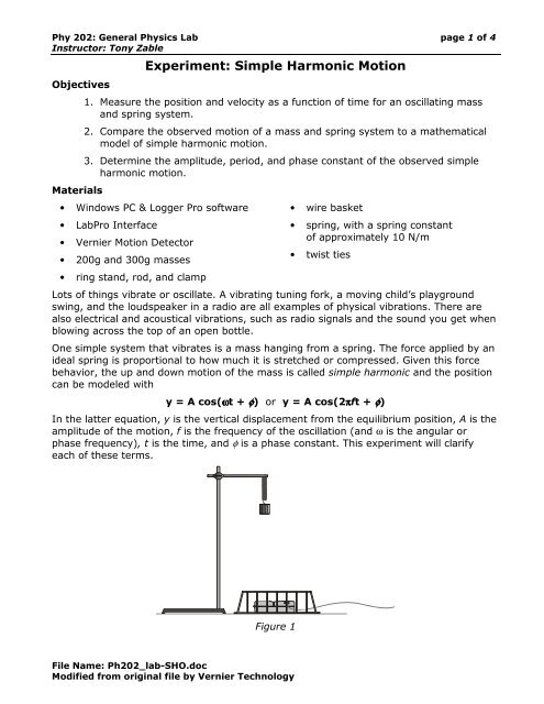
Figure 1



Preliminary Questions 

1. Attach the 200-g mass to the spring and hold the free end of the spring in your hand, 

so the mass and spring hang down with the mass at rest. Lift the mass about 10 cm 

and release. Observe the motion. Sketch a graph of position vs. time for the mass. 

2. Just below the graph of position vs. time, and using the same length time scale, sketch 

a graph of velocity vs. time for the mass. 

Procedure 

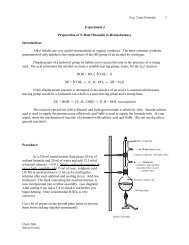
1. Attach the spring to a horizontal rod connected to the ring stand and hang the mass 

from the spring as shown in Figure 1. Securely fasten the 200g mass to the spring and 

the spring to the rod, using twist ties so the mass cannot fall. 

2. Connect the Motion Detector to Ch1 of the LabPro interface then start the LoggerPro 

software. 

3. Open the Vernier experiment file “15 Simple Harmonic Motion”. 

4. Place the Motion Detector at least 75 cm below the mass. Make sure there are no 

objects near the path between the detector and mass, such as a table edge. Place the 

wire basket over the Motion Detector to protect it. 

5. Make a preliminary run to make sure things are set up correctly. Lift the mass upward 

a few centimeters and release. The mass should oscillate along a vertical line only. 

Begin data collection. 

6. After about 10s, data collection will stop. The position graph should show a clean 

sinusoidal curve. If it has flat regions or spikes, reposition the Motion Detector and try 

again. 

7. Compare the position and velocity graphs to your sketched predictions in the 

Preliminary Questions. How are the graphs similar? How are they different? 

8. With the 200g mass hanging at rest, begin data collection. After collection stops, use 

the statistics button, , to determine the average distance from the detector. Record 

this position (yo) in the data table. 

9. Now lift the mass upward about 5 cm, release it and begin data collection. The mass 

should oscillate along a vertical line only. Examine the graphs. The pattern you are 

observing is characteristic of simple harmonic motion. 


Modified from original file by Vernier Technology



10. Using the distance graph, measure the time interval between maximum positions. 

Record the period and frequency in the data table. 

11. The amplitude, A, of simple harmonic motion is the maximum distance from the 

equilibrium position. Estimate values for the amplitude from your position graph. Enter 

the values in your data table. Click on the Examine button, , once again to turn off 

the examine mode. 

12. Repeat Steps 8 – 11 with the same 200g mass, moving with greater amplitude than 

the first run. 

13. Change the mass to 300 g and repeat Steps 7 – 11. Use an amplitude of about 5 cm. 

Keep a good run made with this 300-g mass on the screen. You will use it for several 

of the Analysis questions. 

Data Table 

Analysis 

Run Mass 

1 

2 

3 


Modified from original file by Vernier Technology 

yo 

A T 

(g) (cm) (cm) (s) (Hz) 

1. View the graphs of the last run on the screen. Compare the position vs. time and the 

velocity vs. time graphs. How are they the same? How are they different? 

2. Turn on the Examine mode by clicking the Examine button, . Move the mouse cursor 

back and forth across the graph to view the data values for the last run on the screen. 

Where is the mass when the velocity is zero? Where is the mass when the velocity is 

greatest? 

3. Does the frequency, f, appear to depend on the amplitude of the motion? Do you have 

enough data to draw a firm conclusion? 

4. Does the frequency, f, appear to depend on the mass used? Did it change much in 

your tests? 

f



5. Compare your experimental data to a sinusoidal function using the Model feature of 

LoggerPro. Try it with your 300g data. 

a. In LoggerPro, select “Analyze”→”Model” from the Data menu. 

b. Scroll down and select the “Sine” function then click on the “Define Function” 

button. Modify the sine equation to reflect the simple harmonic motion equation 

in the introduction then re-name the function to “Cosine”. Click on “OK”. 

c. Adjust the model coefficients, to reflect your measured values for yo, A, and f. 

d. Note: Since data collection did not necessarily begin when the mass was at 

maximum distance from the detector, introduction of the “phase constant” φ is 

needed (represented by the “C” parameter in LoggerPro). The optimum value 

for φ will be between 0 and 2π. Set the “C” coefficient to a value that makes the 

model come as close as possible to your data. You may also need to adjust yo, 

A, and f to improve the fit. Write the equation that best matches your data. 

7. What would happen to the plot of the model if you doubled the parameter for A? 

Sketch both the current model (from step 6) and the new model with doubled A. 

8. Adjust the model equation by doubling the parameter for A to compare to your 

prediction. How does your prediction compare to the LoggerPro model? 

9. How would the model graph change if you doubled f? Sketch both the original model 

(from step 6) and your prediction with doubled f. 

10. Adjust the LoggerPro model to reflect doubled f. How does your prediction compare to 

the LoggerPro model? 


Modified from original file by Vernier Technology

Experiment: Simple Harmonic Motion - PCC

Create successful ePaper yourself

Delete template?

Save as template?