Lecture 11 - More Fourier Transform - Electrical Engineering ...
Lecture 11 - More Fourier Transform - Electrical Engineering ...
Lecture 11 - More Fourier Transform - Electrical Engineering ...

You also want an ePaper? Increase the reach of your titles
YUMPU automatically turns print PDFs into web optimized ePapers that Google loves.
<strong>Lecture</strong> <strong>11</strong><br />
Properties of<br />
<strong>Fourier</strong> <strong>Transform</strong><br />
(Lathi 7.3-7.4)<br />
Peter Cheung<br />
Department of <strong>Electrical</strong> & Electronic <strong>Engineering</strong><br />
Imperial College London<br />
URL: www.ee.imperial.ac.uk/pcheung/teaching/ee2_signals<br />
E-mail: p.cheung@imperial.ac.uk<br />
PYKC 20-Feb-<strong>11</strong> E2.5 Signals & Linear Systems<br />
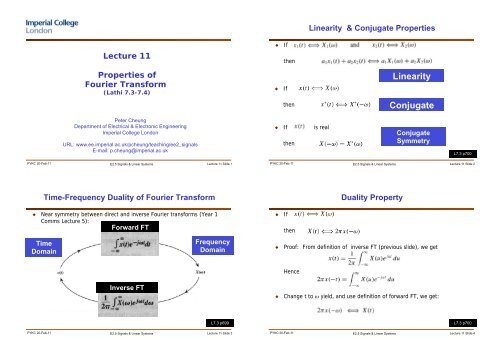
Time-Frequency Duality of <strong>Fourier</strong> <strong>Transform</strong><br />
Near symmetry between direct and inverse <strong>Fourier</strong> transforms (Year 1<br />
Comms <strong>Lecture</strong> 5):<br />
Forward FT<br />
Time<br />
Domain<br />
Inverse FT<br />
PYKC 20-Feb-<strong>11</strong> E2.5 Signals & Linear Systems<br />
<strong>Lecture</strong> <strong>11</strong> Slide 1<br />
Frequency<br />
Domain<br />
L7.3 p699<br />
<strong>Lecture</strong> <strong>11</strong> Slide 3<br />
If<br />
If<br />
then<br />
then<br />
If is real<br />
then<br />
Linearity & Conjugate Properties<br />
PYKC 20-Feb-<strong>11</strong> E2.5 Signals & Linear Systems<br />
If<br />
then<br />
Duality Property<br />
PYKC 20-Feb-<strong>11</strong> E2.5 Signals & Linear Systems<br />
Linearity<br />
Conjugate<br />
Conjugate<br />
Symmetry<br />
Proof: From definition of inverse FT (previous slide), we get<br />
Hence<br />
Change t to ω yield, and use definition of forward FT, we get:<br />
L7.3 p700<br />
<strong>Lecture</strong> <strong>11</strong> Slide 2<br />
L7.3 p700<br />
<strong>Lecture</strong> <strong>11</strong> Slide 4
Duality Property Example<br />
Consider the FT of a rectangular function:<br />
PYKC 20-Feb-<strong>11</strong> E2.5 Signals & Linear Systems<br />
If<br />
then<br />
Time-Shifting Property<br />
Consider a sinusoidal wave, time shifted:<br />
Obvious that phase shift increases with frequency (To is constant).<br />
PYKC 20-Feb-<strong>11</strong> E2.5 Signals & Linear Systems<br />
L7.3 p701<br />
<strong>Lecture</strong> <strong>11</strong> Slide 5<br />
L7.3 p705<br />
<strong>Lecture</strong> <strong>11</strong> Slide 7<br />
If<br />
then for any real constant a,<br />
Scaling Property<br />
That is, compression of a signal in time results in spectral expansion, and<br />
vice versa.<br />
PYKC 20-Feb-<strong>11</strong> E2.5 Signals & Linear Systems<br />
Time-Shifting Example<br />
Find the <strong>Fourier</strong> transform of the gate pulse x(t) given by:<br />
This pulse is rect(t/τ) dleayed by 3τ/4 sec.<br />
Use time-shifting theorem, we get<br />
PYKC 20-Feb-<strong>11</strong> E2.5 Signals & Linear Systems<br />
L7.3 p703<br />
<strong>Lecture</strong> <strong>11</strong> Slide 6<br />
L7.3 p708<br />
<strong>Lecture</strong> <strong>11</strong> Slide 8
If<br />
then<br />
Frequency-Shifting Property<br />
Multiply a signal by e jω 0 t shifts the spectrum of the signal by ω 0 .<br />
In practice, frequency shifting (or amplitude modulation) is achieved by<br />
multiplying x(t) by a sinusoid:<br />
PYKC 20-Feb-<strong>11</strong> E2.5 Signals & Linear Systems<br />
If<br />
then<br />
Convolution Properties<br />
L7.3 p709<br />
<strong>Lecture</strong> <strong>11</strong> Slide 9<br />
Let H(ω) be the <strong>Fourier</strong> transform of the unit impulse response h(t), i.e.<br />
Applying the time-convolution property to y(t)=x(t) * h(t), we get:<br />
That is: the <strong>Fourier</strong> <strong>Transform</strong> of the system impulse response is<br />
the system Frequency Response<br />
PYKC 20-Feb-<strong>11</strong> E2.5 Signals & Linear Systems<br />
L7.3 p712<br />
<strong>Lecture</strong> <strong>11</strong> Slide <strong>11</strong><br />
Frequency-Shifting Example<br />
Find and sketch the <strong>Fourier</strong> transform of the signal<br />
where xt ( ) = rectt ( / 4).<br />
PYKC 20-Feb-<strong>11</strong> E2.5 Signals & Linear Systems<br />
By definition<br />
xt ()cos10t<br />
Proof of the Time Convolution Properties<br />
The inner integral is <strong>Fourier</strong> transform of x 2 (t-τ), therefore we can use<br />
time-shift property and express this as X 2 (ω) e -jωτ .<br />
PYKC 20-Feb-<strong>11</strong> E2.5 Signals & Linear Systems<br />
L7.3 p710<br />
<strong>Lecture</strong> <strong>11</strong> Slide 10<br />
L7.3 p712<br />
<strong>Lecture</strong> <strong>11</strong> Slide 12
Frequency Convolution Example<br />
Find the spectrum of xt ()cos10t<br />
where x( t) = rect( t / 4). using<br />
convolution property.<br />
x<br />
PYKC 20-Feb-<strong>11</strong> E2.5 Signals & Linear Systems<br />
1/2<br />
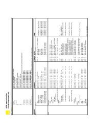
Summary of <strong>Fourier</strong> <strong>Transform</strong> Operations (1)<br />
PYKC 20-Feb-<strong>11</strong> E2.5 Signals & Linear Systems<br />
*<br />
1/2<br />
<strong>Lecture</strong> <strong>11</strong> Slide 13<br />
L7.3 p715<br />
<strong>Lecture</strong> <strong>11</strong> Slide 15<br />
If<br />
then<br />
and<br />
Time Differentiation Property<br />
Compare with Lec 6/17, Time-differentiation property of Laplace<br />
transform:<br />
PYKC 20-Feb-<strong>11</strong> E2.5 Signals & Linear Systems<br />
Summary of <strong>Fourier</strong> <strong>Transform</strong> Operations (2)<br />
PYKC 20-Feb-<strong>11</strong> E2.5 Signals & Linear Systems<br />
L7.3 p714<br />
<strong>Lecture</strong> <strong>11</strong> Slide 14<br />
L7.3 p715<br />
<strong>Lecture</strong> <strong>11</strong> Slide 16