Eisenstein series and approximations to pi - Mathematics

EISENSTEIN SERIES AND APPROXIMATIONS TO π
Bruce C. Berndt and Heng Huat Chan
Dedicated to K. Venkatachaliengar
1. Introduction
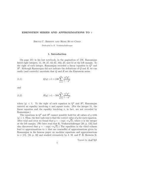
On page 211 in his lost notebook, in the pagination of [19], Ramanujan
listed eight integers, 11, 19, 27, 43, 67, 163, 35, and 51 at the left margin. To
the right of each integer, Ramanujan recorded a linear equation in Q 3 and
R 2 . Although Ramanujan did not indicate the definitions of Q and R, we can
easily (and correctly) ascertain that Q and R are the Eisenstein series
(1.1)
and
(1.2)
Q(q) :=1 + 240
R(q) :=1 − 504
∞
n=1
∞
n=1
n 3 q n
1 − q n
n5qn ,
1 − qn where |q| < 1. To the right of each equation in Q 3 and R 2 , Ramanujan
entered an equality involving π and square roots. (For the integer 51, the
linear equation and the equality involving π, in fact, are not recorded by
Ramanujan.)
The equations in Q 3 and R 2 cannot possibly hold for all values of q with
|q| < 1. Thus, the first task was to find the correct value of q for each equation.
After trial and error we found that q = − exp(−π √ n), where n is the integer
at the left margin. (We later read that K. Venkatachaliengar [20, p. 135] had
also discovered that q = − exp(−π √ n).) The equalities in the third column
lead to approximations to π that are remindful of approximations given by
Ramanujan in his famous paper on modular equations and approximations
to π [15], [18, p. 33] and studied extensively by J. M. and P. B. Borwein [6,
1
Typeset by AMS-TEX

2 BRUCE C. BERNDT AND HENG HUAT CHAN
Chap. 5]. As will be seen, this page in the lost notebook is closely connected
with theorems connected with the modular j-invariant stated by Ramanujan
on the last two pages of his third notebook [10] and proved by the authors
[4], [3, pp. 309–322].
In Section 2, we prove a general theorem from which the linear equations
in Q 3 and R 2 in the second column follow as corollaries. In Sections 3 and 4,
we offer two methods for proving the equalities in the third column and show
how they lead to approximations to π. Ramanujan’s equations for π lead in
Section 4 to certain numbers tn (defined by (4.28)). The numbers tn guide us
in Section 5 to a proof of a general series formula for 1/π, which is equivalent
to a formula found by D. V. and G. V. Chudnovsky [13] and the Borweins [9].
The first series representations for 1/π of this type were found by Ramanujan
[15], [18, pp. 23–39] but first proved by the Borweins [8]. The work of the
Borweins [6], [7], [8] and Chudnovskys [13] significantly extends Ramanujan’s
work. One of Ramanujan’s series for 1/π yields 8 digits of π per term, while
one of the Borweins [7] gives 50 digits of π per term. Our simpler method
enables us in Section 5 to determine a series for 1/π which yields about 73 or
74 digits of π per term.
2. Eisenstein Series and the Modular j–invariant
Recall the definition of the modular j–invariant j(τ),
(2.1) j(τ) = 1728
Q 3 (q)
In particular, if n is a positive integer,
√
3 + −n
(2.2) j
2
where, for brevity, we set
Q 3 (q) − R 2 (q) , q = e2πiτ , Im τ > 0.
= 1728 Q3n Q3 n − R2 ,
n
(2.3) Qn := Q(−e −π√ n ) and Rn := R(−e −π√ n ).
In his third notebook, at the top of page 392 in the pagination of [17], Ramanujan
defined a certain function Jn of singular moduli, which, as the authors [4]
easily showed, has the representation
(2.4) Jn = − 1
√
3 3 + −n
j
.
32 2
Hence, from (2.2) and (2.4),
(2.5) (−32Jn) 3 = 1728 Q3 n
Q 3 n − R 2 n
.
After a simple manipulation of (2.5), we deduce the following theorem.

Theorem 2.1. For each positive integer n,
8
(2.6)
3 Jn
APPROXIMATIONS TO π 3
3
+ 1
Q 3
8
n −
3 Jn
3 R 2 n = 0,
where Jn is defined by (2.4), and Qn and Rn are defined by (2.3).
Examples 2.2 ([19, p. 211]). We have
and
539Q 3 11 − 512R 2 11 =0,
(8 3 + 1)Q 3 19 − 8 3 R 2 19 =0,
(40 3 + 9)Q 3 27 − 40 3 R 2 27 =0,
(80 3 + 1)Q 3 43 − 80 3 R 2 43 =0,
(440 3 + 1)Q 3 67 − 440 3 R 2 67 =0,
(53360 3 + 1)Q 3 163 − 53360 3 R 2 163 =0,
((60 + 28 √ 5) 3 + 27)Q 3 35 − (60 + 28 √ 5) 3 R 2 35 =0,
((4(4 + √ 17) 2/3 (5 + √ 17)) 3 + 1)Q 3 51 − (4(4 + √ 17) 2/3 (5 + √ 17)) 3 R 2 51 = 0.
Proof. In [4], [3, pp. 310, 311], we showed that
(2.7)
⎧
J11 =1,
⎪⎨
J67 =165,
⎪⎩ J35 = √
1 +
5
√ 4 5
,
2
J27 =5 · 3 1/3 ,
J19 =3,
J43 =30,
J163 =20, 010,
J51 =3(4 + √ 17) 2/3
5 + √
17
.
2
Using (2.7) in (2.6), we readily deduce all eight equations in Qn and Rn.
3. Eisenstein Series and Equations in π - First Method
Define, after Ramanujan,
(3.1) P (q) := 1 − 24
∞
n=1
nqn , |q| < 1,
1 − qn

4 BRUCE C. BERNDT AND HENG HUAT CHAN
and put
(3.2) Pn := P (−e −π√ n ).
Next, set
(3.3) bn = {n(1728 − jn)} 1/2
and
(3.4) an = 1
6 bn
1 − Qn
Pn −
Rn
6
π √
.
n
The numbers an and bn arise in series representations for 1/π proved by the
Chudnovskys [13] and the Borweins [8], namely,
(3.5)
1 1
= √
π −jn
∞
k=0
(6k)!
(3k)!(k!) 3
an + kbn
jk ,
n
where (c)0 = 1, (c)k = c(c + 1) · · · (c + k − 1), for k ≥ 1, and
√
3 + −n
jn = j
.
2
These authors have calculated an and bn for several values of n, but we are
uncertain if these calculations are theoretically grounded. We show how (3.3)
and (3.4) lead to a formula from which Ramanujan’s equalities in the third
column on page 211 follow.
From (2.6), we easily see that
(3.6)
Qn
Rn
and from (3.4), we find that
(3.7)
Qn
Rn
= 1
8
√
Qn
3 Jn
8
3 Jn
3 + 1
3
−1/2
6
π − √
nPn = 6 √ n an
−
bn
√ n.
The substitution of (3.6) into (3.7) leads to the following theorem.
,

APPROXIMATIONS TO π 5
Theorem 3.1. If Pn, bn, an, and Jn are defined by (3.2)–(3.4) and (2.4),
respectively, then
(3.8)
1
√ Qn
√nPn
− 6
=
π
√
n 1 − 6 an
bn
8
Examples 3.2 ([19, p. 211]). We have
3 Jn
8
3 Jn
3 + 1
1 √11P11 √ −
Q11
6
=
π
√ 2,
1 √19P19 √ −
Q19
6
=
π
√ 6,
1 √27P27 √ −
Q27
6
6
=3
π 5 ,
1 √43P43 √ −
Q43
6
3
=6
π 5 ,
1 √67P67 √ −
Q67
6
6
=19
π 55 ,
1 √163P163 √ −
Q163
6
3
=362
π 3335 ,
1 √35P35 √ −
Q35
6
=(2 +
π
√
2
5) √ ,
5
1 √51P51 √ −
Q51
6
=.
π
3
1/2
Ramanujan’s formulation of the first example of Examples 3.2 is apparently
given by
√ 6
11 − + · · ·
π
3 1
1 − 240 · · ·
= √ 2.
e π√ 11
(The denominator with 1 3 in the numerator is unreadable.) Further equalities
are even briefer, with √ Qn replaced by √ ·. Note that Pn is replaced by
“1 + · · · ” in Ramanujan’s examples. Also observe that Ramanujan did not
record the right side when n = 51. Because it is unwieldy, we also have not
.

6 BRUCE C. BERNDT AND HENG HUAT CHAN
recorded it. However, readers can readily complete the equality, since J51 is
given in (2.7) and a51 and b51 are given in the next table.
Proof. The first six values of an and bn were calculated by the Borweins [8,
pp. 371, 372]. The values for n = 35 and 51 were calculated by the present
authors. We record all 8 pairs of values for an and bn in the following table.
n an bn
11 60 616
19 300 4104
27 1116 18216
43 9468 195048
67 122124 3140424
163 163096908 6541681608
35 1740 + 768 √ 5 32200 + 14336 √ 5
51 11820 + 2880 √ 17 265608 + 64512 √ 17
If we substitute these values of an and bn in Theorem 3.1, we obtain, after
some calculation and simplification, Ramanujan’s equalities.
Theorem 3.1 and the last set of examples yield approximations to π. Let
rn denote the algebraic expression on the right side in (3.8). If we use the
expansions
Pn = 1 + 24e −π√ n − · · · and Qn = 1 − 120e −π√ n + · · · ,
we easily find that
π =
6
√
n − rn
1 − 24√n + 120rn
√
n − rn
We thus have proved the following theorem.
Theorem 3.3. We have
π ≈
with the error approximately equal to
6
√ =: An,
n − rn
√
n + 5rn
144
( √ n − rn) 2 e−π√ n
,
e −π√
n
+ · · · .

APPROXIMATIONS TO π 7
where rn is the algebraic expression on the right side in (3.8).
See Ramanujan’s paper [15], [18, p. 33] for other approximations to π of
this sort.
In the table below, we record the decimal expansion of each approximation
An and the number Nn of digits of π agreeing with the approximation.
n An Nn
11 3.1538 . . . 1
19 3.1423 . . . 2
27 3.1416621 . . . 3
43 3.141593 . . . 5
67 3.14159266 . . . 7
163 3.14159265358980 . . . 12
35 3.141601 . . . 3
51 3.14159289 . . . 6
4. Eisenstein Series and Equations in π - Second Method
Set P := P(q) := P (−q), Q := Q(q) := Q(−q), R := R(q) := R(−q),
∆ := ∆(q) := Q3 (q)−R2 (q), and J := J(q) := 1728/j
3+τ
2πiτ
2 , where q = e .
Set
(4.1) z 4 := Q =
1/3 ∆
,
J
by (2.1). Then, by (4.1) and the definition of ∆,
(4.2) R = Q 3 − ∆ =
∆√
6
1 − J = z
J
√ 1 − J.
Recall the differential equations [16], [17, p. 142]
(4.3)
q dP
dq = P 2 (q) − Q(q)
, q
12
dQ P (q)Q(q) − R(q)
= , q
dq 3
dR
dq = P (q)R(q) − Q2 (q)
,
2
which yield the associated differential equations
(4.4)
q dP
dq = P2 (q) − Q(q)
, q
12
dQ P(q)Q(q) − R(q)
= , q
dq 3
dR
dq = P(q)R(q) − Q2 (q)
.
2

8 BRUCE C. BERNDT AND HENG HUAT CHAN
Now, by rearranging the second equation in (4.4), with the help of (4.1)
and (4.2), we find that
(4.5) P(q) = R(q) 12q dz
+
Q(q) z dq .
From the chain rule and (4.5), it follows that, for any positive integer n,
P(q n ) = R(qn )
Q(qn 12q
+
) nz(qn )
Subtracting (4.5) from the last equality and setting
we find that
(4.6)
nP(q n ) − P(q) =n R(qn )
Q(qn R(q)
−
) Q(q)
m := z(q)
z(q n ) ,
q
+ 12
z(qn )
=n R(qn )
Q(qn R(q) q dm
− − 12
) Q(q) m dq .
dz(qn )
.
dq
dz(q n )
dq
q dz(q)
− 12
z(q) dq
Our next aim is to replace dm
dm
in (4.6) by
dq dJ (J(q), J(qn )). From (2.1),
the definition of J, (4.4), (4.1), and (4.2), upon differentiation, we find that
(4.7)
q dJ
dq =(3Q2 Q ′ − 2RR ′ )Q3 − 3Q2Q ′ (Q3 − R2 )
Q6 = {Q2 (PQ − R) − R(PR − Q 2 )}Q 3 − Q 2 (PQ − R)(Q 3 − R 2 )
Q 6
= RQ3 − R 3
Q 4
which implies that
= R∆
Q 4 = z6√ 1 − J J
Q = z2 J √ 1 − J,
(4.8) z 2 1
(q) =
J(q) dJ(q)
q
1 − J(q) dq .
Replacing q by q n in (4.8) and simplifying, we deduce that
(4.9) z 2 (q n ) =
1
nJ(qn ) 1 − J(qn ) q dJ(qn )
.
dq

Using (4.8) and (4.9), we conclude that
(4.10) m 2 = n J(qn ) 1 − J(q n )
J(q) 1 − J(q)
APPROXIMATIONS TO π 9
dJ(q)
dJ(qn ) .
It is well known that there is a relation (known as the class equation) between
j(τ) and j(nτ) for any integer n [14, p. 231, Theorem 11.18(i)]. With
the definition of J given at the beginning of this section, the class equation
translates to a relation between J(q) and J(q n ). It follows that,
(4.11)
dJ(q)
dJ(q n ) = F (J(q), J(qn )),
for some rational function F (x, y). Thus, by (4.10) and (4.11), we may differentiate
m with respect to J, and so, by (4.7) and the definition of m(q),
2 q dm
m(q) dq = 2z(q)z(qn )
Using this in (4.6), we deduce that
(4.12)
nP(q n ) − P(q)
z(q)z(q n )
q
z2 (q)
dm
dq
= 2z 2 (q n )m(q) dm dJ
q
dJ dq = z2 (q n )J √ 1 − J dm2 (q)
dJ .
= n R(qn )
Q(qn R(q)
−
) Q(q) − 6z2 (q n )J(q) 1 − J(q) dm2
dJ .
If we put q = e −π/√ n , n > 0, (4.12) takes the shape
nP(e −π√n −π/
) − P(e √ n R(e
) =n −π√n )
Q(e−π√ −
n ) R(e−π/√ n )
Q(e−π/√n )
− 6z 2 (e −π√n −π/
)J(e √
n
) 1 − J(e−π/√n )
× dm2
J(e
dJ
−π√n −π/
), J(e √
n
(4.13)
) .
It is well known that [12, p. 84]
(4.14) J(e −π/√ n ) = J(e −π √ n ).
Furthermore, if
(4.15) ϕ(q) =
∞
n=−∞
q n2
and ψ(q) =
∞
q n(n+1)/2 , |q| < 1,
n=0

10 BRUCE C. BERNDT AND HENG HUAT CHAN
then [2, p. 127, Entries 13(iii), (iv)],
(4.16)
and
(4.17)
Q(q) = z 4 2(1 + 14x2 + x 2 2),
R(q) = z 6 2(1 + x2)(1 − 34x2 + x 2 2),
where [2, p. 122–123, Entries 10(i), 11(iii)]
(4.18) z2 := ϕ 2 (q) and x2 := 16q ψ4 (q 2 )
ϕ 4 (q) .
Replacing q by −q in (4.16) and (4.17), and using (4.18), we find that
(4.19)
and
(4.20)
Q(q) = ϕ 8 (−q) − 224qϕ 4 (−q)ψ 4 (q 2 ) + 16 2 q 2 ψ 8 (q 2 )
R(q) = (ϕ 4 (−q) − 16qψ 4 (q 2 ))
× (ϕ 8 (−q) + 544qϕ 4 (−q)ψ 4 (q 2 ) + 16 2 q 2 ψ 8 (q 2 )).
Using the transformation formula [2, p. 43, Entry 27(ii)],
in (4.19) and (4.20), we deduce that
(4.21)
and
(4.22)
ϕ(e −π/t ) = 2e −πt/4√ tψ(e −2πt )
R(e −π/√ n ) = −n 3 R(e −π √ n )
Q(e −π/√ n ) = n 2 Q(e −π √ n ).
Using (4.14), (4.21), and (4.22), we may rewrite (4.13) as
nP(e −π√n −π/
) − P(e √ n
)
= 2n R(e−π√ n )
Q(e−π√ − 6z
n ) 2 (e −π√
n dm
)Jn 1 − J1/n 2
dJ (Jn, Jn) ,
= 2n
dm
1 − Jn − 6Jn 1 − J1/n 2
dJ (Jn,
(4.23)
Jn)
z 2 (e −π√ n ),

where
APPROXIMATIONS TO π 11
(4.24) Jk = J(e −π√ k ), k > 0.
This gives the first relation between P(e −π√ n ) and P(e −π/ √ n ).
Recall the definitions of Ramanujan’s function f(−q) and the Dedekind
eta-function η(τ), namely,
f(−q) :=
∞
(1 − q k ) =: e −2πiτ/24 η(τ), q = e 2πiτ , Im τ > 0.
k=1
The function f satisfies the well-known transformation formula [2, p. 43]
(4.25) n 1/4 e −π√ n/24 f(e −π √ n ) = e −π/(24 √ n) f(e −π/ √ n ), n > 0.
Logarithmically differentiating (4.25) with respect to n, multiplying both sides
by 48n 3/2 /π, rearranging terms, and employing the definition of P (q) given
in (3.1), we find that
(4.26)
12 √ n
π = nP(e−π√ n ) + P(e −π/ √ n ).
This gives a second relation between P(e −π√ n ) and P(e −π/ √ n ).
Now adding (4.23) and (4.26) and dividing by 2, we arrive at
nP(e −π√n 6
) = √ n
π +
n
dm
1 − Jn − 3Jn 1 − J1/n 2
dJ (Jn,
Jn) z 2 (e −π√n ),
or, by (4.1),
1
√ Pn −
Qn
6
√ =
nπ
1 − J1/n
1 − Jn 1 − 3Jn
n √ dm
1 − Jn
2
dJ (Jn,
Jn) ,
where Qn is defined by (2.3), and Pn is defined by (3.2). (Be careful; Jn = Jn,
where Jn is defined by (2.4).)
We record the last result in the following theorem, which should be compared
with Theorem 3.1.
Theorem 4.1. If Pn, Qn, and Jn
respectively, then
are defined by (3.2), (2.3), and (4.24),
(4.27)
1
√ Pn −
Qn
6
√ =
nπ
1 − Jntn,

12 BRUCE C. BERNDT AND HENG HUAT CHAN
where
1 − J1/n
(4.28) tn := 1 − 3Jn
n √ 1 − Jn
Observe that, by (4.1), (4.2), and Theorem 2.1,
(4.29)
1 − Jn =
8
3Jn
8
3Jn 3 dm2 dJ (Jn,
Jn) .
3 + 1
1/2
Hence, the values of √ 1 − Jn for those n given on page 211 of the Lost Notebook
follow immediately from (2.7). In order to rederive Examples 3.2, it
suffices to compute tn.
Theorem 4.2. If n > 1 is an odd positive integer, then tn lies in the ring
class field of Z[ √ −n].
Proof. By differentiating (4.10) with respect to J(q), we conclude that
(4.30)
dm2 dJ(q) =
1 − J(qn )
G(J(q), J(q
1 − J(q) n )),
for some rational function G(J(q), J(q n )). Using (4.28) and (4.30), we find
that tn can be expressed in terms of Jn. Since Jn is in the ring class field
of Z[ √ −n] when n > 1 is odd and squarefree [14, p. 220, Theorem 11.1], we
complete our proof.
An equivalent form of Theorem 4.2 is first mentioned without proof and
conditions on n by the Chudnovskys on page 391 of [13].
Theorem 4.2 allows us to devise an empirical process for deriving tn whenever
the class group of Q( √ −n) is of the type Zr 2, r ∈ N, where r = 0 refers to
imaginary quadratic fields with class number 1. By (3.6), (4.27), and (4.29),
we find that
(4.31) tn = Qn
Pn − 6
√ .
nπ
Rn
When r = 0, we numerically compute the right hand side of (4.31) using the
definitions of Pn, Qn, and Rn, and then using the command “minpoly(tn,1)”
on the computer algebra system MAPLE V, we derive the values of tn for
n = 3, 7, 11, 19, 27, 43, 67 and 163. We summarize our findings in the following
table.
.

APPROXIMATIONS TO π 13
n tn
3 0
5
7
21
32
11
77
32
19
57
160
27
253
640
43
903
67
163
33440
43617
77265280
90856689
When r = 1, we are in a situation where tn satisfies a polynomial of degree
2. We use the command “minpoly(tn,2)” and derive the resulting polynomial
satisfied by tn. Using this method, we could, in particular, determine tn for
n = 35 and 51, namely,
t35 = 1504 + 576√ 5
4123
and t51 = 144
329 + 400√ 17
5593 .
Using the values of tn given in the tables above and Theorem 4.1, we rederive
Examples 3.2.
So far, our method is still similar to that of the Borweins and Chudnovskys.
Of course, we could continue to use “minpoly” and derive minimal polynomials
satisfied by tn for r = 2, 3, and 4. However, this means that we have to solve
polynomials of degress 4, 8, and 16, respectively, which is cumbersome when
the degree of the polynomial exceeds 4. We now describe a new process for
deriving tn, for r > 1. We illustrate our method using n = 21.
When n = 21, we numerically compute t21 and t 7/3 and use “minpoly” to
deduce that
and
Solving for t21 yields
t21 + t7/3 = 30493 3820 √
+ 7
34279 34279
√
3(t21 − t7/3) = 28800 1935 √
+ 7.
34279 34279
t21 = 30493 645 √ 4800 √ 1910 √
+ 21 + 3 − 7.
68558 68558 34279 34279

14 BRUCE C. BERNDT AND HENG HUAT CHAN
The largest n for which tn can be computed using this new empirical
method is n = 3315, namely,
t3315 := 1095255033002752301233099478037584
2050242335692983321671746996556833
+ 1006588064225996719872149534306400 √ √
17 5
34854119706780716468419698941466161
+ 692779168175128551453280427070000 √
17
34854119706780716468419698941466161
− 136434536163779492503565618457696 √
5
2050242335692983321671746996556833
+ 400179322879781860521299209248000 √
13
26653150364008783181732710955238829
+ 1077564413015882021519209726762688 √ √ √
13 17 5
453103556188149314089456086239060093
+ 120226784218523863048087030809600 √ √
17 13
64729079455449902012779440891294299
+ 239369594240980944219359445009600 √ √
13 5.
26653150364008783181732710955238829
This value is deduced from determining the quadratic numbers
t3315 + t 1105/3 + t 663/5 + t 221/15,
√ 221(t3315 − t 1105/3 + t 663/5 − t 221/15),
√ 13(t3315 + t 1105/3 − t 663/5 − t 221/15),
and √ 5(t3315 − t 1105/3 − t 663/5 + t 221/15)
in Q( √ 85). We show in the next section that knowledge of t3315 and J3315
leads to a new series for 1/π which converges at a rate of 73/74 decimal places

APPROXIMATIONS TO π 15
per term. This series appears to be the fastest known convergent series for
1/π which involves quadratic radicals. The previous fastest convergent series,
giving 50 decimal places per term, was obtained by the Borweins [8]. Their
series involves quartic radicals which arise from the field Q( √ −1555), which
has class number 4.
5. tn, Jn and the Ramanujan–Borweins–Chudnovskys series for 1/π
Let ϕ(q) and ψ(q) be given as in (4.15), and recall the definition of the
hypergeometric function 2F1,
2F1(a, b; c; u) :=
∞ (a)k(b)k
k=0
(c)k
uk , |u| < 1.
k!
In [20], using Ramanujan’s differential equations (4.3) and the relations
Q(q 2 ) = z 4 2(1 − x2 + x 2 2) and R(q 2 ) = z 6 2(1 + x2)(1 − 2x2)(1 − x2/2),
where z2 and x2 are given by (4.18), Venkatachaliengar proved the inversion
formula
z2 = 2F1( 1 1
2 , 2 ; 1; x2).
His method can be applied whenever we have relations of the form
Q(q) = z 4 F (x) and R(q) = z 6 G(x),
for some function z and x. The relations (4.1) and (4.2) indicate that we are
in such a situation with z := Q and x := J. Invoking Venkatachaliengar’s
method (see [11], [10] for examples of such calculations), we readily deduce
that
(5.1) z = 2F1( 1 5
12 , 12 ; 1; J).
We are now ready to give a proof of an equivalent form of the general series
for 1/π given by (3.5). As far as we know, a proof of this series has never
been written down in the literature. First, by Clausen’s formula [1, p. 116],
we find that
(5.2) z 2 = 2F1( 1 5
12 ,
where
3F2(a, b, c; d, e; u) =
12 ; 1; J) 2
= 3F2( 1
6
∞ (a)k(b)k(c)k
k=0
(d)k(e)k
5 1 , 6 , 2 ; 1, 1; J),
uk , |u| < 1.
k!

16 BRUCE C. BERNDT AND HENG HUAT CHAN
This implies, by (5.1), that
(5.3) 2z dz
dJ =
where
Ak :=
By (4.5) and (4.7), we deduce that
(5.4) 2z dz 1
=
dJ 6J
∞
AkkJ k−1 ,
k=1
1
6 k
5
6 k
(k!) 3
1
2
k
P
√ − z
1 − J 2
.
Substituting (5.4) into (5.3) and using (5.2), we deduce that
(5.5)
P
√ 1 − J =
∞
Ak(6k + 1)J k .
k=0
Next, set q = e −π√ n and deduce from (5.5) that
(5.6)
Pn
√ =
1 − Jn
∞
Ak(6k + 1)J k n.
k=0
On the other hand, by Theorem 4.1 and (4.1),
(5.7) Pn = 6
π √ n + z2
n 1 − Jntn.
Using (5.7), (5.2) (with z replaced by zn and J replaced by Jn) and (5.6), we
conclude that
6 1
(5.8) √ √
n 1 − Jn π =
∞
1 5 1
6 k 6 k 2 k
(k!) 3 J k n(6k + 1 − tn).
k=0
It can be shown that (5.8) is equivalent to the Ramanujan–Borweins–Chudnovskys
series. The series (5.8) enables us to write down for each n, a series for
1/π if we know the values of tn and Jn.
We have already determined the value of t3315 in Section 4. It suffices
to compute J3315 in order to write down a series for 1/π associated with
n = 3315. We first quote the identity [4], [5]
√
3 + −3n
(5.9) j
2
= −27 (λ2n − 1)(9λ2 n − 1) 3
λ2 ,
n
.

where
APPROXIMATIONS TO π 17
λn = eπ√ n/2
3 √ 3
f 6 (e −π√ n/3 )
f 6 (e −π√ 3n ) ,
where f(−q) is defined prior to (4.25). Since [5]
λ 2 1105 =
√ 5 + 1
2
24
(4 + √ 17) 6
15 + √ 6 221
(8 +
2
√ 65) 6 ,
the value of J3315 follows immediately from (5.9). The values J3315 and t3315,
when substituted into (5.8), yield the series which we mentioned at the end
of Section 4.
Acknowledgement. We are grateful to Seung Hwan Son for helping us find the
correct value of q for the linear equations in Q 3 and R 2 . The first author is
grateful to the National University of Singapore for financially supporting his
visit there when this research was conducted.
References
1. G. E. Andrews, R. A. Askey, and R. Roy, Special Functions, Cambridge University
Press, Cambridge, 1999.
2. B. C. Berndt, Ramanujan’s Notebooks, Part III, Springer–Verlag, New York, 1991.
3. B. C. Berndt, Ramanujan’s Notebooks, Part V, Springer–Verlag, New York, 1998.
4. B. C. Berndt and H. H. Chan, Ramanujan and the modular j–invariant, Canad.
Math. Bull. 42 (1999), 427–440.
5. B. C. Berndt, H. H. Chan, S.–Y. Kang, and L.–C. Zhang, A certain quotient of
eta-functions found in Ramanujan’s lost notebook,, Pacific J. Math. (to appear).
6. J. M. Borwein and P. M. Borwein, Pi and the AGM, Wiley, New York, 1987.
7. J. M. Borwein and P. B. Borwein, Ramanujan’s rational and algebraic series for 1/π,
Indian J. Math. 51 (1987), 147–160.
8. J. M. Borwein and P. M. Borwein, More Ramanujan-type series for 1/π, Ramanujan
Revisited (G. E. Andrews, R. A. Askey, B. C. Berndt, K. G. Ramanathan, and R. A.
Rankin, eds.), Academic Press, Boston, 1988, pp. 359–374.
9. J. M. Borwein and P. B. Borwein, Some observations on computer aided analysis,
Notices Amer. Math. Soc. 39 (1992), 825–829.
10. H. H. Chan, On Ramanujan’s cubic transformation formula for 2F1(1/3, 2/3; 1; z),
Math. Proc. Cambridge Philos. Soc. 124 (1998), 193–204.
11. H. H. Chan and Y. L. Ong, On Eisenstein series and∞
m,n=−∞ qm2 +mn+2n 2
, Proc.
Amer. Math. Soc. 127 (1999), 1735–1744.
12. K. Chandrasekharan, Elliptic Functions, Springer–Verlag, Berlin, 1985.
13. D. V. Chudnovsky and G. V. Chudnovsky, Approximation and complex multiplication
according to Ramanujan, Ramanujan Revisited (G. E. Andrews, R. A. Askey, B. C.
Berndt, K. G. Ramanathan, and R. A. Rankin, eds.), Academic Press, Boston, 1988,
pp. 375–472.
14. D. A. Cox, Primes of the Form x2 + ny2 , Wiley, New York, 1989.

18 BRUCE C. BERNDT AND HENG HUAT CHAN
15. S. Ramanujan, Modular equations and approximations to π, Quart. J. Math. 45
(1914), 350–372.
16. S. Ramanujan, On certain arithmetical functions, Trans. Cambridge Philos. Soc. 22
(1916), 159–184.
17. S. Ramanujan, Collected Papers, Cambridge University Press, Cambridge, 1927;
reprinted by Chelsea, New York, 1962; reprinted by the American Mathematical
Society, Providence, 2000.
18. S. Ramanujan, Notebooks (2 volumes), Tata Institute of Fundamental Research, Bombay,
1957.
19. S. Ramanujan, The Lost Notebook and Other Unpublished Papers, Narosa, New Delhi,
1988.
20. K. Venkatachaliengar, Development of Elliptic Functions According to Ramanujan,
Tech. Rep. 2, Madurai Kamaraj University, Madurai, 1988.
E-mail address: berndt@math.uiuc.edu
E-mail address: chanhh@math.nus.edu.sg