User manual for Iode - Department of Mathematics

User manual for
Iode
(graphical user interface)
Peter Brinkmann and Richard Laugesen
Department of Mathematics
University of Illinois, Urbana–Champaign, U.S.A.
March 5, 2010

2
Copyright (c) 2003, The Triode (iode@math.uiuc.edu)
Permission is granted to copy, distribute and/or modify this document under
the terms of the GNU Free Documentation License, Version 1.2 or any later
version published by the Free Software Foundation; with no Invariant Sections,
no Front-Cover Texts, and no Back-Cover Texts. A copy of the license
is available at http://www.fsf.org/copyleft/fdl.html.

Contents
1 Direction fields 11
2 Phase planes 15
3 Second order linear ODEs 19
4 Fourier series 21
5 Partial differential equations 25
A Installing Iode 29
B Running Iode 31
C Reference materials 33
D Structure of Iode 37
3

4 CONTENTS

Overview
Iode (rhymes with diode) is a software package that enables you to explore
direction fields, phase planes, second order linear ODEs, Fourier series and
heat and wave equations. The name Iode is supposed to be reminiscent of
“Illinois” and “ODE”.
Iode runs under either Matlab or Octave (their programming languages
are mostly compatible). For instructions on downloading, installing and
running all the needed software, see Appendix A. If your computer already
has Matlab or Octave installed, then all you need get is Iode. Experienced
users can proceed directly to www.math.uiuc.edu/iode/ to download it.
The graphical user interface for Iode is supported only under Matlab,
version 6.0 or later, and is described in this manual. The text-based user
interface runs under earlier versions of Matlab and also under Octave, and
is described in another manual. The graphical user interface offers certain
features and plotting options that are unavailable in the text-based interface.
A good way to learn Iode is simply to explore it. Choose various options
and see what happens. Also, the built-in help features in Matlab and Octave
are your friends. For example, typing help euler at the prompt will give
information on the module euler.m.
Please let us know if you encounter problems with Iode, or if you want
to suggest new features: email us at iode@math.uiuc.edu.
From a programming perspective, the main point of Iode is that it is modular
and has well-defined interfaces. This has several useful consequences.
For example, it is easy for the user to customize Iode, or to create and plug in
new modules. Simple modules of this sort can be created even by users without
much programming experience. In fact, Iode was born out of frustration
with other educational packages that conceal their inner workings from the
user.
The mathematical modules (such as df.m or euler.m) can be used in
5

6 CONTENTS
Matlab and Octave without the graphical user interface, and much of the
code is easily extensible. Users are encouraged, and in some of our classes
expected, to look at the code and modify it, take it apart, put it back together,
and so on. For example, Appendix D discusses how to create your own solver
module for numerically solving ODEs. On the other hand, Iode’s graphical
user interface gives you access to most of the mathematical power of the
underlying modules, without requiring you to program at all. This manual
concentrates mostly on explaining the graphical user interface.

General features
Launching the Iode graphical user interface (see instructions in Appendix B)
gets you to the main menu:
Direction fields
Phase planes
Second order linear ODEs
Fourier series
Partial differential equations
Exit
You can launch these modules independently, and can even launch multiple
copies of each module. Before looking at these modules in detail, we
explain some features that are common to all (or most) of them.
Every window contains one or two graphs, as well as a number of controls
for affecting those graphs. And across the top of each window is a menu bar
whose entries include File, Equation (or Function), and Options.
The File menu deals with the outside world, such as files and printers.
The Equation menu deals with the mathematical content of your window,
i.e., it controls what you’re looking at. The Options menu contains the
display options, i.e., it controls how you’re looking at the contents of your
window.
Next we describe those menu items that are shared by all modules. Then
we’ll come to more detailed chapters on each module in turn.
File menu
The File menu is the same for all components of Iode.
• Open a file containing previously-saved settings for the window.
7

8 CONTENTS
• Save a file containing the current settings of the window. (The file
name should be entered in the Selection window of the dialog box,
and should have extension .mat.) The point is that you can Save your
work and then Open it again later.
• Print. By default, this will print the entire current window. If you
just want to print the graphs and not the rest of the window, choose
Print and then click on the Options button. In the resulting dialog,
check the box labeled “Suppress printing of user interface controls”,
then click on OK.
If you choose to print to a file instead of to a printer then you can
write your plot as a .ps file, which can then be opened and viewed
with Ghostview. (For example, on a Unix system you would get to a
Unix prompt, outside of Matlab, and type ghostview my plot.eps.)
• Quit will exit from the module.
Equation (or Function) menu
The Equation (or Function) menus have just one entry in common.
• Relabel variables: this item allows you to choose new names for the
independent as well as dependent variables.
Options menu
The Options menus have one entry in common.
• Enter caption: this item lets you put a caption at the very bottom
of the window, and is useful for adding annotations (e.g., your name,
or the number of a homework assignment).
Miscellaneous features
[Error handling.] In any of Iode’s dialog boxes, if Iode cannot make sense
of the information you provide then it will produce an error message and
simply keep the previous values. For example, a common mistake is to forget

CONTENTS 9
to type “*” to indicate multiplication. If you are asked to enter a function
and type 2xy as 2xy, then Iode will report an error and will continue using
the previous function. (The correct input for 2xy is 2*x*y.)
[Interrupting.] Matlab lacks proper mechanisms for interrupting lengthy
computations, so that there are only two solutions if a computation takes a
long time to finish: Either you wait until the computation is done, or you
quit from Matlab altogether. The good news is that you won’t encounter
lengthy computations unless you explicitly request them, e.g., by choosing
an inordinately small step size for numerical computations.

10 CONTENTS

Chapter 1
Direction fields
This module deals with general first order ODEs, that is, equations of the
form
dy
= f(x,y).
dx
The module plots the associated direction (or slope) field, and it computes
and plots numerical solutions of the equation. Exact solutions can also be
calculated and plotted, provided Matlab’s Symbolic Toolbox is installed.
After selecting Direction fields from the Iode main menu, the Direction
fields window will open up. It shows a plot of the direction field for the
ODE, with the equation itself written across the top of the plot.
When you first enter the module, you will find Iode has already chosen a
default ODE as well as reasonable option settings. Next we explain how to
change these settings and plot solutions.
Controls
• Solution method: specifies the method to be used when computing
solutions. Numerical methods include Euler, Runge–Kutta, and Other
(for user-defined methods, as in Appendix C); the final method is Exact
(available provided the Matlab Symbolic Toolbox is installed). See also
Remark 1.1 below.
• Step size: enter your desired step size (usually a small positive number)
for the numerical solution method.
11

12 CHAPTER 1. DIRECTION FIELDS
• Plot color: pick a color, any color, for your next solution plot. Note:
Yellow tends not to show up very well.
• Initial conditions and Plot solution: You can tell Iode to plot
a solution of the differential equation in two ways. Either enter the
coordinates of the initial point into the Initial conditions boxes
and then click on the Plot solutions button, or else simply click on
the plot itself at the initial condition point (i.e., where you want the
plot to begin). Note: In either case, Iode will compute (and plot) the
solution curve both forwards and backwards from the initial condition.
• Exact solution: click here to try to obtain a formula for the general
solution of the equation. This feature only works if the Matlab Symbolic
Toolbox is installed. Also, most equations do not have explicit
solution formulas anyway!
• In-graph controls:
– By default, left-clicking in the graph will plot a solution through
the click point. To change this default, see the Options menu
below.
– Dragging the mouse (i.e., moving the mouse while holding down
the left button) over the graph creates a rectangle, and when you
release the mouse button, Iode will zoom in on this rectangle.
– Right-clicking in the graph will display a pop-up menu allowing
you to erase solutions and undo zooms.
Remark 1.1. Plots of exact solutions can yield unexpected results. For
instance, the exact symbolic solution of the default equation dy
= sin(y − x)
dx
involves the inverse tangent atan. The atan function is only defined up to
an additive multiple of π, and so the symbolic solution is only correct when
the proper multiple of π is added. Moreover, different multiples of π might
need to be added in different regions of the solution graph.
Now, when Matlab evaluates atan numerically, it always yields values
between −π π and , which is usually the wrong choice and sometimes even
2 2
results in discontinuous plots. Even worse, the plot of the numerical evaluation
of a symbolic solution with initial values (x0,y0) does not always pass
through the point (x0,y0) (!).This behavior is not strictly a bug in Matlab,

ut it is certainly a flaw that makes symbolic solutions less useful in practice
than you might have expected.
Equation menu
• Enter differential equation: prompts you to enter the right hand
side function f(x,y) of the differential equation, using valid Matlab
syntax — consult Appendix C for examples. For example, to study
the equation dy/dx = yx 2 , you should input y*x^2. Notice you do not
input the letter f, here. You just input the expression that you want
on the right hand side of the ODE.
Warning 1.2. Your expression for f should involve the independent
or dependent variables (or both), but no other variables!
• Change display parameters: prompts you to enter the domain and
range of the plot, and the number of line segments to be shown in the
direction field.
• Plot arbitrary function: allows you to plot any function for which
you input the formula. For example, to plot y = sinx you just input
sin(x). Consult Appendix C for more examples of functions you can
use.
equation, other
• Relabel variables: this prompts you for letters for the independent
variable and dependent variable.
When you input the names for the independent (horizontal) and dependent
(vertical) variables, you are specifying the form in which you
want the equation written: for example,
• dy/dx = f(x,y), in which case the solution will be a function y of
a variable x, or
• dx/dt = f(t,x), in which case the solution will be a function x of
a variable t.
In the first case you would inputxfor the independent variable andyfor
the dependent variable. In the second case, inputtfor the independent
variable and x for the dependent variable.
13

14 CHAPTER 1. DIRECTION FIELDS
Variable names should consist of only one letter, to avoid the risk of
conflicting with Iode’s internal variables.
Options menu
• Clicking on figure...: lets you choose what happens when you leftclick
on the plot. The four possibilities are
– plots solution through click point (this is the default action),
– zooms in on click point,
– zooms out on click point,
– recenters figure on click point.
Incidentally, the time taken by the “zoom out” operation grows exponentially
with the number of clicks because zooming out requires a
recomputation of existing solutions over the new (larger) domain. If
the domain doubles in size when you zoom out, then recomputing the
solutions will take twice as long as previously because the number of
steps has to be doubled also. If you zoom out again, the time needed
to recompute all solutions doubles again, and so on.
• Change zoom factors: this only matters if you have set the clicking
option to “zoom”.
• Clear plot: to erase all curves.
• Refresh plot: try this if Matlab didn’t update your plot properly.
This sometimes happens when other windows partially cover a Matlab
window.

Chapter 2
Phase planes
This module deals with autonomous systems of two equations, that is, systems
of equations of the form
dx
dt
= f(x,y),
dy
dt
= g(x,y).
The module shows the phase portrait associated with such a system, and it
computes and plots numerical solutions of the system in this phase plane. It
can also plot x and y versus t, either individually or together.
After selecting Phase planes from the Iode main menu, the Phase
planes window will open up. It shows a plot of the phase portrait for the
system, with the system itself written across the top of the plot.
When you first enter the module, you will find Iode has already chosen
a system and some option settings. Next we explain how to change these
settings and plot solutions.
Controls
These are the almost same as in the Direction fields module. See Chapter 1.
The pop-up menu that appears upon right-clicking in the graph has one
additional entry, for continuing plots.
15

16 CHAPTER 2. PHASE PLANES
Equation menu
This menu is very similar to the Equation menu in the Direction fields module.
See Chapter 1. Below are noted a few differences.
• Enter differential equation: prompts you to enter the right hand
side functions f(x,y) and g(x,y) for the system, using valid Matlab
syntax (see Appendix C). You do not input the letters f or g: you
just input the expressions that you want on the right hand side of the
system.
Remark 2.1 (Note for advanced users). Iode can also handle nonautonomous
systems, in which the expressions for f and g depend also
on t. Iode will correctly compute numerical solutions for such systems,
but will not display the full phase portrait (which is 3-dimensional);
the phase portrait displayed is the “slice” at t = t0. Also, see next
item.
• Change plot duration: the plot of a solution curve can be thought
of as tracing the path of a moving particle from time t = tmin to time
t = tmax. The time t0 for the initial condition should fall somewhere
between tmin and tmax.
The default setting in Iode is to take tmin = t0 = 0 and tmax = 2π,
meaning the particle flows forwards from the initial point, starting at
time 0, for a duration of 2π time units.
If you want to plot more of the solution curve, just increase tmax. If you
want to plot backwards in time from the initial point, choose t0 = tmax.
To plot both backwards and forwards from the initial point, choose a
value of t0 strictly between tmin and tmax.
Options menu
This is identical to the Options menu in the Direction fields module (see
Chapter 1), except for one new option.
• Show coordinate maps: causes a new window to open up, containing
plots of x versus t, y versus t, and x and y versus t. If you want to look
at the 3-dimensional plot of x and y versus t from a different angle, you
can rotate it by dragging the mouse across the 3D plot.

Finally, as opposed to the behavior in the Direction fields module, zooming
out is not exponential in the number of clicks because the duration of solution
plots is not controlled by the size of the display.
17

18 CHAPTER 2. PHASE PLANES

Chapter 3
Second order linear ODEs
This module deals with second order linear nonhomogeneous ODEs,
mx ′′ (t) + cx ′ (t) + kx(t) = f(t). (3.1)
Equations of this sort arise in models of simple mechanical vibrations, and
electrical circuits. (The application to mechanical vibrations explains why
the module has filename mvgui.m.)
The module can plot the “forcing” function f, and it computes and plots
numerical solutions of (3.1). The user can input the equation and the initial
conditions, and choose the method used for computing solutions.
After selecting Second order linear ODEs from the Iode main menu,
the Second order linear ODEs window opens up. The current ODE is displayed
across the top, along with the current options for plotting solutions.
The options in this module are either self-explanatory or else are very
similar to the corresponding parts of the direction fields module.
Controls
These are almost the same as in the Direction fields module (see Chapter 1),
except for the default action of mouse clicks on the graph, which we now
explain.
The initial conditions for solving a second order linear ODE consist of the
initial time t0, the initial position x(t0), and the initial velocity x ′ (t0). You
can give Iode this initial data in three ways.
19

20 CHAPTER 3. SECOND ORDER LINEAR ODES
First, you can enter the values t0,x(t0) and x ′ (t0) into the Initial
conditions boxes, and then click on the Plot solution button.
Second, you can enter the desired initial slope x ′ (t0) into the relevant
Initial conditions box, and then click on the graph where you want the
solution to start. Iode will plot a solution through the click point whose
initial slope is the value you entered in the box.
Third, you can press down the mouse button at the desired initial point
in the graph and then drag the mouse a short distance at the desired slope.
When you release the mouse button, Iode will plot a solution starting at
the point where you first pressed the button, with the initial slope of that
solution being given by the line going from where you first pressed the button
to where you finally released it. Play around and see how it works!
Equation menu
When you select Enter differential equation you will be prompted for
the coefficients m,c and k to be used in equation (3.1). These coefficients
are allowed to involve the independent variable, but are often just constants.
You will also be prompted to enter the forcing function f.
Otherwise this menu is very similar to the corresponding part of the
direction fields module, described in Chapter 1.
Options menu
This menu is the same as the corresponding part of the direction fields
module, described in Chapter 1, except for one additional menu item, Show
forcing function, used for either displaying or hiding the plot of the forcing
function.

Chapter 4
Fourier series
The Fourier series module can compute and graph the Fourier coefficients of
a periodic function f, and can plot partial sums of the Fourier series and the
error (difference) between these partial sums and the function f.
For concreteness, we will write f(x) for the function being considered,
even though you can change the name of the independent variable from x to
something else like t, if you want.
After selecting Fourier series from the Iode main menu, the Fourier
series window will open up, showing two graphs. The top graph plots a
function f(x) in dark blue and a partial sum of its Fourier series in red.
These are plotted over two period lengths. Recall that a partial sum of the
Fourier series is an expression of the form
where
An = 1
L
x2
x1
A0
2 +
N
(An cos nπx
L + Bn sin nπx
) (4.1)
L
n=1
f(x) cos nπx
L dx and Bn = 1
x2
f(x) sin
L x1
nπx
L dx
are the n th Fourier coefficients and L is the half-period, L = (x2 − x1)/2.
The top harmonic number N tells you the highest frequency that is included
in the partial sum. Try increasing or decreasing the value of the top
harmonic used in your plot, by clicking on the “arrow” buttons in the middle
of the window. Alternatively, you can type a number directly into the
Current top harmonic box between the arrows.
21

22 CHAPTER 4. FOURIER SERIES
The bottom graph in the window plots the error between the function
f(x) and the partial sum of its Fourier series:
error(x) = f(x) −
A0
2 +
N
(An cos nπx
L + Bn sin nπx
L )
.
n=1
Notice that the vertical scale on this error plot is generally different from the
scale on the top plot, in which the function is plotted. In fact, the vertical
scale on the error plot will change as you step through the partial sums
(increasing or decreasing the top harmonic).
Across the top of both graphs you will find the function written out,
along with the basic period interval x1 ≤ x < x2. The function is extended
periodically by Iode, and is shown over two periods.
Controls
• Plot partial sums and errors: plots f and its partial sum in the
top graph, and the error (difference) in the bottom plot.
• Plot coefficients A n and B n: plots the An-coefficients in the top
plot, and the Bn-coefficients in the bottom one, for 0 < n < top harmonic.
Notice A0 is never plotted (because it is the least interesting Fourier
coefficient, affecting only how much the graphs are translated up or
down in the y-direction).
• Plot coefficients C n=(A n^2+B n^2)^(1/2): plots the Fourier magnitudes
Cn = A 2 n + B 2 n in the top graph. The bottom graph can be
used to investigate the rate of decay of the Cn, using an arbitrary comparison
function (see Options below).
• Current top harmonic: increase or decrease this value by clicking on
the “arrow” buttons in the middle of the window. (Alternatively, you
can type a number directly into the box between the arrows.) You can
change the top harmonic while in any one of the three plotting modes
above.

Function menu
• Enter function: You will be asked first for the left and right endpoints
of the basic period interval x1 ≤ x < x2 for your function, and then
you enter the function using Matlab syntax as usual (e.g., exp(x) for
e x ). Very often the interval of interest is just −π ≤ x < π, in which
case you enter -pi and pi for the left and right endpoints.
Remark 4.1. The interval x1 ≤ x < x2 is part of the definition of
the function! For example, it tells us that the period of the function is
P = x2 − x1.
• Comparison functions... This item is only accessible when you are
in the Plot coefficients C n mode. Its purpose is to compare the
rate of decay of the Fourier coefficients with a function like 1.
It has n
two subitems.
– Enter comparison function: prompts you to enter a function of
n. The idea is to enter a function that might be decaying at the
same rate as the Fourier coefficients, which in most cases means
you should enter something like 1/n or 1/n 2 or 1/n 3 .
– Show comparison function: plots the ratio of Cn over your comparison
function, in the bottom graph. You will typically need top
harmonic to be 25 or so, to see a convincing pattern in this ratio
graph.
To get rid of the ratio graph, just chooseShow comparison function
again.
If the ratio graph is decaying steeply overall, then the coefficients
Cn are decaying faster than your comparison function, so
you should enter a faster-decaying comparison function (such as a
larger power of 1/n). If the ratio graph is growing steeply overall,
then the coefficients Cn are decaying slower than your comparison
function, so you should enter a slower-decaying comparison
function (such as a smaller power of 1/n). If the ratio graph remains
bounded but does not approach zero, as n gets bigger, then
congratulations! You have probably hit upon the correct rate of
decay of the Fourier coefficients.
23

24 CHAPTER 4. FOURIER SERIES
Remark 4.2. It is interesting to plot the values of Cn and determine their
rate of decay because Cn equals the amplitude of the combined oscillations
at the nth frequency level, in the Fourier series of f. To see this, observe
that
An cos nπx
L + Bn sin nπx
L = Cn cos( nπx
L − αn) (4.2)
where the angle αn is defined by requiring cosαn = An/Cn and sinαn =
Bn/Cn. (Formula (4.2) is proved just by substituting the identity cos(β−α) =
cos β cos α + sinβ sin α on the right hand side.)
Options menu
• Change plot resolution: this item is only accessible when you are
in the Plot partial sums and errors mode. You should probably
increase the plot resolution if you are studying rapidly oscillating functions,
or if you choose top harmonic bigger than, say, 100. The prompt,
“Number of points to be plotted”, refers to the number of plot points
in the interval x1 ≤ x < x2.

Chapter 5
Partial differential equations
This module computes and plots solutions of the wave equation
and the heat (or diffusion) equation
utt = c 2 uxx
ut = kuxx.
Solutions are found on an interval 0 ≤ x ≤ L, for times 0 ≤ t ≤ T. The
method is separation of variables.
When you selectPartial differential equations from the Iode main
menu, the Partial differential equations window opens up, showing two
graphs. The top graph shows a 3D plot of a solution of either the wave
or heat equation. Try rotating this 3D plot, by dragging the mouse across
the graph. . .
The equation, boundary conditions and initial conditions are written
above the top graph.
The bottom graph is a cross-section of the 3D solution graph: either a
t-snapshot, which shows the solution as a function of x at some time t,
or else a x-section, which shows the solution as a function of t at some
position x. Try stepping through these snapshots and sections with the
“arrow” buttons, or else enter a coordinate value into the box.
Controls
You can rotate the 3D plot (the top graph), by dragging the mouse across it.
The following control buttons relate to the bottom graph only.
25

26 CHAPTER 5. PARTIAL DIFFERENTIAL EQUATIONS
• Plot t-snapshots: these are graphs of the solution as a function of
x, at various computed times t. The computed times are determined
by the resolution (see Options below).
• Plot x-sections: these are graphs of the solution as a function of t,
at various computed positions x. The computed times are determined
by the resolution (see Options below).
• Current coordinate: You can step through the snapshots and sections
using the “arrow” buttons, or else you can enter a coordinate
value inside the box (Iode will round your input to the nearest computed
value of the coordinate).
Equation menu
• Enter equation and boundary conditions. First you choose the
type of differential equation: Wave, Heat or Other. The Other option
lets you call on user-created modules for handling other differential
equations. You can create such modules by copying and modifying the
files wave.m or heat.m in your Iode directory.
Next you choose the boundary conditions:
– Dirichlet: u(0,t) = 0 and u(L,t) = 0 for all t,
– Neumann: ux(0,t) = 0 and ux(L,t) = 0) for all t,
– Periodic: u(0,t) = u(L,t) and ux(0,t) = ux(L,t) for all t, or
– Other e.g., you might create a module for mixed boundary conditions.
To create such a boundary conditions module, just copy
and suitably modify the file dirichlet.m.
• Enter parameters and initial data: this will prompt you for the
wavespeed c (if you are working with the wave equation) or the thermal
diffusivity k (if you are working with the heat equation). Then it
prompts you for the length L of the interval 0 ≤ x ≤ L on which you
are solving the equation, and for the duration T of the time interval
0 ≤ t ≤ T on which you want to examine the solution.
Finally you are asked to enter the intial data, which consists of the initial
displacement u(x, 0) = f(x) and the initial velocity ut(x, 0) = g(x)

(if working with the wave equation) or the initial temperature/concentration
function u(x, 0) = f(x) (if working with the heat/diffusion
equation). As always, functions must be entered using valid Matlab
syntax (such as sin(x) for sinx).
Iode has some built-in functions that make for interesting initial data:
hat, triangle and bump. See Appendix C for details.
Remark 5.1. Iode computes its approximate solutions by separation of variables.
For example, for the heat equation with Dirichlet boundary conditions
Iode will use
u(x,t) =
N
n=1
bne −(nπ/L)2 kt sin( nπx
L )
where N is the value of top harmonic (which can be changed using the
Options below), and where the bn are the Fourier sine coefficients of the
initial temperature f(x). For the wave equation with Dirichlet boundary
conditions the approximate solution is
u(x,t) =
N
bn cos( nπct L
) + Bn
L nπc sin(nπct
L )
sin( nπx
L ),
n=1
where the bn are the Fourier sine coefficients of the initial displacement f(x)
and the Bn are the Fourier sine coefficients of the initial velocity g(x).
Options menu
• Change resolution. You can enter the number of points to be plotted
in each coordinate direction. This is a merely a question of “display
resolution”. Note that this number is the number of points in the
interval 0 ≤ x < L (resp. 0 ≤ t < T).
The remaining option is more important mathematically, for it lets you
change the top harmonic (i.e., the number of terms) used in computing
the approximate series solution. Increasing top harmonic will yield a
more accurate solution, though at some computational cost.
27

28 CHAPTER 5. PARTIAL DIFFERENTIAL EQUATIONS

Appendix A
Installing Iode
Iode runs under either Matlab or Octave. If you wish to use the graphical
user interface of Iode, you will need Matlab Version 6.0 or later.
If your computer already has Matlab or Octave installed, then you only
need to install Iode.
Obtaining and installing Iode
On your machine, create a directory called my iode or similar. Then. . .
• Unix systems: From www.math.uiuc.edu/iode/, download the file
iode.zip and unpack it into the directory my iode with unzip or similar.
• Windows systems: Fromwww.math.uiuc.edu/iode/, download the file
iode dos.zip and unpack it into the directory my iode with WinZip
or similar.
Iode is free software, available under the GNU General Public License.
Obtaining and installing Matlab
Matlab is commercial software, available at www.mathworks.com for Unix,
Windows and Mac. It is already installed on many Unix systems in universities.
Matlab is available to students at a discounted price (see the downloads
page at www.math.uiuc.edu/iode/).
29

30 APPENDIX A. INSTALLING IODE
After installing Matlab on a Windows system, it is helpful to set it up to
launch in the correct directory. See Appendix B.
Obtaining and installing Octave
Octave is free software, and you can obtain it fromwww.octave.org for Unix,
Windows, and Mac OS X.
Installing Octave on Unix systems
If your home machine runs Unix, then chances are that you are already expert
enough to download and install Octave yourself, following the directions at
www.octave.org. If you run into trouble, your local Unix geeks will be happy
to help.
Installing Octave on Windows systems
You can find an easy to install Windows executable at
http://www.site.uottawa.ca/~adler/octave/.
After downloading the .exe file, chances are that your browser will offer
to run the installation program. If not, then you should double-click on the
file to activate the installation.
If something goes wrong with the installation of Octave, you may be able
to get some help athttp://octave.sourceforge.net/Octave Windows.htm.
After installing Octave under Windows, it is helpful to set it up to launch
in the correct directory. See Appendix B.

Appendix B
Running Iode
Running Iode under Unix
Log in to the machine and get to a Unix prompt. Change directory to get
into my iode by using a Unix command such as cd my iode. Then launch
Matlab or Octave by typing matlab or octave at the prompt. Note that
the order of operations matters here: you need to change into the directory
containing Iode before you launch Matlab or Octave.
Once you have gotten Matlab or Octave running, just type iode at the
Matlab or Octave prompt. The graphical user interface for Iode will launch
if it can; otherwise the text-based user interface will launch. Some development
versions of Octave sometimes fail to work with the part of Iode that
determines whether the graphical user interface can be launched. If you are
using a version of Octave that reports an error when processing the command
iode, you can launch the text-based interface right away, by typing iodetxt.
Running Iode under Windows
Log in to the machine and launch Matlab or Octave through the Start →
Programs menu.
Remark B.1 (Important note). Before launching Matlab or Octave for
the very first time, it is helpful to right-click on the program name in
the Start → Programs menu, then click on Properties, and put the correct
filepath into the “Start in:” box. Your filepath should look something
31

32 APPENDIX B. RUNNING IODE
like C:\My files\MathClass\my iode. The point is that from now on, when
you launch Matlab or Octave it will be able to find the iode files.
Once you have gotten Matlab or Octave running, just type iode at the
Matlab or Octave prompt. If this does not work, then you probably need to
change into the directory my iode where you have stored the Iode files. You
can do this from within Matlab or Octave, using Unix commands such as cd
my iode, at the Matlab or Octave prompt.

Appendix C
Reference materials
Mathematical expressions in Matlab, Octave
and Iode
For simple expressions, we use the usual keyboard characters:
2*x means 2x,
(x^3-1)/6 means (x 3 − 1)/6.
Or instead of the usual division /, we can use “left division” \.
pi/3 means π
3 ,
3\pi also means π
3 .
Built-in functions
exp(x) exponential, e x
log(x) natural logarithm, lnx
log10(x) base 10 logarithm, log 10 x
abs(x) absolute value, |x|
sqrt(x) square root, √ x
⎧
⎨ +1 if x > 0
sign(x) signum function, which equals 0 if x = 0
⎩
−1 if x < 0
sin(x) sinh(x)
33

34 APPENDIX C. REFERENCE MATERIALS
cos(x) trigonometric cosh(x) hyperbolic
tan(x) functions tanh(x) trigonometric
cot(x) (x in radians) coth(x) functions
sec(x) sech(x)
csc(x) csch(x)
asin(x) asinh(x)
acos(x) inverse acosh(x) inverse
atan(x) trigonometric atanh(x) hyperbolic
acot(x) functions acoth(x) trigonometric
asec(x) asech(x) functions
acsc(x) acsch(x)
besselj(nu,z) Bessel function of the first kind
bessely(nu,z) Bessel function of the second kind
besseli(nu,z) Modified Bessel function of the first kind
besselk(nu,z) Modified Bessel function of the second kind
Example C.1.
sin(exp(y))^4 means sin 4 (e y ),
acos(exp(1)^(-1)) means arccos(e −1 ).
No matter whether you’re using Octave or Matlab, you can always find
more information on a function by typing help function.
Additional Iode functions
The installation of Iode includes the following functions, useful for studying
Fourier series and for creating initial values for partial differential equations.
hat(x,a,b): equals 0 for x ≤ a and x ≥ b, and equals 1 for a < x < b.
To make sense, hat requires a < b.
triangle(x,a,b,m): a triangular-shaped function, equalling 0 for x ≤ a,
then rising linearly to height 1 at x = m and falling back linearly to zero
at x = b, then equalling zero for x ≥ b. To make sense, triangle requires
a < m < b. The parameter m is optional and defaults to the midpoint a+b
2 .

ump(x,a,b,m): is a continuously differentiable function that equals 0
for x ≤ a and x ≥ b, is positive for a < x < b, has a maximum of 1 at x = m,
and is strictly increasing between a and m and strictly decreasing between
m and b. To make sense, bump requires a < m < b. The parameter m is
optional and defaults to a+b
2 .
Logical expressions in Matlab, Octave and Iode
Expressions like x>=2 are treated as logical functions, and return a value
of either 1 (true) or 0 (false). So x>=2 is the “step” function that equals
1 if x ≥ 2
0 otherwise .
Example C.2. Logical functions help us create functions defined in pieces:
(t^2)*(t

36 APPENDIX C. REFERENCE MATERIALS
Some solver codes recognized by Iode
euler Euler method for (systems of) first order equations
rk Runge–Kutta for (systems of) first order equations
In addition to the pre-installed solvers listed above, you can also create
your own. For example, if you devise a new method for solving differential
equations, then you could program it in a new file called my algorithm.m,
in your Iode directory. The structure of my algorithm.m should follow that
of euler.m. You will simply need to change the “update” steps, which in
euler.m are:
k1=feval(fs,x,tc(i ));
x=x+h∗k1;
Then after creating the filemy algorithm.m, you can inputmy algorithm
when Iode prompts you for a numerical method.

Appendix D
Structure of Iode
For users who like to look under the hood, we now provide some information
on the structure of Iode. We encourage users to modify Iode and create new
modules.
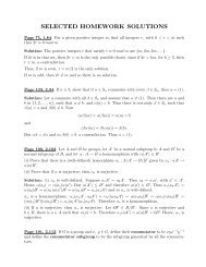
Figure D.1 breaks Iode down into its constituent modules. Each module
occurs as an m-file with the same name. For example, dfgui in the figure
means the file dfgui.m that comes as part of the Iode package. If you type
doctool(’guidoc’) at the Matlab prompt, you’ll see Figure D.1 in a Matlab
figure, and if you click on the name of a module, its help message will appear
in Matlab’s help window. This will give you an idea of what Iode’s modules
do and how they work together.
There are two kinds of module. The first kind are the GUI modules
and auxiliaries, providing the graphical user interface. The second (and
main) kind are the mathematical modules, which actually perform the calculations
needed to solve the differential equations numerically, and calculate
the Fourier coefficients numerically, and so on.
The mathematical moduleseuler.m andrk.m are particularly instructive
— they implement the Euler and Runge–Kutta methods for solving a first
order ODE. You can implement different solver methods yourself, as outlined
in Appendix C.
In order to develop a better understanding of what the various modules
do, you can look at the file doc.txt. Together with Figure D.1, it should
give you a rather complete picture of the structure of Iode. Another useful
file to look at is sample.m, which contains the transcript of a short Matlab
session that shows how to use the direction fields module and numerical
solvers without resorting to any menus.
37

38 APPENDIX D. STRUCTURE OF IODE
df
solplot
dfgui
rk
pp
euler
ppgui
trajplot
mvgui
ppaux
Iode −−− GUI Version
iodegui
sinef mixednd
mixeddn
cosef
dirichlet
periodicef
periodic
pdegui
wave
fsgui
mp
neumann
heat
fs
partialsum
coeff
trapsum
Figure D.1: Relationships between the most important modules of the GUI
version of Iode.
Any manual can only take you so far. If you have followed this manual
up to this point, you are ready to go exploring on your own. Good luck, and
have fun!