The Gixel Array Descriptor (GAD) for Multi-Modal Image Matching
The Gixel Array Descriptor (GAD) for Multi-Modal Image Matching
The Gixel Array Descriptor (GAD) for Multi-Modal Image Matching

You also want an ePaper? Increase the reach of your titles
YUMPU automatically turns print PDFs into web optimized ePapers that Google loves.
<strong>The</strong> <strong>Gixel</strong> <strong>Array</strong> <strong>Descriptor</strong> (<strong>GAD</strong>) <strong>for</strong> <strong>Multi</strong>-<strong>Modal</strong> <strong>Image</strong> <strong>Matching</strong><br />
Guan Pang<br />
University of Southern Cali<strong>for</strong>nia<br />
gpang@usc.edu<br />
Abstract<br />
Feature description and matching is a fundamental problem<br />
<strong>for</strong> many computer vision applications. However, most<br />
existing descriptors only work well on images of a single<br />
modality with similar texture. This paper presents a novel<br />
basic descriptor unit called a <strong>Gixel</strong>, which uses an additive<br />
scoring method to sample surrounding edge in<strong>for</strong>mation.<br />
Several <strong>Gixel</strong>s in a circular array create a powerful descriptor<br />
called the <strong>Gixel</strong> <strong>Array</strong> <strong>Descriptor</strong> (<strong>GAD</strong>), excelling<br />
in multi-modal image matching, especially when one of the<br />
images is edge-dominant with little texture. Experiments<br />
demonstrate the superiority of <strong>GAD</strong> on multi-modal matching,<br />
while maintaining a per<strong>for</strong>mance comparable to several<br />
state-of-the-art descriptors on single modality matching.<br />
1. Introduction<br />
Finding precise correspondences between image pairs is<br />
a fundamental task in many computer vision applications.<br />
A common solution is extracting dominant features to describe<br />
a complex scene, and comparing similarity between<br />
feature descriptors to determine the best correspondence.<br />
However, most descriptors only per<strong>for</strong>m well with images<br />
of the same modality. Successful matching depends on similar<br />
distributions of texture, intensity or gradient.<br />
<strong>Multi</strong>-modal images usually exhibit different patterns of<br />
gradient and intensity in<strong>for</strong>mation, making it hard <strong>for</strong> existing<br />
descriptors to find correspondences. Examples include<br />
matching images from SAR, visible light, infrared devices,<br />
Lidar sensors, etc. A special case in multi-modal matching<br />
is to match a traditional optical image to an edge-dominant<br />
image with little texture, such as matching optical images<br />
to 3D wireframes <strong>for</strong> model texturing, matching normal images<br />
to pictorial images <strong>for</strong> image retrieval, matching aerial<br />
images to maps <strong>for</strong> urban localization, etc. <strong>The</strong>se tasks are<br />
even harder <strong>for</strong> existing descriptors since they often don’t<br />
have any texture distribution in<strong>for</strong>mation.<br />
To match multi-modal images, especially edge-dominant<br />
images, we present a novel gradient-based descriptor unit<br />
1<br />
Ulrich Neumann<br />
University of Southern Cali<strong>for</strong>nia<br />
uneumann@graphics.usc.edu<br />
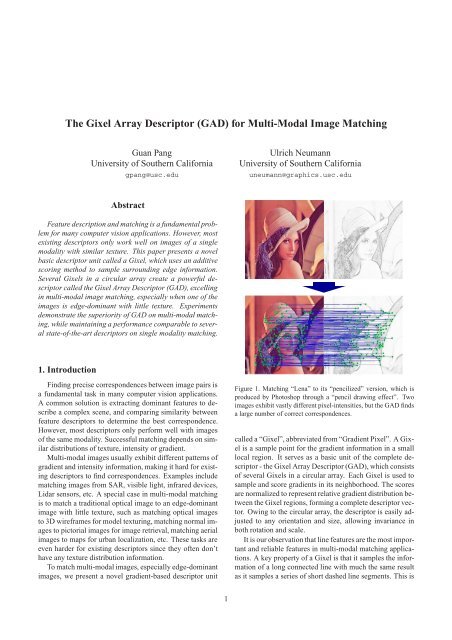
Figure 1. <strong>Matching</strong> “Lena” to its “pencilized” version, which is<br />
produced by Photoshop through a “pencil drawing effect”. Two<br />
images exhibit vastly different pixel-intensities, but the <strong>GAD</strong> finds<br />
a large number of correct correspondences.<br />
called a “<strong>Gixel</strong>”, abbreviated from “Gradient Pixel”. A <strong>Gixel</strong><br />
is a sample point <strong>for</strong> the gradient in<strong>for</strong>mation in a small<br />
local region. It serves as a basic unit of the complete descriptor<br />
- the <strong>Gixel</strong> <strong>Array</strong> <strong>Descriptor</strong> (<strong>GAD</strong>), which consists<br />
of several <strong>Gixel</strong>s in a circular array. Each <strong>Gixel</strong> is used to<br />
sample and score gradients in its neighborhood. <strong>The</strong> scores<br />
are normalized to represent relative gradient distribution between<br />
the <strong>Gixel</strong> regions, <strong>for</strong>ming a complete descriptor vector.<br />
Owing to the circular array, the descriptor is easily adjusted<br />
to any orientation and size, allowing invariance in<br />
both rotation and scale.<br />
It is our observation that line features are the most important<br />
and reliable features in multi-modal matching applications.<br />
A key property of a <strong>Gixel</strong> is that it samples the in<strong>for</strong>mation<br />
of a long connected line with much the same result<br />
as it samples a series of short dashed line segments. This is
achieved by an additive scoring method. <strong>The</strong> score obtained<br />
with small line segments of similar orientation and distance<br />
to the <strong>Gixel</strong> is similar to the score obtained from a long connected<br />
line of the same orientation and distance. In multimodal<br />
data, due to different sensor characteristics, line features<br />
may appear with gaps or zig-zag segments. <strong>Gixel</strong>’s<br />
additive scoring method samples broken or solid lines with<br />
similar scores. This is essential <strong>for</strong> multi-modal matching.<br />
Figure 1 shows an example matching result of the <strong>Gixel</strong>based<br />
descriptor, between an ordinary image and a “pencil<br />
drawing” stylized image.<br />
Our main contributions include:<br />
• We observe that line features are the most important<br />
and reliable features in many multi-modal matching<br />
applications.<br />
• We propose the <strong>Gixel</strong> <strong>Array</strong> <strong>Descriptor</strong> (<strong>GAD</strong>) to<br />
extract line features, and thus per<strong>for</strong>m robustly <strong>for</strong><br />
matching multi-model images, especially on edgedominant<br />
images with little texture.<br />
• We demonstrate that the <strong>GAD</strong> can achieve good<br />
matching per<strong>for</strong>mance in various multi-modal applications,<br />
while maintaining a per<strong>for</strong>mance comparable to<br />
several state-of-the-art descriptors on single modality<br />
matching.<br />
2. Related Work<br />
<strong>The</strong> existing keypoint descriptors can be roughly classified<br />
into two categories: <strong>The</strong> ones based on intensity or<br />
gradient distribution, and the ones based on pixel comparison<br />
or ordering.<br />
<strong>The</strong> distribution-based descriptors are more traditional,<br />
which can be dated back to the works of Zabih and Woodfill<br />
[3], Johnson and Hebert [4] and Belongie et al. [5]. An<br />
important representative descriptor in this category is SIFT<br />
(Scale-Invariant Feature Trans<strong>for</strong>m) [6], which coded orientation<br />
and location in<strong>for</strong>mation of gradients in the descriptor<br />
region into a histogram, weighted by magnitude. Ke<br />
and Sukthankar [7] reduced the complexity of SIFT with<br />
PCA, leading to PCA-SIFT which is faster but also less distinctive<br />
than SIFT. Mikolajczyk and Schmid [1] proved the<br />
great per<strong>for</strong>mance of SIFT, and proposed a new descriptor<br />
based on SIFT by changing its location grid and reducing<br />
redundancy through PCA. <strong>The</strong> resulting GLOH is more distinctive<br />
than SIFT, but at the same time more expensive to<br />
compute. Bay et al. [2] proposed SURF (Speeded-Up Robust<br />
Features), using integral images to reduce the computation<br />
time, while still retaining the same gradient distribution<br />
histograms of SIFT. SURF [2] has proved to be one of the<br />
best descriptors in various circumstances.<br />
Recently, comparison-based descriptors are attracting attention.<br />
<strong>The</strong>se descriptors use relative comparison or ordering<br />
result of pixel intensities rather than the original inten-<br />
sities, resulting in much more efficient descriptor computation,<br />
while still maintaining per<strong>for</strong>mance competitive to<br />
distribution-based descriptors such as SIFT or SURF. Tang<br />
et al. [10] proposed a 2D histogram in the intensity ordering<br />
and spatial sub-division spaces, resulting in a descriptor<br />
called OSID, invariant to complex brightness change as<br />
long as it’s monotonically increasing. Calonder et al. [8]<br />
proposed BRIEF, using a binary string consisting the results<br />
of pair-wise pixel intensity comparison at pre-determined<br />
location, which is very fast in descriptor extraction and<br />
matching, but also very susceptible to rotation and scale<br />
changes. Rublee et al. [9] improved BRIEF into ORB (Oriented<br />
BRIEF), so that it’s rotation invariant and also resistant<br />
to noise. <strong>The</strong>re are several other descriptors within this<br />
category [11][12][13]. However, this type of descriptor relies<br />
heavily on extensive texture, thus they are not suitable<br />
<strong>for</strong> multi-modal matching. <strong>The</strong> proposed <strong>Gixel</strong>-based descriptor<br />
belongs to the distribution-based category.<br />
3. Introduction to <strong>Gixel</strong><br />
A <strong>Gixel</strong>, or “Gradient Pixel”, is a sample point <strong>for</strong> the<br />
gradient in<strong>for</strong>mation in a small local region on an image.<br />
A traditional Pixel would capture the pictorial in<strong>for</strong>mation<br />
of its neighborhood, and produce an intensity value or a 3D<br />
vector (R, G, B). Likewise, a <strong>Gixel</strong> would extract and summarize<br />
the gradient in<strong>for</strong>mation of its neighborhood. All<br />
line segments or pixelized gradients within the neighborhood<br />
of a <strong>Gixel</strong> are sampled (or scored) to produce a 2D<br />
vector of both x and y gradient data.<br />
3.1. Additive Edge Scoring<br />
For each line segment or pixelized gradient (a pixel gradient<br />
is considered as a line segment of length 1), a <strong>Gixel</strong><br />
creates a score, which encodes three elements of in<strong>for</strong>mation:<br />
orientation, length, and distance to the <strong>Gixel</strong>. <strong>The</strong><br />
longer a line segment is, the higher it is scored. Similarly,<br />
the nearer a line segment is to the <strong>Gixel</strong>, the higher it is scored.<br />
<strong>The</strong> score is then divided into x and y components<br />
according to the orientation of the line segment or gradient.<br />
In addition, sensor noise or inaccurate edge detection<br />
usually results in small gaps, zigzags, or other artifacts along<br />
the line, as shown in Fig.2(a, b). <strong>The</strong> design of the<br />
scoring function makes it additive, so that a sequence of<br />
short line segments achieves a similar score as a long connected<br />
line, as shown in Fig.2(c).<br />
<strong>The</strong> function f(x) = 1/(1+x): has the properties that<br />
f(0) = 1, f(+∞) = 0, and f(x) decreases as the input<br />
valuex increases.<br />
<strong>The</strong> scoring function is constructed from f(x). Given<br />
a line segment’s length l, and distance to the <strong>Gixel</strong> d, the<br />
score is defined as:<br />
Score(l,d) = f(d)−f(d+l) = 1<br />
1+d −<br />
1<br />
1+d+l (1)
Figure 2. (a) Small gap and zigzag artifacts appeared in many edge images. (b) Small gap appeared in edge detection. (c) Additive edge<br />
scoring makes short dashed line segments achieve a similar score as a long connected line. (d) Score of a line segment given its length l<br />
and distance d to the <strong>Gixel</strong>. (e) Illustration of Manhattan distance.<br />
Figure 2(d) illustrates the scoring function. Since f(x) is<br />
monotonically decreasing, Score(l,d) should increase as l<br />
increases. Moreover, f ′ (x) is always negative and monotonically<br />
increasing, making Score(l,d) decreases as d increases.<br />
<strong>The</strong> score is then broken into x and y components,<br />
reflecting the orientation of the line segment.<br />
Finally, to achieve the property that short dashed line<br />
segments are scored similarly to a long connected line, we<br />
use Manhattan distance <strong>for</strong> d instead of Euclidian distance,<br />
which is defined as the distance from the <strong>Gixel</strong> to the intersection<br />
point between the <strong>Gixel</strong> and the line, plus the distance<br />
from the intersection point to the nearest point on the<br />
line segment (0 if the intersection point is on the line segment).<br />
It might seem that using Manhattan distance causes<br />
line segments pointing towards the <strong>Gixel</strong> to be scored higher<br />
than those perpendicular ones. This is actually intended, so<br />
when a <strong>Gixel</strong> lies along the extension of a line segment, that<br />
line should have more importance to the <strong>Gixel</strong> score. Thus<br />
<strong>Gixel</strong>s will also differentiate lines by their orientations.<br />
For example, as shown in Fig.2(e),AB is a line segment,<br />
C and C ′ are two points on AB near each other, G is the<br />
<strong>Gixel</strong>, and F is the intersection point from G to AB. We<br />
want to show that AB and AC + C ′ B contribute similar<br />
scores to the <strong>Gixel</strong>G:<br />
ScoreAB = Score(AB,GF +FA)<br />
ScoreAC +ScoreC ′ B<br />
= f(GF +FA)−f(GF +FB)<br />
= Score(AC,GF +FA)+Score(C ′ B,GF +FC ′ )<br />
= f(GF +FA)−f(GF +FC)<br />
+f(GF +FC ′ )−f(GF +FB)<br />
≈ f(GF +FA)−f(GF +FB) = ScoreAB<br />
<strong>The</strong> two short line segments AC and C ′ B will be scored<br />
similarly to the whole line segmentAB, overcoming the impact<br />
of the gapCC ′ . This way, we aggregate the impact of<br />
multiple end-to-end short segments <strong>for</strong> improved matching<br />
of multi-modal images. Lastly, note that the scoring system<br />
is smooth and does not introduce thresholds or discontinuities<br />
as a function of segment parameters.<br />
(2)<br />
(3)<br />
3.2. Circular <strong>Gixel</strong> <strong>Array</strong><br />
All line segments or pixelized gradients within the neighborhood<br />
of a <strong>Gixel</strong> will be scored, summed up, and split<br />
into a 2-D vector with x and y components to encode orientation<br />
in<strong>for</strong>mation. However, a single 2D vector will not<br />
provide enough discriminative power <strong>for</strong> a complex image.<br />
<strong>The</strong>re<strong>for</strong>e, <strong>for</strong> a complete descriptor, we put several <strong>Gixel</strong>s<br />
in a region, compute their gradient scores individually, and<br />
connect their scores into a larger vector. <strong>The</strong> vector is then<br />
normalized to encode relative gradient strength distribution<br />
among the <strong>Gixel</strong>s, as well as reduce the effect of illumination<br />
change.<br />
While many <strong>Gixel</strong> array distributions are possible, we<br />
put the <strong>Gixel</strong>s in a circular array to <strong>for</strong>m the complete descriptor,<br />
which is named <strong>Gixel</strong> <strong>Array</strong> <strong>Descriptor</strong> (<strong>GAD</strong>),<br />
as shown in Fig.3(a). <strong>The</strong> circular array is very helpful in<br />
achieving rotation and scale invariance (Sec.5.3). <strong>The</strong> <strong>Gixel</strong>s<br />
are placed on concentric circles with different radii extending<br />
from the center <strong>Gixel</strong>. <strong>The</strong>re are three parameters<br />
involved: the number of circles, the number of <strong>Gixel</strong>s on<br />
each circle, and the distance between each circle (Figure 3<br />
shows an example of 2 circles and 8 <strong>Gixel</strong>s on each circle).<br />
<strong>The</strong> circular layout is similar to the DAISY descriptor [14],<br />
but the computation of the two descriptors are completely<br />
different since we aim at different applications.<br />
Figure 3. (a) Circular <strong>Gixel</strong> array - each yellow point is a <strong>Gixel</strong>.<br />
(b) A <strong>Gixel</strong> array can be adjusted <strong>for</strong> rotation and scale invariance.
<strong>The</strong> array parameters are determined empirically, but are<br />
not critical in our experience. A dense <strong>Gixel</strong> array may lead<br />
to redundancy and unnecessary complexity, as <strong>Gixel</strong>s close<br />
to each other will sample similar gradient in<strong>for</strong>mation. On<br />
the other hand, too few or too sparse a <strong>Gixel</strong> array will reduce<br />
the discriminative power of the descriptor, and result<br />
in low feature dimension or low correlation between <strong>Gixel</strong>s.<br />
In our experiments, we use fixed parameters of 3 circles, 8<br />
<strong>Gixel</strong>s on each circle, and the distance between each circle<br />
is 50 pixels (which means the radius is 50, 100, 150 from<br />
the center <strong>Gixel</strong>). Thus there are 3 ∗8+1 = 25 <strong>Gixel</strong>s in<br />
total, resulting in a feature dimension of 50.<br />
A circular <strong>Gixel</strong> array also has several other benefits.<br />
It’s easy to generate and reproduce. Each <strong>Gixel</strong> in the array<br />
samples the region evenly. Most importantly, it can be<br />
adapted to achieve rotation and scale invariance by rotating<br />
<strong>Gixel</strong>s on the circle and adjusting circle radius (refer to<br />
Sec.5.3), as shown in Fig.3(b).<br />
3.3. <strong>Descriptor</strong> Localization and <strong>Matching</strong><br />
Unlike descriptors such as SIFT or SURF, which require<br />
a keypoint detection step, <strong>GAD</strong> can be computed with any<br />
detector or at any arbitrary location, while still maintaining<br />
good per<strong>for</strong>mance even under multi-modal situations, due<br />
to its smoothness property (Sec.4.1). In practice we find<br />
that a simple keypoint detection step like the Harris corner<br />
detector can be used to identify areas with gradients to<br />
speed up the matching process.<br />
<strong>The</strong> distance between two descriptors is computed as the<br />
square root of squared difference of the two vectors. Two<br />
descriptors on two images are considered matched if the<br />
nearest neighbor distance ratio [1] is larger than a threshold.<br />
<strong>The</strong> nearest neighbor distance ratio is defined as the<br />
ratio of distance between the first and the second nearest<br />
neighbors.<br />
4. Analysis of Advantages<br />
4.1. Smoothness<br />
<strong>The</strong> design of <strong>GAD</strong> takes special care to achieve its<br />
smoothness property, both in how gradients are scored, and<br />
in how the neighborhood size of each <strong>Gixel</strong> is determined.<br />
<strong>The</strong> scoring function is defined as a smooth function monotonically<br />
decreasing with length and distance. <strong>The</strong> neighborhood<br />
of each <strong>Gixel</strong> is cut off smoothly, so that the score<br />
is negligible at its boundary, resulting in a circular neighborhood<br />
of 50-pixel radius. A small change in a line segment’s<br />
length, orientation, distance or the location of a <strong>Gixel</strong><br />
sample will only result in a small change in the descriptor.<br />
Moreover, the additive scoring property of a <strong>Gixel</strong> also contributes<br />
to the smoothness by alleviating the impact of noise<br />
and line gaps.<br />
When matching images of a single modality, it is desir-<br />
Figure 4. <strong>Descriptor</strong> similarity score distribution when moving<br />
keypoint in the neighborhood. (a) <strong>GAD</strong>; (b) SURF.<br />
able to use a score function with a sharp peak. Smoothness<br />
may not be an important issue in this case. However,<br />
<strong>for</strong> multi-modal matching, even corresponding regions may<br />
not have exactly the same intensity or gradient distribution.<br />
<strong>The</strong> smoothness property of a <strong>Gixel</strong> makes it more robust<br />
to noise and thus better suited <strong>for</strong> multi-modal applications.<br />
In addition, a <strong>Gixel</strong>-based descriptor relies less on accurate<br />
selection of a keypoint position. This means that keypoint<br />
selection is not critical. Even when keypoints have small<br />
offsets between two images, which is common in multimodal<br />
matching, <strong>Gixel</strong>s can still match them correctly.<br />
On the other hand, traditional descriptors doesn’t exhibit<br />
smoothness, as they usually divides pixels and gradients into<br />
small bins and makes numerous binary decision or selections.<br />
Comparison-based descriptors are even worse, because<br />
noise or keypoint variations might change the pixel<br />
position and ordering completely.<br />
Figure 4 shows the distribution of matching similarity<br />
score between two descriptors in corresponding regions (of<br />
Fig.5), when one of the descriptor is moving. <strong>The</strong> <strong>Gixel</strong> descriptor<br />
(Fig.4(a)) demonstrates better smoothness and distinctiveness<br />
(single peak) than SURF (Fig.4(b)).<br />
4.2. <strong>Multi</strong>-<strong>Modal</strong> <strong>Matching</strong><br />
Line features are the most important and sometimes the<br />
only available feature in multi-modal matching problems.<br />
Each <strong>Gixel</strong> in the descriptor array samples and scores the<br />
line features in its neighborhood from a different distance<br />
and orientation. In other words, the <strong>Gixel</strong>s sample overlapping<br />
regions of edge in<strong>for</strong>mation, but from different locations.<br />
This spatial distribution of samples imparts the final<br />
descriptor with its discriminating power.<br />
On the other hand, traditional distribution-based descriptors<br />
tend to break a long line feature into individual grid or<br />
bin contributions. Noisy line rendering and detection might<br />
impact the distribution statistics heavily, making the matching<br />
process unreliable.<br />
<strong>Descriptor</strong>s based on pixel-wise comparison may also<br />
suffer in multi-modal matching, as the lack of texture will<br />
not provide enough distinctive pixel pairs to work robustly.
Figure 5. Per<strong>for</strong>mance comparison between <strong>GAD</strong> and SIFT, SURF, BRIEF, ORB when matching aerial images to building rooftop outlines<br />
generated from 3D models <strong>for</strong> urban models texturing. (a) <strong>Matching</strong> with SIFT. (b) <strong>Matching</strong> with SURF. (c) <strong>Matching</strong> with BRIEF.<br />
(d) <strong>Matching</strong> with ORB. (e) <strong>Matching</strong> with <strong>GAD</strong> (no RANSAC). (f) recall vs. 1 − precision curves. (g) <strong>Matching</strong> with <strong>GAD</strong> (after<br />
RANSAC). (h) Registered aerial image and 3D wireframes using <strong>GAD</strong>.<br />
5. Experiments<br />
5.1. Evaluation Method<br />
<strong>The</strong> proposed descriptor is evaluated on both public test<br />
data and multi-modal data of our own. For public test data,<br />
we choose the well-known dataset provided by Mikolajczyk<br />
and Schmid [1], which is a standard dataset <strong>for</strong> descriptor<br />
evaluation used by many researchers. It contains several<br />
image series with various trans<strong>for</strong>mation, including zoom<br />
and rotation (Boat), viewpoint change (Graffiti), illumination<br />
change (Leuven), JPEG compression (Ubc). On the<br />
other hand, multi-modal matching is still a relatively new<br />
research area, so there is no established test dataset yet. We<br />
use some of our own data to evaluate the per<strong>for</strong>mance of<br />
<strong>GAD</strong>. <strong>The</strong>se data sets will be posted online <strong>for</strong> others to<br />
use in comparisons.<br />
We use SIFT [6], SURF [2], BRIEF [8] and ORB [9]<br />
<strong>for</strong> comparison during our evaluation. <strong>The</strong>y are good representatives<br />
of existing descriptors, since they cover both<br />
categories described in Sec.2, and are usually compared to<br />
other descriptors, producing similar per<strong>for</strong>mance. To make<br />
fair comparisons, we also use SURF’s feature detector to<br />
determine keypoints locations <strong>for</strong> <strong>GAD</strong>. After feature extraction,<br />
all descriptors are put through the same matching<br />
process to determine matched pairs (Note that <strong>GAD</strong>, SIFT,<br />
SURF all use L2 norm distance, but BRIEF and ORB have<br />
to use hamming distance). We use the latest build of Open-<br />
SURF 1 <strong>for</strong> implementation of SURF. For SIFT, BRIEF and<br />
ORB, we use the latest version of OpenCV 2 . Edges are extracted<br />
by a Canny detector.<br />
To evaluate the per<strong>for</strong>mance objectively, We computed<br />
recall and 1 − precision based on the number of correct<br />
matches, false matches, and total correspondence [1]. Two<br />
keypoints are correctly matched if the distance between<br />
their location under the ground-truth trans<strong>for</strong>mation is below<br />
a certain threshold. Correspondence is defined as the<br />
total number of possible correct matches. By changing the<br />
matching threshold, we can obtain different values ofrecall<br />
and1−precision. A per<strong>for</strong>mance curve is then plotted as<br />
recall versus1−precision.<br />
5.2. <strong>Multi</strong>-<strong>Modal</strong> <strong>Matching</strong><br />
Figure 5 shows an important matching problem we encountered<br />
during our research. We need to match aerial images<br />
to 3D wireframes <strong>for</strong> urban models texturing. One of<br />
the images contains only the building rooftop outlines generated<br />
from 3D models, which is a binary image without<br />
any intensity or texture in<strong>for</strong>mation. Figure 5(a,b,c,d) are<br />
the matching results of SIFT, SURF, BRIEF, ORB, respectively.<br />
None of these establish enough good matches to even<br />
apply RANSAC. Figure 5(e) shows the matching result ob-<br />
1 http://www.chrisevansdev.com/computer-vision-opensurf.html<br />
2 http://opencv.willowgarage.com/wiki/
Figure 6. Per<strong>for</strong>mance comparison when matching a photo and a drawing. (a) <strong>Matching</strong> with SIFT. (b) <strong>Matching</strong> with SURF. (c) <strong>Matching</strong><br />
with BRIEF. (d) <strong>Matching</strong> with ORB. (e) <strong>Matching</strong> with <strong>GAD</strong>. (f)recall vs. 1−precision curves.<br />
Figure 7. Per<strong>for</strong>mance comparison when matching an intensity image and a depth image. (a) <strong>Matching</strong> with SIFT. (b) <strong>Matching</strong> with<br />
SURF. (c) <strong>Matching</strong> with BRIEF. (d) <strong>Matching</strong> with ORB. (e) <strong>Matching</strong> with <strong>GAD</strong>. (f)recall vs. 1−precision curves.<br />
tained by <strong>GAD</strong>. Most matches are correct, thus the incorrect<br />
ones can be filtered out via RANSAC , as shown in Fig.5(g).<br />
Using the refined matches, we can estimate the true trans<strong>for</strong>mation<br />
homography between the two images, and reproject<br />
the aerial images onto the 3D wireframes <strong>for</strong> texturing,<br />
as shown in Fig.5(h). Figure 5(f) provides the recall vs.<br />
1 − precision curve comparison, which shows that traditional<br />
descriptors barely works with different texture distribution<br />
patterns, as can be seen from their low recall value<br />
in the curves, while <strong>GAD</strong> exhibit robust per<strong>for</strong>mance.<br />
Figure 6 demonstrates another possible application of<br />
multi-modal matching, to match an ordinary image with an<br />
artistic image <strong>for</strong> image retrieval. One image is a photo of<br />
the Statue of Liberty, and the other one is a drawing of the<br />
Statue. Figure 6(a,b,c,d) are the matching results of SIFT,<br />
SURF, BRIEF, ORB, respectively. None of them exhibits<br />
many good matches, while <strong>GAD</strong> can find a good number<br />
of correct matches, in spite of completely different image<br />
modality and the slight viewpoint change between the<br />
two images, as shown in Fig.6(e). Figure 6(f) provides the<br />
recall vs. 1−precision curve comparison.<br />
Figure 7 shows two images taken on the same area, but
Figure 8. Potential multi-modal matching applications of the<br />
<strong>GAD</strong>. (a) <strong>Matching</strong> maps to aerial images. (b) Medical image<br />
registration.<br />
one is an intensity image, and the other is a depth image,<br />
with visibly different visual patterns. Figure 7(a,b,c,d) are<br />
the matching results of SIFT, SURF, BRIEF, ORB, respectively.<br />
None of them manages to find enough correct matches,<br />
if any. On the other hand, <strong>GAD</strong> is able to find many<br />
correct matches, as shown in Fig.7(e). Figure 7(f) provides<br />
therecall vs. 1−precision curve comparison.<br />
<strong>The</strong> <strong>GAD</strong> has many other potential multi-modal matching<br />
applications, such as matching maps to aerial images, or<br />
medical image registration [15], as shown in Fig.8(a,b).<br />
5.3. Rotation and Scale Invariance<br />
<strong>The</strong> <strong>GAD</strong> is easily adjusted to achieve both rotation and<br />
scale invariance. <strong>The</strong> smoothness property of <strong>Gixel</strong>s introduced<br />
in Sec.4.1 makes it robust to small scale or rotation<br />
changes, as shown in Fig.9(a). This allows a search <strong>for</strong> scale<br />
and rotation changes. <strong>The</strong> <strong>Gixel</strong> sample point positions<br />
are simply adjusted <strong>for</strong> each search step in scale or rotation.<br />
As introduced in Sec.3.2, <strong>Gixel</strong>s are organized in a circular<br />
array, with several <strong>Gixel</strong>s placed evenly on each circle.<br />
To align the descriptor into a new orientation, we just rotate<br />
the array w.r.t. the center <strong>Gixel</strong>, so that all <strong>Gixel</strong>s are still<br />
sampling corresponding regions when the center position is<br />
matched. In addition, <strong>for</strong> each <strong>Gixel</strong>, the score in both x and<br />
y components(xold,yold) is converted through the triangle<br />
function trans<strong>for</strong>mation to account <strong>for</strong> the rotation change<br />
into(xnew,ynew):<br />
<br />
xnew = |xold ×cosα+yold ×sinα|<br />
(4)<br />
ynew = |yold ×cosα−xold ×sinα|<br />
Scale invariance can be achieved similarly. First adjust<br />
the radius of each circle in the circular <strong>for</strong>mation according<br />
to the scale. <strong>The</strong>n adjust size of the neighborhood <strong>for</strong><br />
Figure 9. <strong>Matching</strong> per<strong>for</strong>mance of <strong>GAD</strong> with rotation and scale<br />
changes under multi-modal situations. (Curves comparison is not<br />
included since other descriptors barely work in multi-modality, as<br />
Sec.5.2 already showed.) (a) <strong>Matching</strong> between image 1 and 2<br />
from the “Graffiti” series [1], while one of the images are rendered<br />
with a “glowing edges effect”. (b) <strong>Matching</strong> between image 1 and<br />
4 from the “Boat” series [1], while one of the images are rendered<br />
with a “pencil drawing effect”.<br />
each <strong>Gixel</strong> so it covers the same region under different image<br />
size. Finally, distance and length value of all gradients<br />
within the neighborhood are also scaled linearly. It should<br />
be noted that we are not just compensating <strong>for</strong> a known<br />
rotation or scale change. Instead, we search <strong>for</strong> possible<br />
changes, and compensate <strong>for</strong> each searched change using<br />
the methods described above.<br />
Figure 9(b) uses two images from the “Boat” series [1]<br />
with both rotation and scale changes, though the 2nd one is<br />
further rendered with a “pencil drawing effect” via Photoshop.<br />
<strong>GAD</strong> exhibits rotation and scale invariance by finding<br />
a good number of correct matches.<br />
5.4. Public Dataset<br />
Figure 9(a,b) both come from the public dataset [1],<br />
where <strong>GAD</strong> can achieve good per<strong>for</strong>mance even under<br />
multi-modal situations. We present two more examples in<br />
Fig.10(a,b), the “Ubc” series with JPEG compression and<br />
the “Leuven” series with illumination change, again both<br />
from the public dataset [1]. Due to space limitation, the<br />
matching results of other descriptors are not listed here (except<br />
their curves). <strong>The</strong>y can be found in previous literatures.<br />
Figure 10(a) shows that the <strong>GAD</strong> outper<strong>for</strong>ms other descriptors<br />
on the “Ubc” data with JPEG compression. A<br />
possible explanation is that matching images under JPEG<br />
compression to normal images is similar to a multi-modal<br />
problem, as JPEG compression will produce more “bloblike”<br />
areas with quantization edges and deteriorated texture<br />
quality. <strong>The</strong> smoothness property (Sec.4.1) of <strong>Gixel</strong>s also
Figure 10. More results <strong>for</strong> matching with <strong>GAD</strong> (left) and recall vs. 1 − precision curve comparison (right). (a) <strong>Matching</strong> with JPEG<br />
compression (image 1 and 2 from the “Ubc” series [1]) (b) <strong>Matching</strong> with illumination change (image 1 and 4 from the “Leuven” series [1])<br />
likely helps in reducing the impact of JPEG compression.<br />
In Fig.10(b) with illumination change, the <strong>GAD</strong> has a recall<br />
rate slightly inferior to other descriptors, but still finds<br />
a large number of correct matches with almost no errors.<br />
5.5. Processing Time<br />
<strong>GAD</strong>’s computation process is time-consuming compared<br />
to state-of-the-art descriptors, but no ef<strong>for</strong>ts at optimization<br />
have been made yet. For examples, Fig.1 (size<br />
512x512) takes <strong>GAD</strong> 8.9 seconds, while SURF needs 0.7s;<br />
Fig.10(b) (size 900x600) takes <strong>GAD</strong> 19.5s, while SURF<br />
needs 1.3s. At this point, speed is not a primary concern in<br />
our research, but we’ll pursue optimizations in future work.<br />
6. Conclusion<br />
We introduce a novel descriptor unit called a <strong>Gixel</strong>,<br />
which uses an additive scoring method to extract surrounding<br />
edge in<strong>for</strong>mation. We show that a circular array of <strong>Gixel</strong>s<br />
will sample edge in<strong>for</strong>mation in overlapping regions to<br />
make the descriptor more discriminative and it can be invariant<br />
to rotation and scale. Experiments demonstrate the<br />
superiority of the <strong>Gixel</strong> array descriptor (<strong>GAD</strong>) <strong>for</strong> multimodal<br />
matching, while maintaining a per<strong>for</strong>mance comparable<br />
to state-of-the-art descriptors on traditional single<br />
modality matching.<br />
<strong>The</strong> <strong>GAD</strong> still has some limitations in its current development<br />
status. We have put little ef<strong>for</strong>t into optimization,<br />
so the run time is slow. In addition, though <strong>GAD</strong> exhibits<br />
rotation and scale invariance, large viewpoint changes may<br />
reduce per<strong>for</strong>mance, and we have not addressed that issue<br />
yet. Finally, as a feature built sole on edges, <strong>GAD</strong> may not<br />
per<strong>for</strong>m well in situations where edges are rare. <strong>The</strong>se issues<br />
will be investigated sin our future work.<br />
References<br />
[1] K. Mikolajczyk and C. Schmid. A per<strong>for</strong>mance evaluation of<br />
local descriptors. IEEE Transactions on Pattern Analysis and<br />
Machine Intelligence, 27(10):1615–1630, 2005. 2, 4, 5, 7, 8<br />
[2] H. Bay, A. Ess, T. Tuytelaars, L. Van Gool. SURF: Speeded<br />
Up Robust Features. Computer Vision and <strong>Image</strong> Understanding,<br />
110(3):346–359, 2008. 2, 5<br />
[3] R. Zabih and J. Woodfill. Non-parametric local trans<strong>for</strong>ms <strong>for</strong><br />
computing visual correspondance. Proceedings of the European<br />
Conference on Computer Vision, pp.151–158, 1994. 2<br />
[4] A. Johnson and M. Hebert. Object recognition by matching<br />
oriented points. Proceedings of the IEEE Conference on Computer<br />
Vision and Pattern Recognition, pp.684–689, 1997. 2<br />
[5] S. Belongie, J. Malik, and J. Puzicha. Shape matching and<br />
object recognition using shape contexts. IEEE Transactions<br />
on Pattern Analysis and Machine Intelligence, 24(4):509–522,<br />
2002. 2<br />
[6] D. Lowe. Distinctive image features from scale-invariant keypoints.<br />
International Journal of Computer Vision, 60(2):91–<br />
110, 2004. 2, 5<br />
[7] Y. Ke and R. Sukthankar. PCA-SIFT: A more distinctive representation<br />
<strong>for</strong> local image descriptors. Proceedings of the<br />
IEEE Conference on Computer Vision and Pattern Recognition,<br />
pp.511–517, 2004. 2<br />
[8] M. Calonder, V. Lepetit, C. Strecha, and P. Fua. BRIEF: Binary<br />
Robust Independent Elementary Features. Proceedings of<br />
the European Conference on Computer Vision, 2010. 2, 5<br />
[9] E. Rublee, V. Rabaud, K. Konolige, G. Bradski. ORB: an efficient<br />
alternative to SIFT or SURF. Proceedings of the IEEE<br />
International Conference on Computer Vision, 2011. 2, 5<br />
[10] F. Tang, S. H. Lim, N. L. Chang , H. Tao. A novel feature<br />
descriptor invariant to complex brightness changes. Proceedings<br />
of the IEEE Conference on Computer Vision and Pattern<br />
Recognition, pp.2631–2638, 2009. 2<br />
[11] A. Bosch, A. Zisserman, and X. Munoz. <strong>Image</strong> classification<br />
using random <strong>for</strong>ests and ferns. Proceedings of the IEEE<br />
International Conference on Computer Vision, 2007. 2<br />
[12] E. Shechtman and M. Irani. <strong>Matching</strong> local self-similarities<br />
across images and videos. Proceedings of the IEEE Conference<br />
on Computer Vision and Pattern Recognition, 2007. 2<br />
[13] S. Leutenegger, M. Chli and R. Siegwart. BRISK: Binary<br />
Robust Invariant Scalable Keypoints, Proceedings of the IEEE<br />
International Conference on Computer Vision, 2011. 2<br />
[14] S. Winder, G. Hua, M. Brown. Picking the best DAISY. Proceedings<br />
of the IEEE Conference on Computer Vision and<br />
Pattern Recognition, pp.178-185, 2009. 3<br />
[15] G. Yang, C. V. Stewart, M. Sofka, C. L. Tsai. Registration of<br />
Challenging <strong>Image</strong> Pairs: Initialization, Estimation, and Decision.<br />
IEEE Transactions on Pattern Analysis and Machine<br />
Intelligence, 29(11):1973–1989, 2007. 7