Comparison of Axial Dispersion and Tanks-in-Series Models for ...

Comparison of Axial Dispersion and Tanks-in-Series Models for
Simulating the Performance of Enzyme Reactors
Ibrahim M. Abu-Reesh* and Basel F. Abu-Sharkh
Chemical Engineering Department, King Fahd University of Petroleum & Minerals,
Dhahran 31261, Saudi Arabia
A comparison of two modeling approaches for simulating the performance of enzyme reactors
using the axial dispersion and tanks-in-series models is described. The two modeling approaches
are compared for the steady-state performance of enzyme reactors assuming Michaelis-Menten
kinetics with competitive product inhibition. The performance of the reactors is described in
terms of substrate conversion and yield. The equation Pe ) 2(N - 1) is used to correlate the
parameter of the dispersion model (Pe) with that of the tanks-in-series model (N) for the entire
range of dispersion from plug flow to CSTR. The predictions of the two models agree well,
especially at low dimensionless residence times and high Peclet numbers. Practically, the
predictions of the two models are essentially equivalent when the above equation is used to
relate their two parameters. However, the tanks-in-series model is simpler and has computational
advantages over the dispersion model, although its physical basis is not as clear as that of the
dispersion model. Lactose hydrolysis by the enzyme -galactosidase, which exhibits Michaelis-
Menten kinetics with competitive product inhibition, is used as a model system in this study.
The kinetic parameters for lactose hydrolysis are obtained from the literature.
Introduction
The continuous stirred tank reactor (CSTR) and plugflow
reactor (PFR) are two different ideal reactor models
that are used for the description of flow reactors. The
CSTR assumes perfect mixing, whereas the PFR assumes
no mixing. No real reactor has precisely the
characteristics of either of the two ideal reactors. The
axial dispersion model (ADM) and tanks-in-series model
(TISM) are one-parameter models that describe partially
mixed reactors with a finite level of mixing, which
cannot be described by either of the two ideal reactor
models. The ADM is characterized by the Peclet number
(Pe), which represents all of the effects that cause
deviations from ideal PFR behavior, such as nonuniform
velocity profiles or eddies. The Pe number is the single
parameter in this model. As Pe increases from 0 to ∞,
the flow pattern in the reactor changes from complete
mixing (CSTR) to no mixing (PFR). The ADM requires
solution of a second-order differential equation to compute
the steady-state conversion. In addition, this model
gives different results for different boundary conditions.
In the TISM, the nonideal reactor is considered as being
made up of a cascade of N equal-sized CSTRs arranged
in series. N is the single parameter in this model. As N
increases from 1 to ∞, the flow pattern in the reactor
changes from complete mixing (CSTR) to no mixing
(PFR). Although the physical basis of the TISM is not
as clear as that of the ADM, the TISM is simple and
can be used with any kinetic equation. The steady-state
mathematical model of the TISM requires the solution
of algebraic equations instead of a differential equation.
The main defect of the TISM is that N takes only integer
values. This limitation can be removed by using either
* To whom correspondence should be addressed. Current
address: Dr. Ibrahim M. Abu-Reesh, Chemical Engineering
Department, The University of Jordan, Amman 11942, Jordan.
E-mail: abureesh@ju.edu.jo.
Ind. Eng. Chem. Res. 2003, 42, 5495-5505
5495
the gamma function model 1 or the fractional tank
model. 2 When N is allowed to take noninteger values,
then the computational advantage is lost. Although the
ADM and TISM are rather similar in many ways, there
is no one exact way to compare them. However, the two
models can be compared quantitatively by equating
their variances. This leads to a relationship between
their two parameters, Pe and N.
In the literature, there appears to be a lack of
agreement in utilizing the TISM and ADM in the
modeling of reactor systems including enzyme reactors,
which have growing industrial applications. Kobayashi
and Moo-Young (1971) 3 were the first to apply the
dispersion model to immobilized enzyme reactors. Some
authors 4 have pointed out that the ADM provides a
satisfactory description only of mixing that does not
deviate significantly from plug-flow behavior. Others 5
have emphasized that the application of the ADM for
Pe values of less than 10 is not advised and, in this
range, the TISM is more adequate. Turner and Mills
(1990) 6 reported that the TISM is more realistic and
advantageous compared to the ADM for simulating the
performance of Fischer-Tropsch slurry bubble column
reactors. Lee et al. 7 recommended a two-CSTRs-in-series
model to represent activated sludge processes for treating
municipal wastewater. Nardi et al. 8 showed that
the single-parameter models (ADM and TISM) satisfactorily
represent the flow pattern in horizontal flow
anaerobic immobilized sludge reactors. Poughon et al. 9
described the hydrodynamics of a nitrifying fixed-bed
column using a model including N tanks in series with
back-mixing. Komolprasert and Ofoli 10 showed that the
ADM is suitable for predicting the extent of starch
liquefaction by B. licheniformis R-amylase during reactive
extrusion. Using first-order enzyme kinetics, Komolprasert
and Ofoli 10 reported that the ADM is suitable
for analysis of enzymatic reactions up to 30%
conversion.
10.1021/ie030131j CCC: $25.00 © 2003 American Chemical Society
Published on Web 10/03/2003

5496 Ind. Eng. Chem. Res., Vol. 42, No. 22, 2003
Using the equation Pe ) 2(N - 1) to relate the
parameters of the two models, Elgeti 11 found good
agreement between a pipe flow reactor and a series of
ideally mixed reactors for first-order, second-order, and
first-order successive reactions. Elgeti 11 showed that the
equation Pe ) 2(N - 1) has a good theoretical basis.
Others 12,13 also have used the same equation. Van
Hasselt et al. 14 showed that, for the three levels of a
porosity reactor, both the gas and liquid residence time
distributions can be predicted with the TISM. Comparisons
of the ADM and TISM by matching the variances
led to a relationship between Pe and N. For small
deviations from the PFR, the Pe number was found to
be equal to 2N, whereas for the whole range of dispersion,
the equation Pe ) 2(N - 1) was used. Ponzi and
Gonzalez 15 compared the ADM and TISM for a firstorder
reversible reaction using the same conversion and
the same start-up time. Good agreement was found,
especially at low Damkohler numbers and high Peclet
numbers. In a recent paper, Dommeti and Balakotaiah 16
showed that there is an upper bound on the Damkohler
number at which the predictions of the ADM and TISM
begin to diverge. They derived an equation for this
upper bound of the Damkohler number for different
kinetic models. The objective of this work is to compare
the predictions of the ADM and TISM for the performance
of enzyme reactors. Reactor conversion and yield
are determined for enzyme reactions described by
Michaelis-Menten kinetics with competitive product
inhibition. This study discusses the conditions under
which the two models agree for predicting the performance
of enzyme reactors. The equation Pe ) 2(N - 1)
is used to relate the parameters of the two models. Milk
(or whey) lactose conversion to glucose and galactose
by the enzyme -galactosidase is investigated using the
two modeling approaches.
Model Development
Axial Dispersion Model. Consider an enzyme reactor
of length L and fluid velocity u. Assuming axial
dispersion, the steady-state material balance of the
substrate (with concentration S) in the liquid is given
by17 d
Dz 2 S dS
- u - [-R(S,P)] ) 0 (1)
2
dZ dZ
where Dz is the dispersion coefficient and Z is the
longitudinal direction of flow. The boundary conditions
of Danckwerts 18 at steady state require continuity of the
flux at both ends of the reactor
at Z ) 0 S ) S o + D z
u
at Z ) L
Assume that the enzymatic reaction follows Michaelis-
Menten kinetics with competitive product inhibition and
no enzyme deactivation; that is, assume that the reaction
rate is given by
-R(S,P) )- dS
dt )
dS
dZ
(2)
dS
) 0 (3)
dZ
V max S
P
Km( 1 + + S
Ki) (4)
where Vmax is the maximum reaction rate (mol/L‚h), Km
is the Michaelis-Menten constant (mol/L), Ki is the
inhibition constant (mol/L), and P is the product concentration
(mol/L).
Further assume that no product is present in the
reactor feed (i.e., Po ) 0). From reaction stoichiometry,
one obtains
Using dimensionless variables, the above equations can
be reduced to
where
The dimensionless Peclet number (Pe) characterizes the
mixing characteristics in the reactor. When Pe approaches
∞, negligible dispersion is observed (plug-flow
reactor). When Pe approaches 0, large dispersion is
observed (mixed reactor).
Judging from eqs 6-8, it is clear that the performance
of the reactor depends on θ, Pe, , and K′ m .
Tanks-in-Series Model. Consider a series of N
CSTRs of equal size. Substrate balance over the ith
stage at steady state gives
Using dimensionless parameters, the dimensionless
residence time θ for reactor i is given by
where
Solving eq 10 for Ri gives
where
1 d
Pe
2 R dR
-
dx dx
S o ) P + S (5)
R
- θ
) 0 (6)
K′ m +R(1 - ) +
at x ) 0 R)1 + 1 dR
Pe dx
at x ) 1
(7)
dR
) 0 (8)
dx
x ) Z
,
L
S
R) ,
So K′ m ) Km ,
So ) Km ,
Ki Pe ) uL
,
Dz θ ) Vmaxτ So τ i ) S i-1 - S i
-R(S i ,P i ) )
S i-1 - S i
V max S i
K m( 1 + P i
K i) + S i
i ) 1, 2, ..., N
(9)
θi ) (Ri-1 -Ri )
[K′ m + (1 -Ri ) +Ri ]
Ri i ) 1, 2, ..., N (10)
R) S
S o
and θ ) V max τ
S o
R i ) 1
2a [-b - b2 - 4ac] i ) 1, 2, ..., N (11)
a ) (1 - ), b ) θ i + K′ m + , c )-(K′ m + )R i-1

That is, for each reactor i, the value of R can be
determined from R of the previous reactor i - 1.
In the tanks-in-series model, the number of reactors
N describes the mixing characteristics of the reactor,
where N ) 1 represents perfect mixing and N ) ∞
represents plug-flow conditions.
Solutions of the Models
Axial Dispersion Model. Solution of this model
requires numerical integration of a nonlinear secondorder
differential equation to obtain the reactor conversion.
The reverse shooting method19 and the double
precision IMSL library20 subroutine DBVPMS were
used to solve eq 6 with the boundary conditions given
by eqs 7 and 8. The dimensionless substrate concentration
at the reactor exit, RL, can be obtained at a given
dimensionless residence time θ if the parameters K′ m ,
Pe, and are known.
For the special case in which the Michaelis-Menten
constant (Km) and the inhibition constant Ki are equal
(i.e., ) 1), the rate of the enzymatic reaction reduces
to first-order kinetics
The analytical solution for eqs 12-14 is given by
R L )
where
This solution was first obtained by Danckwerts in
1953. 18
When Pe f ∞, the design equation for the plug-flow
reactor can be obtained.
For ) 1
1
Pe
d 2 R dR
-
2
dx dx
θR
- ) 0 (12)
K′ m + 1
at x ) 0 R)1 + 1 dR
Pe dx
at x ) 1
(13)
dR
) 0 (14)
dx
4q exp(Pe/2)
(1 + q) 2 exp(qPe/2) - (1 - q) 2 exp(-qPe/2) (15)
q ) 1 +
4θ
Pe(1 + K′ m )
θ PFR ) (1 - )(1 -R L ) - (K′ m + ) lnR L
θ PFR ) (K′ m + 1) ln 1
R L
(16)
(17)
Tanks-in-Series Model. The effluent dimensionless
substrate concentration (RN) of reactor N can be obtained
by applying eq 11 sequentially. That is, the outlet
of reactor i - 1 becomes inlet for reactor i, and this is
repeated for i ) 1-N. In this work, a Fortran computer
program was used to calculate the dimensionless substrate
concentration. The total dimensionless residence
time can then be calculated by adding the residence
times for all N equal-sized reactors in series. For the
special case of ) 1, eq 10 reduces to
Solving for Ri gives
Applying eq 19 for i ) 1toi ) N, an expression for RN
can be obtained as
where
Ind. Eng. Chem. Res., Vol. 42, No. 22, 2003 5497
θ i ) (K′ m + 1)( R i -1
R i
R i )
R N )
From eqs 20 and 21, the total dimensionless residence
time can be related to the dimensionless exit substrate
concentration of the last reactor i ) N by
Reactor Performance
Two criteria for reactor performance are used in this
study.
1. Substrate Conversion (X). In the dispersion
model, the conversion is given by
In the tanks-in-series model, the conversion is given by
For the ) 1 case
Ri-1 θi K′ m + 1)
For the PFR with ) 1
(
[(
1
θi K′ m + 1)
N
θ N,total ) ∑ i)1
+ 1
- 1) i ) 1, 2, ..., N (18)
N
+ 1]
)
i ) 1, 2, ..., N (19)
1
[ θ N
N,total
N(K′ m + 1)]
2. Yield (Y). The yield is defined here as the ratio of
the amount of substrate converted to the maximum
amount that could be converted during one residence
time. 21,22
In the dispersion model, the yield is given by
In the tanks-in-series model, the yield is given by
(20)
θ i i ) 1, 2, ..., N (21)
-1/N
θN,total ) N(K′ m + 1)(RN - 1) (22)
X ) 1 -
X ) 1 -R L
X ) 1 -R N
1
[ θ N
N,total
N(K′ m + 1))
X ) 1 -R PFR ) 1 - exp( - θ PFR
K′ m + 1)
Y ) So - SL L
Vmaxu ) 1 -R L
θ
) X
θ
(23)
(24)
(25)
(26)
(27)
Y )
Relations between Pe and N
A comparison between the ADM and TISM can be
made by equating the variances of the two models.
So - SN )
VmaxτN,total 1 -RN )
θN,total X
(28)
θN,total

5498 Ind. Eng. Chem. Res., Vol. 42, No. 22, 2003
Table 1. Conditions for Case Studies 1 and 2
Using the closed boundary conditions of Danckwerts, 18
the following relation can be obtained
For small deviations from plug flow (very large Pe), eq
29 reduces to
Equation 31 below is also used to relate Pe and
N. 11-13,23 By expanding the dispersion model equation
in a Taylor series, Elgeti 11 derived this relation between
Pe and N. This equation describes the whole range of
dispersion between complete mixing and no mixing,
including the two limits.
When Pe ) 0, N ) 1 (one CSTR), and when Pe ) ∞, N
) ∞ (PFR).
Case Studies
parameter case study 1 case study 2
reactor temperature (°C) 40 7
Km (mol/L) 0.023 27 a 5.206 × 10 -4a
Ki (mol/L) 0.015 34 b 5.206 × 10 -4b
So (wt %) 5 5
K′m ) Km/So 0.159 3.561 × 10 -3
) Km/Ki 1.517 1
a From eq 32. b From eq 33.
Pe
N )
2
2(Pe - 1 + e -Pe )
(29)
Pe ) 2N (30)
Pe ) 2(N - 1) or N ) Pe/2 +1 (31)
The enzymatic conversion of lactose to glucose and
galactose by the enzyme -galactosidase is examined as
a model system. This reaction is described by Michaelis-Menten
kinetics with competitive product (galactose)
inhibition. 24 Milk and whey lactose hydrolysis is
important for nutritional, physiological, technological,
and environmental reasons. The kinetic constants for
the enzymatic lactose hydrolysis are taken from the
literature as shown in eqs 32 and 33. 24,25
10 110
Km ) exp( 28.54 -
T ) (mol/L) (32)
9001
Ki ) exp( 24.58 -
T ) (mol/L) (33)
The enzyme is quite stable for temperatures up to 40
°C. 24 Typical lactose content of milk or whey (So) is about
5 wt % (0.1462 mol/L). Two case studies were conducted.
The conditions for the two case studies are listed in
Table 1. Under the conditions of case study 2, the kinetic
equation reduces to first-order kinetics.
Dimensionless Residence Time at Which the
ADM and TISM Begin To Diverge. To determine the
range of θ at which the predictions of the two models
begin to diverge for the case of ) 1,where an analytical
solution is available for the ADM, the ratio of the exit
substrate concentration for the TISM and ADM is
obtained by dividing eq 20 by eq 15 and using eq 29 to
relate Pe and N. 16
S N
)
(1 + q) 2 exp( Peq 2) - (1 - q)2 exp( -Peq 2)
2 2
4q exp(Pe/2)[
1 + θ( -
Pe Pe 2(1 - e-Pe ))] 1/[2/Pe-(2/Pe2 )(1-e-Pe )] )
g(θ,Pe) (34)
S L
For the case of Pe . 1, for which eq 30 is applicable,
the asymptotic form of the function g can be determined
to be 16
g(θ,Pe) ≈ exp[ Pe
2 ( 1
6 θ 3 3
i -
8 θ 4
i +‚‚‚)]
(35)
where θi, the dimensionless residence time for reactor
i, is given by
θi ) θ 2θ
)
N Pe
For θi , 1, retaining only the first term in the
asymptotic expansion, one obtains
SN ≈ exp( SL θ3
6N 2)
(36)
Defining the exponent in eq 36 as , this means that
the exit concentrations predicted by the two models
differ by a factor of , where
) θ3 2θ3
)
2
6N 3Pe 2 or θ ) 1.151/3Pe 2/3
(37)
Dommeti and Balakotaiah 16 used ) 1 to define the
point of divergence of the two models. They defined θ*
as the value of θ at which the two exit concentrations
differ by at most a factor of e. Thus, θ* is given by
θ* ) 1.15Pe 2/3
(for Pe . 1) (38)
Dommeti and Balakotaiah 16 used θ* to differentiate
between slow and fast reactions, with θ < θ* for slow
reactions and θ > θ* for fast reactions.
For first-order kinetics and dispersion close to perfect
mixing (i.e., Pe f 0, N f 1), Dommeti and Balakotaiah 16
derived the following relation between θ* and Pe
θ* ) 7.21
Pe
(for Pe f 0) (39)
From eq 39, it is clear that, as Pe f 0, the value of θ*
at which the two models begin to diverge becomes very
large. Equations 38 and 39 are valid for first-order
enzyme kinetics ( ) 1), as K′ m , 1. For large K′ m
values, the dimensionless residence time θ has to be
divided by K′ m + 1, as given in eq 12.
Results and Discussions
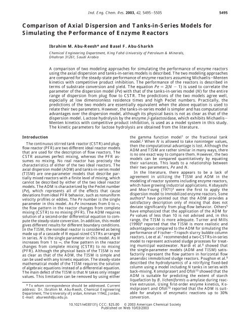
Figure 1 shows the conversions predicted by both the
ADM (Pe ≈ 0) and one-CSTR (N ) 1) model as a
function of the dimensionless residence time, θ; the
dimensionless Michaelis-Menten constant, K′ m ; and
the ratio of the Michaelis-Menten constant to inhibition
constant, . The Pe value used in Figure 1 is 0.0001 to
avoid division by zero in the ADM. Equation 31 [i.e., Pe

Figure 1. Conversion vs dimensionless residence time for N ) 1 and Pe ) 0.0001
) 2(N - 1)] is used to relate Pe and N. It is clear that
this equation represents the complete-mixing limit
correctly (i.e., Pe ) 0 and N ) 1). Three values of are
used in Figure 1 (0, 0.1, and 10). ) 0 corresponds to
Michaelis-Menten kinetics with no inhibition by the
product. Increasing the value of increases the product
inhibition. Three values of K′ m are also shown in the
figure (0.1, 1, and 10). From Figure 1, it is clear that
increasing θ increases the substrate conversion and
increasing K′ m reduces the conversion because the rate
of reaction decreases with increasing K′ m . At very low
values of K′ m (K′ m f 0), the enzyme kinetics approaches
zeroth-order, whereas at very high values of K′ m (K′ m f
∞), the enzyme kinetics approaches first-order. Also
from Figure 1, it can be seen that increasing the value
of reduces the conversion. This is expected because
the product inhibition reduces the rate of the enzymatic
reaction. It is clear from Figure 1 that both the ADM
and the TISM agree very well in predicting the enzyme
reactor conversion using eq 31 to relate the parameters
of the two models, Pe and N. Actually, the two models
are identical when Pe f 0 and N f 1. Equation 31
represents the perfect-mixing limit of the dispersion
range correctly and is simpler than eq 29. Equation 30
predicts Pe f 2 instead of Pe f 0 at complete mixing.
Figure 2a shows the substrate conversion predicted
from the ADM at Pe ) 2 and the TISM at N ) 2
according to eq 31 describing the relationship between
Pe and N. A conversion trend similar to that of Figure
1 is obtained. Comparing Figure 1 and Figure 2a shows
that increasing Pe increases the conversion. This is
expected for such an enzyme kinetic equation. Comparing
the values of conversion predicted by the two models
in Figure 2a shows that they agree well, especially at
low dimensionless residence times, θ (low Damkholer
numbers or slow reactions). Deviations occur only at
high dimensionless residence times (high conversions).
Using eq 29 to relate the parameters of the two
models (Pe and N), larger deviations were observed in
the predicted conversions of the two models than were
Ind. Eng. Chem. Res., Vol. 42, No. 22, 2003 5499
obtained using eq 31. Figure 2b shows the conversion
predicted by the TISM at N ) 2 and the ADM at Pe )
2.557 (according to eq 29). The deviation in conversion
is larger, especially at high dimensionless residence
times, although the simpler relation Pe ) 2(N - 1) gives
smaller errors than the variance-matching procedure for
large dimensionless residence times. There is no explanation
or justification for this observation. In Figure 2a
and b, it is clear that the ADM predicts higher conversions
than the TISM at high dimensionless residence
times.
Decreasing the intensity of mixing with increasing
values of N and Pe improved the agreement between
the two models. Figure 3 shows the conversions predicted
using the TISM with N ) 3 and the ADM with
Pe ) 4, according to eq 31. Similar results were obtained
for the case of N ) 5 and Pe ) 8, as shown in Figure 4.
As will be shown later, in the low-dispersion region
(high Pe), the higher the Pe, the higher the θ at which
the two models begin to diverge.
Figure 5 shows the predicted yields from both the
TISM with N ) 5 and the ADM with Pe ) 8 as a
function of the dimensionless residence time, θ; the
dimensionless Michaelis-Menten constant, K′ m ; and
the ratio of the Michaelis-Menten constant to the
inhibition constant, . It is clear from Figure 5 that the
yield decreases with increasing dimensionless residence
time, i.e., high yields are predicted for slow reactions
and visa versa. As given by eqs 27 and 28, the yield is
equal to the conversion divided by the dimensionless
residence time. The effect of K′ m on the yield is more
important in the case of slow reactions with no product
inhibition, as increasing the K′ m value decreases the
yield. At high ratio of the Michaelis-Menten constant
to the inhibition constant ( ) 10), the K′ m value has
little effect on the reactor yield, especially at high
dimensionless residence times (fast reactions). It is also
clear from Figure 5 that the yield decreases with
increasing , especially for low values of K′ m . Again, in
Figure 5, an excellent agreement is observed between

5500 Ind. Eng. Chem. Res., Vol. 42, No. 22, 2003
Figure 2. Conversion vs dimensionless residence time for N ) 2 and (a) Pe ) 2 and (b) Pe ) 2.557.
the yields predicted by the TISM (N ) 5) and the ADM
(Pe ) 8). This is expected because a high level of
agreement is obtained in the predicted conversions, as
shown in Figure 4, and the yield depends on the
conversion and the dimensionless residence time, as
given by eqs 27 and 28.
The conversion of milk (or whey) lactose to glucose
and galactose by the enzyme -galactosidase was studied
using the two modeling approaches as discussed
above in the case studies. Figure 6 describes the first
case study (K′ m ) 0.159 and ) 1.517), which corresponds
to lactose hydrolysis at a reactor temperature
of 40 °C. The x coordinate in Figure 6 is 1/Pe for the
ADM and 1/[2(N - 1)] for the TISM. The x coordinates
of the two models are equal if we use eq 31 to relate
the parameters of the two models. In Figure 6, the
symbols represent points for N ) 2-11 CSTRs in series,
whereas the continuous lines represent the results for
the ADM. From Figure 6, it is clear that conversion
increases with increasing dimensionless residence time
and decreases with increasing intensity of mixing. The
effect of the intensity of mixing is important only at high
values of the dimensionless residence time (fast reactions).
As shown in Figure 6, the conversions predicted

Figure 3. Conversion vs dimensionless residence time for N ) 3 and Pe ) 4.
Figure 4. Conversion vs dimensionless residence time for N ) 5 and Pe ) 8.
by the two models agree well, and deviations can be
observed only at high θ and high intensity of mixing
such as N ) 2.
For first-order reactions, both the ADM and the TISM
are easy to apply. When ) 1, the axial dispersion
model for Michaelis-Menten kinetics with competitive
product inhibition reduces to first-order kinetics with
the analytical solution given by eq 15. The second case
Ind. Eng. Chem. Res., Vol. 42, No. 22, 2003 5501
study ( ) 1, Km ) Ki ) 5.206 × 10 -4 mol/L) corresponds
to lactose hydrolysis at 7 °C. 24 Figure 7 shows the
conversions predicted by the ADM and TISM as a
function of dimensionless residence time for ) 1. The
N values shown in the figure are 1, 2, 3, and 5, and the
corresponding Pe numbers are 0, 2, 4, and 8, respectively,
according to eq. 31. The PFR conversion is also
shown in Figure 7 for comparison. The difference in the

5502 Ind. Eng. Chem. Res., Vol. 42, No. 22, 2003
Figure 5. Yield vs dimensionless residence time for N ) 5 and Pe ) 8.
Figure 6. Lactose conversion using dispersion and tanks-in-series
models at 40 °C (K′ m ) 0.159 and ) 1.517).
conversions predicted by the two models is very small.
For N ) 1 and Pe ) 0, the two models are equivalent.
The largest absolute difference in the conversions
predicted by the two models is 0.0125 for N ) 2 and Pe
) 2. This difference decreases with increasing N and
Pe. For N ) 3 and N ) 5, the largest absolute differences
in the predicted conversions between the two models
are 0.007 47 and 0.003 39, respectively.
For the case of ) 1, K′ m is very small (3.561 × 10 -3
mol/L). For K′ m , 1, eqs 38 and 39 are applied to our
kinetic equation. θ* is the dimensionless residence time
at which the exit concentrations of the two models differ
by at most a factor of e. To determine the range of θ at
which the predictions of the two models diverge, the
ratio of the exit substrate concentrations for the TISM
and ADM is plotted as a function of θ in Figure 8a for
Pe ) 100 and Pe ) 50. The corresponding values of θ*
(according to eq 38) are 24.8 and 15.6, respectively. At
low θ (θ < θ*, slow reactions), the predictions of the two
models agree very well. At high θ (θ > θ*, fast reactions),
the predictions of the two models diverge. In practice,
most conversion is achieved at θ < θ*. For example,
most commercial processes operate at lactose conversion
level of 80% or greater. 26 Figure 8b shows the same
comparisons between the two models but for Pe < 10.
For first-order kinetics ( ) 1) and ADM close to perfect
mixing, i.e., Pe f 0(N f 1), Dommeti and Balakotaiah 16
derived eq 39 which relates θ* and Pe in this mixing
region. From eq 39, it is clear that, as Pe f 0, the value
of θ* at which the two models begin to diverge becomes
very large. For example, in Figure 8b, when Pe ) 0.0001,
θ* ) 72 100 (from eq 39). This is very close to the case
of Pe ) 0 for the ADM and N ) 1 for the TISM, where
the two models are equivalent. It can be seen from
Figure 8a and b that the ADM and TISM agree very
well at low θ and high Pe. Divergence occurs only at
very high θ (high conversion) especially for low Pe. As
shown in Figure 8a and b, the ADM always predicts
higher conversions than the TISM at very high dimensionless
residence times. In the case of small dimensionless
residence times θ (low Da),the difference SN - SL
is third-order in θ for the variance-matching method (eq
29), 16 whereas this difference is quadratic in θ using the
equation Pe ) 2(N - 1). It should be clear that it makes
no sense to compare the exit concentrations of the two
models at very large θ (Da f ∞).
The predictions of the two models can be compared
for * 1 by using a numerical solution for the ADM
boundary value problem as shown above. For nonlinear
kinetics, such as Michaelis-Menten with competitive
product inhibition, the upper limit of θu for which the

Figure 7. Lactose conversion vs dimensionless residence time for ) 1 (temperature ) 7 °C) and initial lactose concentration ) 5wt%.
predictions of the two models agree is given by 16
where |f ′(SN)| is the absolute value of the first derivative
with respect to concentration of the normalized reaction
rate at the exit concentration. For θ < θ* (slow reactions),
the predictions of the two models agree well. For
θ > θ* (fast reactions), the predictions of the two models
diverge , and the TISM cannot be used to describe the
ADM.
Conclusions
θ u ) 1.15Pe2/3
|f ′(S N )|
θ u )
7.21
Pe|f ′(S N )|
for Pe f ∞ (Nf ∞) (40)
for Pe f 0(N f 1) (41)
Two modeling approaches based on the ADM and
TISM were developed for simulating the steady-state
performance of a reactor performing enzymatic reactions
described by Michaelis-Menten kinetics with competitive
product inhibition.
Ind. Eng. Chem. Res., Vol. 42, No. 22, 2003 5503
The equation Pe ) 2(N - 1) was found to describe
the relationship between Pe and N for the whole range
of dispersion between plug flow and complete mixing,
including the two limits Pe f 0(N f 1) and Pe f ∞ (N
f ∞). Using this equation, the conversions and yields
predicted by the two models were found to agree well,
especially at high Peclet numbers and low dimensionless
residence times.
Differences between the predictions of the two models
appear only at very high dimensionless residence times.
Simulation results showed that there is an upper bound
on the dimensionless residence time, θ*, at which the
predictions by the two models begin to diverge. This
upper bound on θ depends on Pe. In the low-dispersion
region, the higher Pe, the higher θ*. For the case of
infinite dispersion (Pe f 0, N f 1), the θ* value at which
the two models begin to diverge is very large. For Pe )
0 and N ) 1, the two models are identical. In general,
using the simple equation Pe ) 2(N - 1), the difference
between the conversions predicted by the two models
disappears for practical purposes. However, the tanksin-series
model presents computational advantages
compared to dispersion model.

5504 Ind. Eng. Chem. Res., Vol. 42, No. 22, 2003
Figure 8. Ratio of exit concentrations for the TISM and ADM as
a function of dimensionless residence time, ) 1, for (a) Pe ) 50,
100 and (b) Pe e 10.
For equal Michaelis-Menten and inhibition constants
( ) 1), the nonlinear Michaelis-Menten kinetics with
competitive product inhibition is reduced to first-order
kinetics, allowing the dispersion equation with Danckwerts
boundary conditions to be solved analytically. The
enzymatic conversion of lactose to glucose and galactose
is examined as a model system. Lactose conversion is
determined at the two temperatures of 40 and 7 °C.
Lactose hydrolysis is described by first-order kinetics
at7°C( ) 1), which allows the ADM to be solved
analytically.
Acknowledgment
The authors acknowledge the support provided by
King Fahd University of Petroleum & Minerals,-
Dhahran, Saudi Arabia.
Nomenclature
a, b, c ) parameters defined in eq 11
Dz ) axial dispersion coefficient (m 2 /h)
f(R) ) normalized reaction rate [f(1) ) 1]
g(θ,Pe) ) function defined in eq 34
Ki ) inhibition constant (mol/L)
Km ) Michaelis-Menten constant (mol/L)
K′m ) dimensionless Michaelis-Menten constant (Km/So)
L ) reactor length (m)
N ) number of mixed tanks in series
P ) product concentration (mol/L)
q ) parameter defined in eq 15
R(S,P) ) reaction rate (mol/L‚h)
S ) substrate concentration (mol/L)
t ) time (h)
T ) temperature (K)
u ) interstitial liquid velocity (m/h)
Vmax ) maximum reaction rate (mol/L‚h)
X ) substrate conversion
x ) dimensionless axial distance (Z/L)
Y ) yield
Z ) axial distance in the reactor (m)
Greek Letters
R)dimensionless substrate concentration (S/So)
) deviation parameter (defined in eq 37)
) dimensionless ratio of (Km/Ki)
τ ) residence time (h)
θ ) dimensionless residence time (Vmaxτ/So)
Dimensionless Numbers
Da ) Damkohler number (Vmaxτ/So)
Pe ) Peclet number (uL/Dz)
Subscripts and Superscripts
i ) refers to the ith reactor
L ) effluent
N ) refers to the Nth reactor
o ) initial
PFR ) plug-flow reactor
total ) total of all reactors
Z ) axial direction
* ) critical value for linear kinetics
u ) upper bound
Abbreviations
ADM ) axial dispersion model
CSTR ) continuous stirred tank reactor
PFR ) plug-flow reactor
TISM ) tanks-in-series model
Literature Cited
(1) Buffham, B. A.; Gibilaro, L. G. A generalization of the tanks
in series mixing model. AIChE J. 1968, 14, 805-806.
(2) Stokes, R. L.; Nauman, E. B. Residence time distribution
functions for stirred tanks in series. Can. J. Chem. Eng. 1970,
48, 723-725.
(3) Kobayashi, T.; Moo-Young, M. Backmixing and mass transfer
in the design of immobilized enzyme reactors. Biotechnol.
Bioeng. 1971, 13, 893-910.
(4) Wen, C. Y.; Fan, L. T. Models for Flow Systems and
Chemical Reactors; Marcel Dekker: New York, 1975.
(5) Shinnar, R. Use of residence and contact time distributions
in reactor design. In Chemical Reaction and Reactor Engineering;
Carberry, J., Varma, A., Eds.; Marcel Dekker: New York, 1987.
(6) Turner, J. R.; Mills, P. L. Comparison of axial dispersion
and mixing cell models for design and simulation of Fischer-
Tropsch slurry bubble column reactors. Chem. Eng. Sci. 1990, 45
(8), 2317-2324.
(7) Lee, T. T.; Wang, F. Y.; Newell, R. B. A generalized
procedure for modeling and simulation of activated sludge plant
using lumped-parameter approach. J. Environ. Sci. Health A 1997,
32 (1), 83-104.
(8) Nardi, I. R.; Zaiat, M.; Foresti, E. Influence of the tracer
characteristics on hydrodynamic models of packed bed reactors.
Bioprocess Eng. 1999, 21 (5), 469-476.

(9) Poughon, L.; Dussap, C. G.; Gros, J. B. Dynamic model of a
nitrifying fixed bed column: Simulation of the biomass distribution
of Nitrosomonas and Nitrobacter and of transient behavior of the
column. Bioprocess Eng. 1998, 20 (3), 209-221.
(10) Komolprasert, V.; Ofoli, R. Y. A dispersion model for
predicting the extent of starch liquefaction by B. licheniformis
R-amylase during reactive extrusion. Biotechnol. Bioeng. 1991, 37,
681-690.
(11) Elgeti, K. A new equation for correlating a pipe flow reactor
with a cascade of mixed reactors. Chem. Eng. Sci. 1996, 51, 5077-
5080.
(12) Kramers, H.; Alberda, G. Frequency response analysis of
continuous flow systems. Chem. Eng. Sci. 1953, 2, 173-181.
(13) Aris, R. End and beginnings in the mathematical modeling
of chemical engineering systems. Chem. Eng. Sci. 1993, 48 (14),
2507-2517.
(14) Van Hasselt, B. W.; Calis, H. P. A.; Sie, S. T.; Van den
Bleek, C. M. Gas- and liquid-phase residence time distribution in
the three levels of porosity reactor. Chem. Eng. Sci. 1999, 54,
5047-5053.
(15) Ponzi, E. N.; Gonzalez, M. G. Comparison between the
dispersion and tanks in series models. Chem. Eng. Sci. 1980, 35
(8), 1804-1806.
(16) Dommeti, S. M. S.; Balakotaiah, V. On the limits of validity
of effective dispersion models for bulk reactions. Chem. Eng. Sci.
2000, 55, 6169-6186.
(17) Fogler, H. S. Elements of Chemical Reaction Engineering,
3rd ed.; Prentice Hall: Upper Saddle River, NJ, 1999.
(18) Danckwerts, P. V. Continuous flow systems, Distribution
of residence times. Chem. Eng. Sci. 1953, 2 (1), 1-18.
Ind. Eng. Chem. Res., Vol. 42, No. 22, 2003 5505
(19) Nauman, E. B. Chemical Reactor Design; John Wiley and
Sons: New York, 1987.
(20) IMSL Software, Visual Numerics, Inc.: Houston, TX, 1987
(support@imsl.com).
(21) Lortie, R. Evaluation of the performance of immobilized
enzyme reactors with Michaelis-Menten kinetics. J. Chem. Technol.
Biotechnol. 1994, 60, 189-193.
(22) Abu-Reesh, I. M. Predicting the performance of immobilized
enzyme reactors using reversible Michaelis-Menten kinetics.
Bioprocess Eng. 1997, 17 (3) 131-137.
(23) Balakotaiah, V. Some comments on “A new equation for
correlation of a pipe flow reactor with a cascade of mixed reactors”.
Chem. Eng. Sci. 1998, 53 (9), 1787.
(24) Santos, A.; Ladero, M.; Garcia-Ochoa, F. Kinetic modeling
of lactose hydrolysis by -galactosidase from Kluyveromices fragillis.
Enzyme Microb. Technol. 1998, 22, 558-567.
(25) Abu-Reesh, I. M. Optimal design for CSTRs in series
performing enzymatic lactose hydrolysis. Bioprocess Eng. 2000,
23 (6), 709-713.
(26) Yang, S. T.; Okos, M. R. Effects of temperature on lactose
hydrolysis by immobilized -galactosidase in plug-flow reactor.
Biotechnol. Bioeng. 1989, 33, 873-885.
Received for review February 12, 2003
Revised manuscript received July 25, 2003
Accepted August 19, 2003
IE030131J