simulation of offgas scrubbing by a combined eulerian ... - CFD

The force balance for a single dust particle can be written
as
2
ρ Pu
Drift 24
mPu&
P = mP
g − A .
P
2 Re
Using the particle relaxation time,
Copyright © 2009 CSIRO Australia 4
τ
P
ρ d
2
P P
P,
relax = ,
18μG
above equation can be written as
u& u Drift
= g − . (7)
P
τ
P,
relax
Assuming local equilibrium one can assume that:
∂uG
u& P = + ( ∇ ⋅u
G ) u (8)
G
∂t
Thus, using equations (7) and (8) the drift velocity can be
calculated from the gas velocity and the particle
properties.
The dispersion of particles strongly depends on the
turbulence structure. According to Crowe (1985), the
reciprocal Schmidt number denoting the ratio of
diffusivity and effective viscosity is a function of the time
τ τ ,
ratio P , relax G,
turb
Ddiff
ρG
⎛τ
⎞ P,
relax
= F⎜
⎟ . (9)
η ⎜ ⎟
G ⎝ τ G,
turb ⎠
Hereby, in RANS simulations using the k-ε turbulence
model the characteristic time of large scale turbulent
structures can be approximated as
τ
k
0.
15
ε
G,
turb = . (10)
Thus, using above correlation the dust phases diffusivity
can be calculated from turbulence parameters and the dust
particles’ relaxation time.
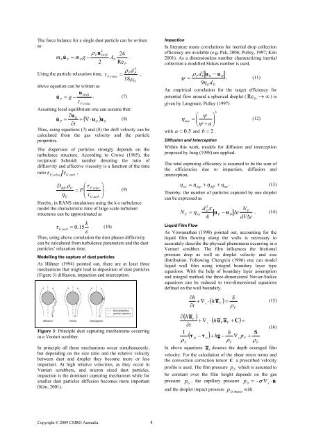
Modelling the capture of dust particles
As Hähner (1994) pointed out, there are at least three
mechanisms that might lead to deposition of dust particles
(Figure 3) diffusion, impaction and interception.
Figure 3: Principle dust capturing mechanisms occurring
in a Venturi scrubber.
In principle all these mechanisms occur simultaneously,
but depending on the size ratio and the relative velocity
between dust and droplet they become more or less
important. At high relative velocities, as they occur in
Venturi scrubbers, and micron sized dust particles,
impaction is the dominant capturing mechanism while for
smaller dust particles diffusion becomes more important
(Kim, 2001).
Impaction
In literature many correlations for inertial drop collection
efficiency are available (e.g. Pak, 2006; Pulley, 1997; Kim
2001). As a dimensionless number characterizing inertial
collection a modified Stokes number is used,
ψ
ρ d
u − u
=
P
2
P G
9η
Gd
D
D
. (11)
An empirical correlation for the target efficiency for
potential flow around a spherical droplet ( Re D → ∞ ) is
given by Langmuir, Pulley (1997)
imp
a ⎟ ⎛ ψ ⎞
η = ⎜
⎝ψ
+ ⎠
with a = 0.
5 and b = 2 .
(12)
Diffusion and Interception
b
Within this work, models for diffusion and interception
proposed by Jung (1998) are applied.
The total capturing efficiency is assumed to be the sum of
the efficiencies due to impaction, diffusion and
interception,
η +
= η + η η . (13)
tot imp diff int
Thereby, the number of particles captured by one droplet
can be expressed as
N
C
Liquid Film Flow
2
d Dπ
N P
= η tot u P − u D Δt
. (14)
4
dVΔt
As Viswanathan (1998) pointed out, accounting for the
liquid film flowing along the walls is necessary to
accurately describe the physical phenomena occurring in a
Venturi scrubber. The film influences the frictional
pressure drop as well as droplet velocity and size
distribution. Following Chengxin (1996) one can model
liquid wall film using integral boundary layer type
equations. With the help of boundary layer assumption
and integral method, the three-dimensional Navier-Stokes
equations can be reduced to two-dimensional equations
defined on the wall boundary.
∂h
+ ∇
∂t
( hu
)
∂
∂t
1
ρ
F
F
s
⋅
( τ − τ )
fs
+ ∇
w
s
S
u F =
(15)
ρ
( h )
⋅
F
( hu
u + C)
F
F
h
+ hg
− ∇
ρ
F
s
=
p
F
S
+
ρ
F
(16)
In above equations u denotes the depth averaged film
F
velocity. For the calculation of the shear stress terms and
the convection correction tensor C a prescribed velocity
profile is used. The film pressure p which is assumed to
F
be constant over the film height depends on the gas
p , the capillary pressure n ⋅ ∇ − p σ
pressure G
and the droplet impact pressure p with
D,
impact
= σ
s