proceedings - International Tissue Elasticity Conference

011 SIMULATION OF 3D STRAIN IMAGING USING 2D ARRAY TRANSDUCERS.
M Rao 1 , T Varghese 1 , JA Zagzebski 1 .
University of Wisconsin–Madison, 1530 Medical Sciences Center, 1300 University Avenue,
Madison, WI 53706, USA.
Background: Displacement vector and strain tensor imaging in three dimensions requires acquisition of
3D volume data in real time. Two–dimensional (2D) transducer arrays represent a promising solution for
implementing real time 3D data acquisition. Previously, we described a frequency domain B–mode
imaging model applicable for linear and phased array transducers [1]. In this study, we extend this model
to incorporate 2D array transducers and apply it to simulate 3D strain imaging.
Aims: The aim of this study is to extend a frequency domain ultrasound simulation model to 2D array
transducers and to utilize the model to generate simulated 3D strain images.
Methods: The pressure field for a 64×64 square array with element dimensions of 0.15 mm and
center–to–center spacing of 0.2 mm was calculated by applying the paraxial approximation to solve
the 2D Rayleigh integral for each element. We assume a rigid baffle, no apodization, a 5 MHz center
frequency, and a speed of sound of 1540 m/s. A single transmit focus at 30 mm and dynamic receive
focus with an F–number of 2 was utilized. The 2D array model was compared with the widely used
ultrasound simulation program FIELD II, which utilizes an approximate form of the time domain
impulse response function. For strain imaging, we incorporate frame–to–frame displacements using
Finite Element Analysis (FEA) simulation using ANSYS software (ANSYS Inc., Canonsburg, USA). 1D,
2D and 3D motion tracking algorithms for tracking displacement vectors were compared.
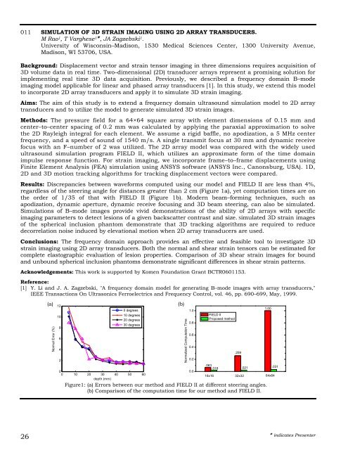
Results: Discrepancies between waveforms computed using our model and FIELD II are less than 4%,
regardless of the steering angle for distances greater than 2 cm (Figure 1a), yet computation times are on
the order of 1/35 of that with FIELD II (Figure 1b). Modern beam–forming techniques, such as
apodization, dynamic aperture, dynamic receive focusing and 3D beam steering, can also be simulated.
Simulations of B–mode images provide vivid demonstrations of the ability of 2D arrays with specific
imaging parameters to detect lesions of a given backscatter contrast and size. Simulated 3D strain images
of the spherical inclusion phantom demonstrate that 3D tracking algorithms are required to reduce
decorrelation noise induced by elevational motion when 2D array transducers are used.
Conclusions: The frequency domain approach provides an effective and feasible tool to investigate 3D
strain imaging using 2D array transducers. Both the normal and shear strain tensors can be estimated for
complete elastographic evaluation of lesion properties. Comparison of 3D shear strain images for bound
and unbound spherical inclusion phantoms demonstrate significant differences in shear strain patterns.
Acknowledgements: This work is supported by Komen Foundation Grant BCTR0601153.
Reference:
[1] Y. Li and J. A. Zagzebski, "A frequency domain model for generating B–mode images with array transducers,"
IEEE Transactions On Ultrasonics Ferroelectrics and Frequency Control, vol. 46, pp. 690–699, May, 1999.
26
(a) (b)
Normal Error (%)
12
10
8
6
4
2
0 degrees
10 degrees
20 degrees
30 degrees
0
0 10 20 30
depth (mm)
40 50 60
Normalized Computation Time
1.0
0.8
0.6
0.4
0.2
0.0
FIELD II
Proposed method
.063
.018
Figure1: (a) Errors between our method and FIELD II at different steering angles.
(b) Comparison of the computation time for our method and FIELD II.
16x16
.259
32x32
.021
1.00
64x64
.031
indicates Presenter