download vol 5, no 3&4, year 2012 - IARIA Journals

International Journal on Advances in Telecommunications, vol 5 no 3 & 4, year 2012, http://www.iariajournals.org/telecommunications/
where
2
K
i=1 k=1
j ∈ Ω ⇔
bi,k,spi,k
j q(j − Bi,k) = jsq(j) (10)
j1 ≤ C1 ∩
2
s=1
js ≤ C2
(11)
The parameter s refers to the systems (s = 1 indicates the
active system, s = 2 the passive system), while i refers to
the states (i = 1 specifies the active state, i = 2 specifies the
passive state). Also,
bk, if s = i
bi,k,s =
(12)
0, if s = i
and Bi,k = (bi,k,1, bi,k,2) is the i,k row of the (2K×2) matrix
B, with elements bi,k,s. Also, pi,k(j) is the utilization of the
i-th system by service-class k:
pi,k
j =
λk[1−lbk(j1−bk)]
(1−vk)µ1k
λkvk
(1−vk)µ2k
for i = 1
for i = 2
Moreover, js is the occupied capacity of the system:
js =
2
K
i=1 k=1
n i kbi,k,s
(13)
(14)
Proof: In order to derive the recursive formula of (10) we
introduce the following notation:
n = (n 1 , n 2 ), n i = (n i 1, n i 2, ..., n i K ),
n i k+ = (ni 1, ..., n i k + 1, ..., ni K ),
n i k− = (ni 1, ..., n i k − 1, ..., ni K ),
n 1 k+ = (n1 k+ , n2 ), n 2 k+ = (n1 , n 2 k+ ),
n 1 k− = (n1 k− , n2 ), n 2 k− = (n1 , n 2 k− )
(15)
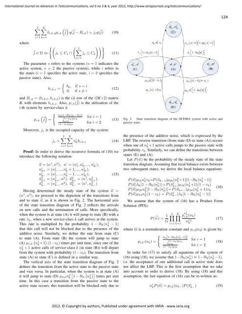
Having determined the steady state of the system n =
(n 1 , n 2 ), we proceed to the depiction of the transitions from
and to state n, as it is shown in Fig. 2. The horizontal axis
of the state transition diagram of Fig. 2 reflects the arrivals
on new calls and the termination of calls. More specifically,
when the system is at state (A) it will jump to state (B) with a
Fig. 2. State transition diagram of the OCDMA system with active and
passive users.
the presence of the additive noise, which is expressed by the
LBP. The reverse transition (from state (D) to state (A)) occurs
when one of n1 k +1 active calls jumps to the passive state with
probability vk. Similarly, we can define the transitions between
states (E) and (A).
Let P (n) be the probability of the steady state of the state
transition diagram. Assuming that local balance exists between
two subsequent states, we derive the local balance equations:
P (n)µikn1 kvk=P (nk−+)µ2k(n 2 k +1)[1−lbk(n 1 k−1)] P (n)λk[1 − lbk(n1 k )]=P (n1 k+ )µ1k(n1 k +1)(1 − vk)
P (n)µ2kn 2 k [1 − lbk(n1 k )]=P (nk+−)µ1k(n1 k + 1)vk
P (n)µ1kn 1 k (1 − vk) = P (n 1 k− )λk[1 − lbk(n1 k − 1)]
rate λk, when a new service-class k call arrives at the system.
This rate is multiplied by the probability 1 − lbk(n1 k − 1)
that this call will not be blocked due to the presence of the
additive noise. Similarly, we define the rate from state (C)
to state (A). From state (B) the system will jump to state
1 (A) µ1,k nk +1 (1−vk) times per unit time, since one of the
n1 k + 1 active calls of service-class k (in state (B)) will depart
from the system with probability (1 − vk). The transition from
state (A) to state (C) is defined in a similar way.
The vertical axis of the state transition diagram of Fig. 2
defines the transition from the active state to the passive state
and vice versa. In particular, when the system is at state (A)
it will jump to state (D) µ2,kn2 P (
1
k 1 − lbk nk times per unit
time. In this case a transition from the passive state to the
active state occurs; this transition will be blocked only due to
⇀ n) = 1
2 K p
G
i=1 k=1
n1
k
i,k (nk)
n1 k !
(17)
where G is a normalization constant and pi,k(nk) is given by:
λk[1−lbk(n
pi,k (nk) =
1
k−1)] for i = 1
(1−vk)µ1k
(18)
λkvk for i = 2
(1−vk)µ2k
In order for (17) to satisfy all equations of the system of
(16) using (18), we assume that 1−lbk(n 1 k ) ≈ 1−lbk(n 1 k −1),
i.e. the acceptance of one additional call in active state does
not affect the LBP. This is the first assumption that we take
into account in order to derive (10). By using (18) and this
assumption, the last equation of (16) can be re-written as:
n i kP (n) = pi,k(nk−)P (n i k−) (19)
2012, © Copyright by authors, Published under agreement with IARIA - www.iaria.org
(16)
We assume that the system of (16) has a Product Form
Solution (PFS):
124