download vol 5, no 3&4, year 2012 - IARIA Journals
download vol 5, no 3&4, year 2012 - IARIA Journals
download vol 5, no 3&4, year 2012 - IARIA Journals

You also want an ePaper? Increase the reach of your titles
YUMPU automatically turns print PDFs into web optimized ePapers that Google loves.
International Journal on Advances in Telecommunications, <strong>vol</strong> 5 <strong>no</strong> 3 & 4, <strong>year</strong> <strong>2012</strong>, http://www.iariajournals.org/telecommunications/<br />
IV. SYSTEM MODEL OF A MULTI-RATE OCDMA PON<br />
WITH QOS GUARANTEES<br />
In OCDMA networks, QoS differentiation can be realised<br />
by the utilization of codewords with different weights. To this<br />
end, we assume that the PON supports K = T · F serviceclasses:<br />
F service-classes are differentiated by the data rate,<br />
while each one of these F service-classes supports T different<br />
QoS levels that express different values of the BER at the<br />
receiver. We also consider that the PON assigns (L, Wt, λa, 1)<br />
codewords to service-class t, t = 1, ..., T . Calls of these T<br />
service-classes require the same number bf,t (f = 1, ..., F )<br />
of codewords, while they are differentiated by the weight<br />
Wt. The received power per bit “1” of service-class f, t is<br />
de<strong>no</strong>ted as I f,t<br />
unit , while the received power that corresponds<br />
to a call of service-class f, t is at most Iact f,t = bf,t · I f,t<br />
unit .<br />
The traffic parameters of service-class f, t are de<strong>no</strong>ted as<br />
(λf,t, µ −1<br />
1,f,t , µ−1<br />
2,f,t , vf,t). To simplify the presentation of these<br />
parameters we use one <strong>no</strong>tation for the service-classes; we<br />
de<strong>no</strong>te that the parameters of service-class k (k = 1, . . . , T ·F )<br />
are I k unit<br />
= If,t<br />
unit , Ik act = I f,t<br />
act, bk = bf,t, λk = λf,t,<br />
µ −1<br />
ik = µ−1<br />
i,f,t and vk = vf,t.<br />
In order to determine the LBP of service-class k, we use<br />
the following relation, which is based on (6):<br />
lbk(n 1 k )=P<br />
1−lbk(n 1 k )=P<br />
IN<br />
Imax<br />
IN<br />
Imax<br />
·F<br />
>1−T<br />
x=1<br />
<br />
·F<br />
≤1−T<br />
x=1<br />
n1 bx·I<br />
x<br />
x<br />
unit<br />
Imax<br />
<br />
n 1 k<br />
bx·I x<br />
unit<br />
Imax<br />
<br />
x,k<br />
Pinterf where the probability of interference P x,k<br />
P x,k<br />
interf<br />
− Ik<br />
<br />
act ⇔ Imax<br />
<br />
− Ik<br />
<br />
act<br />
Imax<br />
(33)<br />
between two<br />
interf<br />
codewords with weights Wx and Wk is a function of the hit<br />
probability [26]:<br />
px,k = WxWk<br />
2L<br />
(34)<br />
The probability of interference of a codeword of a serviceclass<br />
k assigned to a new arriving call and a codeword<br />
of service-class x can be calculated by following the same<br />
procedure that was used in order to derive (3):<br />
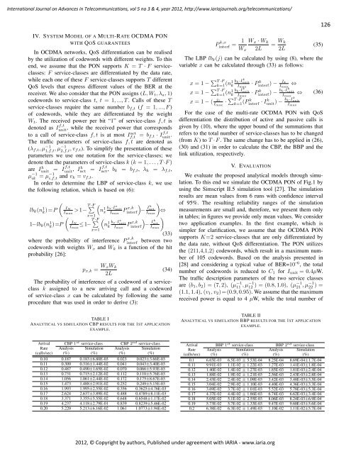
TABLE I<br />
ANALYTICAL VS SIMULATION CBP RESULTS FOR THE 1ST APPLICATION<br />
EXAMPLE.<br />
Arrival CBP 1 st service-class CBP 2 nd service-class<br />
Rate Analysis Simulation Analysis Simulation<br />
(calls/sec) (%) (%) (%) (%)<br />
0.10 0.187 0.183±6.80E-03 0.023 0.023±3.66E-03<br />
0.11 0.309 0.316±1.44E-02 0.041 0.043±3.40E-03<br />
0.12 0.487 0.490±1.65E-02 0.070 0.066±5.93E-03<br />
0.13 0.731 0.715±2.12E-02 0.112 0.110±5.76E-03<br />
0.14 1.056 1.061±2.44E-02 0.172 0.175±8.67E-03<br />
0.15 1.473 1.488±2.91E-02 0.252 0.249±5.15E-03<br />
0.16 1.993 1.995±2.55E-02 0.356 0.3625±4.76E-03<br />
0.17 2.624 2.637±3.89E-02 0.488 0.4789±8.11E-03<br />
0.18 3.371 3.355±5.55E-02 0.648 0.6548±1.17E-02<br />
0.19 4.237 4.118±2.79E-01 0.839 0.8239±5.46E-02<br />
0.20 5.220 5.213±6.16E-02 1.061 1.0773±1.94E-02<br />
P k,x 1 Wx · Wk<br />
interf =<br />
Wx 2L<br />
<strong>2012</strong>, © Copyright by authors, Published under agreement with <strong>IARIA</strong> - www.iaria.org<br />
= Wk<br />
2L<br />
(35)<br />
The LBP lbk(j) can be calculated by using (8), where the<br />
variable x can be calculated through (33) as follows:<br />
x = 1 − T ·F<br />
k=1 (n1 k<br />
x = 1 − T ·F<br />
k=1 (n1 k<br />
bk·I k<br />
unit<br />
Imax<br />
bk·I k<br />
unit<br />
Imax<br />
x = 1 − ( j1<br />
Imax · T ·F<br />
k=1<br />
· P k<br />
Ik<br />
interf ) − Imax ⇔<br />
· P k<br />
interf<br />
) − bk·I k<br />
unit<br />
Imax ⇔<br />
k (Pinterf · Ik k<br />
bk·Iunit unit ) − Imax<br />
(36)<br />
For the case of the multi-rate OCDMA PON with QoS<br />
differentiation the distribution of active and passive calls is<br />
given by (10), where the upper bound of the summations that<br />
refers to the total number of service-classes has to be changed<br />
(from K) to T ·F . The same change has to be applied in (26),<br />
(30) and (31) in order to calculate the CBP, the BBP and the<br />
link utilization, respectively.<br />
V. EVALUATION<br />
We evaluate the proposed analytical models through simulation.<br />
To this end we simulate the OCDMA PON of Fig.1 by<br />
using the Simscript II.5 simulation tool [27]. The simulation<br />
results are mean values from 6 runs with confidence interval<br />
of 95%. The resulting reliability ranges of the simulation<br />
measurements are small and, therefore, we present them only<br />
in tables; in figures we provide only mean values. We consider<br />
two application examples. In the first example, which is<br />
simpler for clarification, we assume that the OCDMA PON<br />
supports K=2 service-classes that are only differentiated by<br />
the data rate, without QoS differentiation. The PON utilizes<br />
the (211,4,1,2) codewords, which result in a maximum number<br />
of 105 codewords. Based on the analysis presented in<br />
[28] and considering a typical value of BER=10−6 , the total<br />
number of codewords is reduced to C1 for Iunit = 0.4µW.<br />
The traffic description parameters of the two service classes<br />
are (b1, b2) = (7, 2), (µ −1<br />
11 , µ−1 12 ) = (0.8, 1.0), (µ−1 21 , µ−1 22 ) =<br />
(1.1, 1.4), (v1, v2)=(0.9, 0.95). We assume that the maximum<br />
received power is equal to 4 µW, while the total number of<br />
TABLE II<br />
ANALYTICAL VS SIMULATION BBP RESULTS FOR THE 1ST APPLICATION<br />
EXAMPLE.<br />
Arrival BBP 1 st service-class BBP 2 nd service-class<br />
Rate Analysis Simulation Analysis Simulation<br />
(calls/sec) (%) (%) (%) (%)<br />
0.1 6.65E-03 6.5E-03 ± 5.53E-04 8.25E-04 8.69E-04±1.7E-04<br />
0.11 9.91E-03 1.1E-02 ± 1.22E-03 1.27E-03 1.41E-03±1.8E-04<br />
0.12 1.40E-02 1.4E-02 ± 1.27E-03 1.85E-03 1.81E-03±2.4E-04<br />
0.13 1.88E-02 1.9E-02 ± 1.21E-03 2.56E-03 2.43E-03±2.8E-04<br />
0.14 2.43E-02 2.4E-02 ± 1.09E-03 3.42E-03 3.48E-03±3.5E-04<br />
0.15 3.04E-02 2.9E-02 ± 1.10E-03 4.40E-03 4.36E-03±3.3E-04<br />
0.16 3.69E-02 3.7E-02 ± 1.01E-03 5.52E-03 5.78E-03±5.3E-04<br />
0.17 4.37E-02 4.4E-02 ± 1.86E-03 6.74E-03 6.62E-03±3.4E-04<br />
0.18 5.05E-02 5.1E-02 ± 2.55E-03 8.06E-03 8.24E-03±6.9E-04<br />
0.19 5.73E-02 5.7E-02 ± 1.33E-03 9.47E-03 9.60E-03±5.6E-04<br />
0.2 6.38E-02 6.3E-02 ± 1.49E-03 1.10E-02 1.11E-02±5.7E-04<br />
126