Using TIKZ - College of the Redwoods

Using TIKZ
David Arnold
College of the Redwoods
Department of Mathematics
November 20, 2010
David Arnold (CR) Using TIKZ November 20, 2010 1 / 24

Using Tikz
Open the file WorkshopFiles/workshop8.tex in TeXShop. Note the
new line \usepackage{tikz}, which loads the tikz package.
\ d o c u m e n t c l a s s { a r t i c l e }
\ usepackage [ n o s o l u t i o n s , p o i n t s o n l e f t ] { eqexam}
\ usepackage {amsmath}
\usepackage{tikz}
\ t i t l e {Exam \#2A}
\ s u b j e c t {Math 120}
\ a u t h o r { David Arnold }
\ date {November 20 , 2010}
Note also the new title and subject.
David Arnold (CR) Using TIKZ November 20, 2010 2 / 24

Exam Environment plus Instructions
There is a new exam environment and instructions. Compile.
\ b e g i n { document }
\ m a k e t i t l e
\ b e g i n {exam}{Exam2A}
\ b e g i n { i n s t r u c t i o n s }
Place the s o l u t i o n to each problem i n the space
p r o v i d e d .
\ end { i n s t r u c t i o n s }
\ end {exam}
\ end { document }
David Arnold (CR) Using TIKZ November 20, 2010 3 / 24

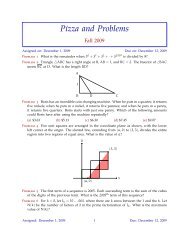
Create a Problem Environment
After the instructions environment, create a new problem environment.
Include a solution environment, reserving 3 inches of space for the user.
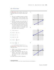
\ b e g i n { problem } [ 1 0 ] On the g r i d t h a t f o l l o w s , s k e t c h
the graph o f $y=2x +1$.
\ b e g i n { s o l u t i o n } [ 3 i n ]
S o l u t i o n h e r e .
\ end { s o l u t i o n }
\ end { problem }
After you enter the problem and solution code, recompile workshop8.tex.
David Arnold (CR) Using TIKZ November 20, 2010 4 / 24

Create a Grid
After the problem statement (and before the solution environment), enter
the grid code.
\ b e g i n { c e n t e r }
\ b e g i n { t i k z p i c t u r e }
\ draw [ gray ] (−5,−5) g r i d ( 5 , 5 ) ;
\ draw[, l i n e width=1pt ] ( −5 ,0) −−(5,0) node [ r i g h t
] { $ x $ } ;
\ draw[, l i n e width=1pt ] (0 , −5) −−(0,5) node [ above
] { $ y $ } ;
\ end { t i k z p i c t u r e }
\ end { c e n t e r }
After entering the grid code, recompile workshop8.tex.
David Arnold (CR) Using TIKZ November 20, 2010 5 / 24

Scaling the Grid
You can scale the grid as follows.
\ b e g i n { c e n t e r }
\ b e g i n { t i k z p i c t u r e } [ scale=0.5 ]
\ draw [ gray ] (−5,−5) g r i d ( 5 , 5 ) ;
\ draw[, l i n e width=1pt ] ( −5 ,0) −−(5,0) node [ r i g h t
] { $ x $ } ;
\ draw[, l i n e width=1pt ] (0 , −5) −−(0,5) node [ above
] { $ y $ } ;
\ end { t i k z p i c t u r e }
\ end { c e n t e r }
After you enter the scaling adjustment, recompile workshop8.tex.
David Arnold (CR) Using TIKZ November 20, 2010 6 / 24

Crafting a Solution
Copy the grid code into the solution environment.
\ b e g i n { s o l u t i o n } [ 3 i n ]
\ b e g i n { c e n t e r }
\ b e g i n { t i k z p i c t u r e } [ scale=0.5 ]
\ draw [ gray ] (−5,−5) g r i d ( 5 , 5 ) ;
\ draw[, l i n e width=1pt ] ( −5 ,0) −−(5,0) node [ r i g h t
] { $ x $ } ;
\ draw[, l i n e width=1pt ] (0 , −5) −−(0,5) node [ above
] { $ y $ } ;
\ end { t i k z p i c t u r e }
\ end { c e n t e r }
\ end { s o l u t i o n }
David Arnold (CR) Using TIKZ November 20, 2010 7 / 24

Drawing the Solution Line
We want to draw the graph of the line y = 2x + 1 on the grid. Use the
\draw command to do this. Add this single line immediately after the code
that creates the grid and just before the \end{tikzpicture} command.
\ draw[, l i n e width=1pt , b l u e ] (−3,−5) −−(2,5) node [
above r i g h t ] { $ y=2x +1$};
\ end { t i k z p i c t u r e }
After you enter the code to draw the graph of the line y = 2x + 1,
recompile workshop8.tex. Nothing happens because we haven’t yet
added the solutionsafter option.
David Arnold (CR) Using TIKZ November 20, 2010 8 / 24

Change the Preamble
To see solutions, use the option solutionsafter in the preamble.
\ d o c u m e n t c l a s s { a r t i c l e }
% Uncomment to p r o h i b i t s o l u t i o n s and p r o v i d e space
% f o r s t u d e n t work
% \ usepackage [ n o s o l u t i o n s , p o i n t s o n l e f t ] { eqexam}
% Uncomment to p r o v i d e s o l u t i o n s
\ usepackage [ s o l u t i o n s a f t e r , p o i n t s o n l e f t ] { eqexam}
Recompile workshop8.tex. The solution is now visible.
David Arnold (CR) Using TIKZ November 20, 2010 9 / 24

The Workarea
Open Workshopfiles/workshop9.tex in TeXShop. We moved the grid
code after problem statement into a workarea environment.
\ b e g i n { workarea }{\ sameVspace }
\ b e g i n { c e n t e r }
\ b e g i n { t i k z p i c t u r e } [ s c a l e =0.5]
\ draw [ gray ] (−5,−5) g r i d ( 5 , 5 ) ;
\ draw[, l i n e width=1pt ] ( −5 ,0) −−(5,0) node [ r i g h t
] { $ x $ } ;
\ draw[, l i n e width=1pt ] (0 , −5) −−(0,5) node [ above
] { $ y $ } ;
\ end { t i k z p i c t u r e }
\ end { c e n t e r }
\ end { workarea }
David Arnold (CR) Using TIKZ November 20, 2010 10 / 24

Solutions After versus No Solutions
Compile workshop9.tex with:
\ usepackage [ n o s o l u t i o n s , p o i n t s o n l e f t ] { eqexam}
In this case, the grid in the workarea environment will be
superimposed on the white space provided for student work.
Compile workshop9.tex with:
\ usepackage [ s o l u t i o n s a f t e r , p o i n t s o n l e f t ] { eqexam}
In this case, the workarea (whitespace for student work) is suppressed
and only the solution appears.
David Arnold (CR) Using TIKZ November 20, 2010 11 / 24

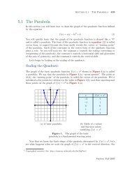
Plotting Functions
We’re now going to plot the graph of the function f (x) = x(x + 2)(x − 2).
Open WorkshopFiles/workshop10.tex in TeXShop and compile.
\ d o c u m e n t c l a s s { a r t i c l e }
\ usepackage { t i k z }
\ b e g i n { document }
\ b e g i n { t i k z p i c t u r e }
\ draw [ h e l p l i n e s ] (−5,−5) g r i d ( 5 , 5 ) ;
\ draw [ t h i c k ,] ( −5 ,0) −−(5,0) node [ r i g h t ] {$ x $ } ;
\ draw [ t h i c k ,] (0 , −5) −−(0,5) node [ above ] {$ y $ } ;
\ draw [ t h i c k , b l u e ] p l o t (\ x , { \ x ∗(\ x+2) ∗(\ x −2) }) ;
\ end { t i k z p i c t u r e }
\ end { document }
David Arnold (CR) Using TIKZ November 20, 2010 12 / 24

Restricting the Domain
You can restrict the domain of the function by adding the option
domain=-3:3.
\ b e g i n { t i k z p i c t u r e }
\ draw [ h e l p l i n e s ] (−5,−5) g r i d ( 5 , 5 ) ;
\ draw [ t h i c k ,] ( −5 ,0) −−(5,0) node [ r i g h t ] {$ x $ } ;
\ draw [ t h i c k ,] (0 , −5) −−(0,5) node [ above ] {$ y $ } ;
\ draw [ t h i c k , blue , domain=-3:3 ] p l o t (\ x , { \ x ∗(\ x+2) ∗(\ x
−2) }) ;
\ end { t i k z p i c t u r e }
Recompile workshop10.tex and note the difference.
David Arnold (CR) Using TIKZ November 20, 2010 13 / 24

Using Matlab to Restrict the Domain
You can your calculator or a software program such as MATLAB to
restrict the domain so that the range is restricted to [−5, 5].
syms x
f=x ∗( x+2) ∗( x −2) ;
s o l=s o l v e ( f −5,x ) ;
double ( s o l )
s o l=s o l v e ( f +5,x ) ;
double ( s o l )
ans =
2.4567
ans =
−2.4567
David Arnold (CR) Using TIKZ November 20, 2010 14 / 24

The Ideal Domain
Use the results from MATLAB to set domain=-2.4567:2.4567.
\ b e g i n { t i k z p i c t u r e }
\ draw [ h e l p l i n e s ] (−5,−5) g r i d ( 5 , 5 ) ;
\ draw [ t h i c k ,] ( −5 ,0) −−(5,0) node [ r i g h t ] {$ x $ } ;
\ draw [ t h i c k ,] (0 , −5) −−(0,5) node [ above ] {$ y $ } ;
\ draw [ t h i c k , blue , domain=-2.4567:2.4567 ] p l o t (\ x , { \ x ∗(\
x+2) ∗(\ x −2) }) ;
\ end { t i k z p i c t u r e }
Recompile workshop10.tex and note the difference.
David Arnold (CR) Using TIKZ November 20, 2010 15 / 24

Clipping Rectangle
A much simpler solution is to establish a clipping region. Use the scope
environment so that the clipping region affects only the graph of the
polynomial.
\ b e g i n { t i k z p i c t u r e }
\ draw [ h e l p l i n e s ] (−5,−5) g r i d ( 5 , 5 ) ;
\ draw [ t h i c k ,] ( −5 ,0) −−(5,0) node [ r i g h t ] {$ x $ } ;
\ draw [ t h i c k ,] (0 , −5) −−(0,5) node [ above ] {$ y $ } ;
\ b e g i n { scope }
\ c l i p (−5,−5) r e c t a n g l e ( 5 , 5 ) ;
\ draw [ t h i c k , b l u e ] p l o t (\ x , { \ x ∗(\ x+2) ∗(\ x −2) }) ;
\ end { scope }
\ end { t i k z p i c t u r e }
Recompile workshop10.tex and note the difference.
David Arnold (CR) Using TIKZ November 20, 2010 16 / 24

Smoothing
Use the smooth option to cure the jaggedness of the curve.
\ b e g i n { t i k z p i c t u r e }
\ draw [ h e l p l i n e s ] (−5,−5) g r i d ( 5 , 5 ) ;
\ draw [ t h i c k ,] ( −5 ,0) −−(5,0) node [ r i g h t ] {$ x $ } ;
\ draw [ t h i c k ,] (0 , −5) −−(0,5) node [ above ] {$ y $ } ;
\ b e g i n { scope }
\ c l i p (−5,−5) r e c t a n g l e ( 5 , 5 ) ;
\ draw [ t h i c k , blue , smooth ] p l o t (\ x , { \ x ∗(\ x+2) ∗(\ x −2)
}) ;
\ end { scope }
\ end { t i k z p i c t u r e }
Recompile workshop10.tex and note the difference.
David Arnold (CR) Using TIKZ November 20, 2010 17 / 24

Adding Samples to Smooth the Curve
Use the samples=100 option to cure the jaggedness of the curve.
\ b e g i n { t i k z p i c t u r e }
\ draw [ h e l p l i n e s ] (−5,−5) g r i d ( 5 , 5 ) ;
\ draw [ t h i c k ,] ( −5 ,0) −−(5,0) node [ r i g h t ] {$ x $ } ;
\ draw [ t h i c k ,] (0 , −5) −−(0,5) node [ above ] {$ y $ } ;
\ b e g i n { scope }
\ c l i p (−5,−5) r e c t a n g l e ( 5 , 5 ) ;
\ draw [ t h i c k , blue , samples=100 ] p l o t (\ x , { \ x ∗(\ x+2) ∗(\
x −2) }) ;
\ end { scope }
\ end { t i k z p i c t u r e }
Recompile workshop10.tex and note the difference.
David Arnold (CR) Using TIKZ November 20, 2010 18 / 24

Annotating the Plot
Use the \node command to annotate the plot. Add the following lines to
your source code.
\ node [ below ] at ( −5 ,0) {$ −5$};
\ node [ below ] at ( 5 , 0 ) {$5$};
\ node [ l e f t ] at (0 , −5) {$ −5$};
\ node [ l e f t ] at ( 0 , 5 ) {$5$};
\ node [ above r i g h t , b l u e ] at ( 2 . 5 , 5 ) {$ f $ } ;
Reompile workshop10.tex and note the difference.
David Arnold (CR) Using TIKZ November 20, 2010 19 / 24

Drawing Diagrams
Open the file WorkshopFiles/workshop11.tex and compile. A rectangle
is drawn.
\ d o c u m e n t c l a s s { a r t i c l e }
\ usepackage { t i k z }
\ b e g i n { document }
\ b e g i n { c e n t e r }
\ b e g i n { t i k z p i c t u r e }
\ draw ( 0 , 0 ) −−(6,0) −−(6,4) −−(0,4) −−(0,0) ;
\ end { t i k z p i c t u r e }
\ end { c e n t e r }
\ end { document }
In tikz one unit equals one centimeter. This default can be changed.
David Arnold (CR) Using TIKZ November 20, 2010 20 / 24

Annotating the Diagram
Use the node command to add annotations. Add the following and
recompile workshop11.tex.
\ b e g i n { t i k z p i c t u r e }
\ draw ( 0 , 0 ) − − node [ below ] {$L$} ( 6 , 0 ) −−(6,4)
−−(0,4) −−(0,0) ;
\ end { t i k z p i c t u r e }
The node command has a variety of options:
node[below], node[above], node[left], node[right]
Label the remaining sides of the rectangle. Let the width or height be
represented by W and the length be represented by L.
David Arnold (CR) Using TIKZ November 20, 2010 21 / 24

Positioning the Nodes
Open the file WorkshopFiles/workshop12.tex and compile. A rectangle
is drawn. Add the following node.
\ b e g i n { t i k z p i c t u r e }
\ draw ( 0 , 0 ) node [ below l e f t ] {$A$} − − ( 6 , 0 ) −−(6,4)
−−(0,4) −−(0,0) ;
\ end { t i k z p i c t u r e }
Here are some further options for nodes.
node[below left], node[below right], node[above left],
node[above right]
Label the vertices of the rectangle A, B, C, and D and recompile.
David Arnold (CR) Using TIKZ November 20, 2010 22 / 24

Geogebra
A
B
D
David Arnold (CR) Using TIKZ November 20, 2010 23 / 24
C

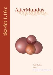
Tkz-Euclide and Tkz-Fct
In France, Alain Matthes is currently developing two packages that use
fairly intuitive syntax when drawing geometrical figures and plotting
functions. The manuals are written in French, but the examples are in
English.
The first package is called tkz-euclide. This is an exciting project that
entails numerous macros for creating geometrical figures.
The second package is called tkz-fct. This package of macros greatly
simplifies the plotting of functions.
David Arnold (CR) Using TIKZ November 20, 2010 24 / 24