MBA 604 Introduction Probaility and Statistics Lecture Notes

More documents

Recommendations

Info

$Inleiding tot LATEX$

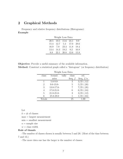
2 Graphical Methods Frequency and relative frequency distributions (Histograms): Example Weight Loss Data 20.5 19.5 15.6 24.1 9.9 15.4 12.7 5.4 17.0 28.6 16.9 7.8 23.3 11.8 18.4 13.4 14.3 19.2 9.2 16.8 8.8 22.1 20.8 12.6 15.9 Objective: Provide a useful summary of the available information. Method: Construct a statistical graph called a “histogram” (or frequency distribution) Weight Loss Data class bound- tally class rel. aries freq, f freq, f/n 1 5.0-9.0- 3 3/25 (.12) 2 9.0-13.0- 5 5/25 (.20) 3 13.0-17.0- 7 7/25 (.28) 4 17.0-21.0- 6 6/25 (.24) 5 21.0-25.0- 3 3/25 (.12) 6 25.0-29.0 1 1/25 (.04) Totals 25 1.00 Let k = # of classes max = largest measurement min = smallest measurement n =samplesize w =classwidth Rule of thumb: -The number of classes chosen is usually between 5 and 20. (Most of the time between 7 and 13.) -The more data one has the larger is the number of classes. 7
Formulas: Note: w = 28.6−5.4 6 w = 29−5 6 =4.0 (why?) k =1+3.3log10(n); w = =3.87. But we used max − min . k Graphs: Graph the frequency and relative frequency distributions. Exercise. Repeat the above example using 12 and 4 classes respectively. Comment on the usefulness of each including k =6. Steps in Constructing a Frequency Distribution (Histogram) 1. Determine the number of classes 2. Determine the class width 3. Locate class boundaries 4. Proceed as above Possible shapes of frequency distributions 1. Normal distribution (Bell shape) 2. Exponential 3. Uniform 4. Binomial, Poisson (discrete variables) Important -The normal distribution is the most popular, most useful, easiest to handle - It occurs naturally in practical applications - It lends itself easily to more in depth analysis Other Graphical Methods -Statistical Table: Comparing different populations - Bar Charts - Line Charts - Pie-Charts - Cheating with Charts 8
Page 1 and 2: MBA 604 Introduction Probaility and
Page 3 and 4: Contents 1 Data Analysis 5 1 Introd
Page 5 and 6: 10 Simple Linear Regression and Cor
Page 7: 7. How to interpret polls. How many
Page 11 and 12: If n is even, the median is the ave
Page 13 and 14: II. Measures of Variability Given:
Page 15 and 16: x x 2 90 8100 85 7225 65 4225 75 56
Page 17 and 18: (iii) Approximation: s range 4 (iv
Page 19 and 20: z = x − µ σ Example. A set of g
Page 21 and 22: (i) Complete all entries in the tab
Page 23 and 24: Chapter 2 Probability Contents. Sam
Page 25 and 26: nA = frequency of the event A nA n
Page 27 and 28: provided P (B) > 0. Similarly, P (B
Page 29 and 30: Thus only 32 percent of those perso
Page 31 and 32: (which is equal to Combinations For
Page 33 and 34: 2. Suppose that S = {1, 2, 3, 4, 5,
Page 35 and 36: (Hint: Start by defining the events
Page 37 and 38: The variable X transforms the probl
Page 39 and 40: 3 Discrete Distributions Binomial.
Page 41 and 42: of D elements of the first kind and
Page 43 and 44: One equation is redundant. Choose t
Page 45 and 46: 4. A random variable X has the foll
Page 47 and 48: 1. List the properties for a binomi
Page 49 and 50: Chapter 4 Continuous Distributions
Page 51 and 52: Z-score: OR (simply) Conversely, X
Page 53 and 54: Exercise. Specialize the above resu
Page 55 and 56: 3. Let Z be a standard normal distr
Page 57 and 58: Chapter 5 Sampling Distributions Co
Page 59 and 60:
σ ˆP = S.E.( ˆ pq P )= n (iii)
Page 61 and 62:
(ii) Find the probability that the
Page 63 and 64:
Single Quantitative Population: µ
Page 65 and 66:
where σ is estimated by s. Note: I
Page 67 and 68:
The width of the CI decreases. The
Page 69 and 70:
Please show all work. No credit for
Page 71 and 72:
Chapter 7 Large-Sample Tests of Hyp
Page 73 and 74:
Conclusion: At 100α% significance
Page 75 and 76:
1. Large sample (np ≥ 5,nq≥ 5)
Page 77 and 78:
Test: Sample 2: n2, x2, ˆp2 = x2 n
Page 79 and 80:
orders were recorded, with a sample
Page 81 and 82:
1. Sampled population is normal 2.
Page 83 and 84:
Sample data: Sample 1: n1, x1,s1 Sa
Page 85 and 86:
SUBC> alternative 1. Note: alternat
Page 87 and 88:
RR: Reject H0 if t>2.776 or t X 2
Page 89 and 90:
Q1: Do the data present sufficient
Page 91 and 92:
Training Group 1 2 3 4 65 75 59 94
Page 93 and 94:
GT: Grand Total. Computational Form
Page 95 and 96:
Treatments t1 t2 t3 Bi s1 17 34 23
Page 97 and 98:
Solution to (ii) Test. H0 : µ1 =
Page 99 and 100:
Chapter 10 Simple Linear Regression
Page 101 and 102:
3. The r.v. ɛ has a normal distrib
Page 103 and 104:
Optional material Ad Sales Calculat
Page 105 and 106:
Estimator mean: µ β1 ˆ = β1 Est
Page 107 and 108:
(ii) The population coefficient of
Page 109 and 110:
The regression equation is y=46.5 +
Page 111 and 112:
Source DF SS MS F P Regression 7626
Page 113 and 114:
4. The random components of any two
Page 115 and 116:
MINITAB. Use REGRESS command to reg
Page 117:
Q1. What is the prediction equation
show all

MBA 604 Introduction Probaility and Statistics Lecture Notes

You also want an ePaper? Increase the reach of your titles

Delete template?

Save as template?