Statistical Analysis of the CAPM I. Sharpe–Linter CAPM

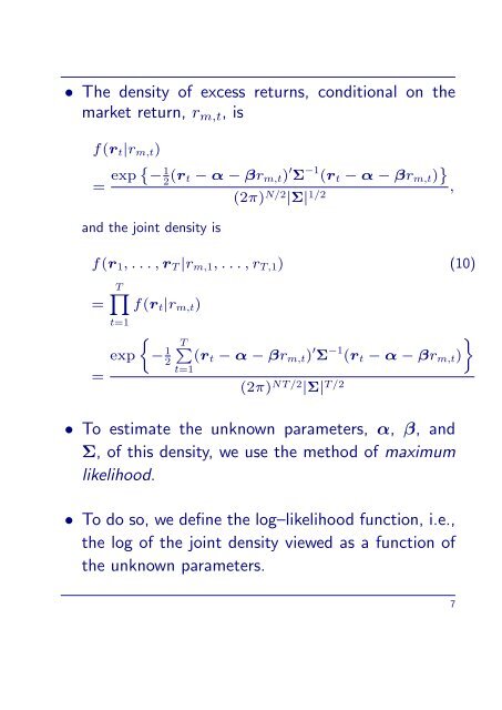
• The density of excess returns, conditional on the
market return, rm,t, is
f(rt|rm,t)
= exp { −1 2 (rt − α − βrm,t) ′ Σ −1 (rt − α − βrm,t) }
,
and the joint density is
(2π) N/2 |Σ| 1/2
f(r1, . . . , rT |rm,1, . . . , rT,1) (10)
=
=
T∏
t=1
exp
f(rt|rm,t)
{
− 1
2
T∑
(rt − α − βrm,t) ′ Σ −1 }
(rt − α − βrm,t)
t=1
(2π) NT/2 |Σ| T/2
• To estimate the unknown parameters, α, β, and
Σ, of this density, we use the method of maximum
likelihood.
• To do so, we define the log–likelihood function, i.e.,
the log of the joint density viewed as a function of
the unknown parameters.
7