Wavelet Galerkin Solutions of Ordinary Differential Equations
Wavelet Galerkin Solutions of Ordinary Differential Equations
Wavelet Galerkin Solutions of Ordinary Differential Equations

You also want an ePaper? Increase the reach of your titles
YUMPU automatically turns print PDFs into web optimized ePapers that Google loves.
Int. Journal <strong>of</strong> Math. Analysis, Vol. 5, 2011, no. 9, 407 - 424<br />
<strong>Wavelet</strong> <strong>Galerkin</strong> <strong>Solutions</strong> <strong>of</strong><br />
<strong>Ordinary</strong> <strong>Differential</strong> <strong>Equations</strong><br />
Vinod Mishra 1 and Sabina 2<br />
Sant Longowal Institute <strong>of</strong> Engineering and Technology<br />
Longowal 148 106 Punjab, India<br />
1 vinodmishra.2011@rediffmail.com, 2 sabinajindal8@gmail.com<br />
Abstract. Advantage <strong>of</strong> wavelet <strong>Galerkin</strong> method over finite difference or element<br />
method has led to tremendous applications in science and engineering. In recent<br />
years there has been increasing attempt to find solutions <strong>of</strong> differential equations<br />
using wavelet techniques. In this paper, we elaborate the wavelet techniques and<br />
apply <strong>Galerkin</strong> procedure to analyse one dimensional harmonic wave equation as a<br />
test problem using fictitious boundary approach; overcoming Dianfeng et al. (1996)<br />
reservation at higher resolution. This could have been possible only after evaluating<br />
connection coefficients at various scales.<br />
Keywords. <strong>Wavelet</strong> <strong>Galerkin</strong> Method; Condition Number; Connection Coefficients;<br />
Moments; Harmonic Wave Equation.<br />
1. Introduction<br />
<strong>Wavelet</strong> functions have generated significant interest from both theoretical and<br />
applied research over the last few years. The name wavelet comes from the<br />
requirement that they should integrate to zero, waving above and below x-axis. The<br />
concepts for understanding wavelets were provided recently by Meyer, Mallat,<br />
Daubechies, and many others. Since then, the number <strong>of</strong> applications where wavelets<br />
have been used has exploded.<br />
Many different types <strong>of</strong> wavelet functions have been presented over the past few<br />
years. In this paper, the Daubechies family <strong>of</strong> wavelets will be considered due to<br />
their useful properties.<br />
Since the contribution <strong>of</strong> orthogonal bases <strong>of</strong> compactly supported wavelet by<br />
Daubechies (1988) and multiresolution analysis based fast wavelet transform<br />
algorithm by Belkin (1991), wavelet based approximation <strong>of</strong> ordinary differential
408 V. Mishra and Sabina<br />
equations gained momentum in attractive way. <strong>Wavelet</strong>s have the capability <strong>of</strong><br />
representing the solutions at different levels <strong>of</strong> resolutions, which make them<br />
particularly useful for developing hierarchical solutions to engineering problems.<br />
Among the approximations, wavelet <strong>Galerkin</strong> technique is the most frequently used<br />
scheme these days. Daubechies wavelets as bases in a <strong>Galerkin</strong> method to solve<br />
differential equations require a computational domain <strong>of</strong> simple shape. This has<br />
become possible due to the remarkable work by Latto et al. [1], Xu et al. [4],<br />
Williams et al. [5 & 6] and Amartunga et al. [10]. Yet there is difficulty in dealing<br />
with boundary conditions. So far problems with periodic boundary conditions or<br />
periodic distribution have been dealt successfully. Fictitious boundary approach with<br />
Dirichlet boundaries has been applied by Dianfeng et al. [11] in analysing SH wave,<br />
but found difficulty near resonance response. In this paper, it is overcome by finding<br />
connection coefficients at different scales. Remind that Latto et al. [1] provides<br />
connection coefficients for j=0 and N=6 only. A detailed exposition <strong>of</strong> problem with<br />
distinct boundaries is also dealt by Jordi Besora [8].<br />
2<br />
<strong>Wavelet</strong> (x)<br />
: An oscillatory function ( x) L ( R)<br />
with zero mean is a wavelet if<br />
it has the desirable properties:<br />
1. Smoothness: (x)<br />
is n times differentiable and that their derivatives are<br />
continuous.<br />
2. Localization: (x)<br />
is well localized both in time and frequency domains, i.e.,<br />
(x)<br />
and its derivatives must decay very rapidly. For frequency localization ˆ<br />
( )<br />
must decay sufficiently fast as and that ˆ ( )<br />
becomes flat in the<br />
neighborhood <strong>of</strong> 0 . The flatness is associated with number <strong>of</strong> vanishing<br />
moments <strong>of</strong> (x)<br />
, i.e.<br />
<br />
x x dk<br />
<br />
k<br />
( ) =0 or equivalently ˆ<br />
( )<br />
0<br />
k<br />
k<br />
d<br />
for k 0,<br />
1,<br />
........., n<br />
d<br />
in the sense that larger the number <strong>of</strong> vanishing moments more is the flatness when<br />
is small.<br />
3. The admissibility condition<br />
<br />
<br />
<br />
ˆ<br />
( )<br />
<br />
suggests that<br />
2<br />
d<br />
<br />
2<br />
ˆ( )<br />
decays at least as<br />
1<br />
or<br />
1<br />
x for 0 .<br />
Daubechies <strong>Wavelet</strong>. Daubechies wavelets are compactly supported functions. This<br />
means that they have non zero values within a finite interval and have a zero value
<strong>Wavelet</strong> <strong>Galerkin</strong> solutions 409<br />
everywhere else. That’s why it is useful for representing the solution <strong>of</strong> differential<br />
equation. In 1988, Ingrid Daubechies defined scaling function as<br />
( x)<br />
N 1<br />
<br />
k0<br />
a (<br />
2x<br />
k),<br />
k<br />
where N denotes the genus <strong>of</strong> the Daubechies wavelet. The functions generated<br />
with these coefficients will have supp [ 0,<br />
N 1]<br />
and ( N / 2 1)<br />
vanishing wavelet<br />
moments.<br />
Sometimes the scaling functions are defined as<br />
N 1<br />
( x)<br />
2<br />
c ( 2x<br />
k),<br />
<br />
<br />
<br />
k0<br />
k<br />
where ak 2ck<br />
, with the property that N 1<br />
c k 2 .<br />
k0<br />
We have computed the Daubechies coefficients for N=4, 6, 8, 10, 12 in the Table<br />
given below:<br />
k<br />
N=4<br />
Table 1.1: Daubechies <strong>Wavelet</strong> Filter Coefficients c k<br />
N=6<br />
N=8<br />
N=10<br />
N=12<br />
N=14<br />
0 0.4830 0.3327 0.2304 0.1601 0.1115 0.0779<br />
N=16<br />
0.0544<br />
1 0.8365 0.8069 0.7148 0.6038 0.4946 0.3965 0.3129<br />
2 0.2241 0.4599 0.6309 0.7243 0.7511 0.7291 0.6756<br />
3 -0.1294 -0.1350 -0.0280 0.1384 0.3153 0.4698 0.5854<br />
4 -0.0854 -0.1870 -0.2423 -0.2263 -0.1439 -0.0158<br />
5 0.0352 0.0308 -0.0322 -0.1298 -0.2240 -0.2840<br />
6 0.0329 0.0776 0.0975 0.0713 0.0005<br />
7 -0.0106 -0.0062 0.0275 0.0806 0.1287<br />
8 -0.0126 -0.0316 -0.0380 -0.0174<br />
9 0.0033 0.0006 -0.0166 -0.0441<br />
10 0.0048 0.0126 0.0140<br />
11 -0.0011 0.0004 0.0087<br />
12 -0.0018 -0.0049<br />
13 0.0004 -0.0004<br />
14 0.0007<br />
15 -0.0001<br />
The associated wavelet function is given by
410 V. Mishra and Sabina<br />
1<br />
k<br />
( x)<br />
( 1)<br />
a1k<br />
( 2x<br />
k)<br />
.<br />
<br />
k 2<br />
N<br />
2. <strong>Wavelet</strong> <strong>Galerkin</strong> Technique<br />
<strong>Galerkin</strong> Method. It was Russian engineer V.I. <strong>Galerkin</strong> who proposed a projection<br />
method based on weak form. In it a set <strong>of</strong> test functions are selected such that<br />
residual <strong>of</strong> differential equation becomes orthogonal to test functions [8].<br />
Consider one-dimensional differential equation [12, pp. 451-479]<br />
Lu ( x)<br />
f ( x),<br />
0 x 1<br />
(2.1)<br />
with Dirichlet boundary conditions<br />
u( 0)<br />
a,<br />
u(<br />
1)<br />
b.<br />
f is real valued and continuous functions <strong>of</strong> x on [0,1]. L is a uniformly elliptic<br />
differential operator.<br />
L 2 ([0, 1]) is a Hilbert space with inner product<br />
<br />
Suppose that j <br />
is<br />
1<br />
f , g<br />
f ( x)<br />
g(<br />
x)<br />
dt.<br />
2<br />
C on [0, 1] such that<br />
v j 0)<br />
a,<br />
v j ( 1)<br />
<br />
0<br />
v is a complete orthonormal system for L 2 ([0, 1]) and that every j v<br />
( b.<br />
Select a finite set <strong>of</strong> indices j and consider the subspace<br />
S span v j : j <br />
<br />
Let the approximate solution u s <strong>of</strong> the given equation be<br />
us xk<br />
vk<br />
S.<br />
<br />
k<br />
(2.2)<br />
We would like to determine xk in a way that us behaves as if is a true solution on S,<br />
i.e.<br />
u , v f , v j <br />
(2.3)<br />
L s j<br />
j<br />
such that the boundary conditions u s ( 0)<br />
u s ( 1)<br />
0 are satisfied. Substituting u s in<br />
(2.3),<br />
v , v x<br />
f , v j .<br />
(2.4)<br />
<br />
k<br />
L k j k<br />
j<br />
Let X and Y denote the vectors x k and , ,<br />
k<br />
k f v<br />
k<br />
k<br />
A <br />
a j k j , k<br />
, , where a j,<br />
k Lv<br />
k , v j .<br />
(2.4) reduces to the system <strong>of</strong> linear equations<br />
y and A the matrix
<strong>Wavelet</strong> <strong>Galerkin</strong> solutions 411<br />
<br />
k<br />
a x y<br />
j,<br />
k k j or equivalently AX = Y . (2.5)<br />
Thus in <strong>Galerkin</strong> method, for each subset , we find an approximation u s in S to u<br />
by solving (2.5) for X and then substituting its components in (2.2). It is expected<br />
that as we increase in some systematic way, us converges to u, the actual solution.<br />
Condition Number <strong>of</strong> a Matrix. We know that a linear system AX Y has a<br />
unique solution X for every Y if a square matrix A is invertible. It is <strong>of</strong>ten observed<br />
that for two close values <strong>of</strong> Y andY ',<br />
X and X ' are far apart. Such a linear system<br />
is called badly conditioned. Thus data Y is expected to be fairly accurate. Condition<br />
number <strong>of</strong> A is given by<br />
1<br />
( A)<br />
A A , C ( A)<br />
1 .<br />
C <br />
#<br />
#<br />
Thus # ( ), A C is the measure <strong>of</strong> stability <strong>of</strong> the linear system under perturbation <strong>of</strong> the<br />
data Y . Small condition number near 1 is desirable. In case it is high, replace the<br />
system by equivalent system BAX BY , B is a preconditioning matrix such that<br />
C# ( BA)<br />
C#<br />
( A)<br />
.<br />
To facilitate easy calculation, A is considered to be sparse, i.e., A should have high<br />
proportion <strong>of</strong> entries 0. The best one is when A is in diagonal form.<br />
<strong>Wavelet</strong> <strong>Galerkin</strong> method<br />
j / 2 j<br />
Let j,<br />
k ( x)<br />
2 ( 2 x k)<br />
be a wavelet basis for<br />
conditions<br />
2<br />
L ([ 0,<br />
1])<br />
with boundary<br />
0)<br />
( 1)<br />
0.<br />
j,<br />
k ( j,<br />
k<br />
For each ( j , k)<br />
,<br />
j,<br />
k is<br />
The scale <strong>of</strong> approximates<br />
2<br />
C .<br />
j<br />
2 and is centralized near point k<br />
j <br />
2 and equates<br />
to zero outside the interval centred at k<br />
j <br />
2 <strong>of</strong> length proportional to 2 .<br />
j <br />
In <strong>Wavelet</strong> <strong>Galerkin</strong> method equations (2.2) and (2.3) may thus be replaced by<br />
x<br />
and<br />
u s<br />
j,<br />
k j,<br />
k<br />
j,<br />
k<br />
<br />
<br />
<br />
j,<br />
k<br />
L<br />
j,<br />
k , l,<br />
m x<br />
j,<br />
k f , l,<br />
m <br />
( l,<br />
m)<br />
.<br />
So that AX Y.<br />
(2.6)<br />
Where A= a , X ( x j,<br />
k ) ( j,<br />
k ) <br />
, Y ( yl<br />
, m ) ( l,<br />
m)<br />
<br />
.<br />
l,<br />
m;<br />
j,<br />
k ( l,<br />
m),<br />
( j,<br />
k ) <br />
In it a l,<br />
m;<br />
j,<br />
k L<br />
j,<br />
k , l,<br />
m , yl , m f , l,<br />
m .<br />
The pairs (l,m) and (j,k) represent respectively row and column <strong>of</strong> A.<br />
Consider A to be sparse. Represent AX Y by equivalent
412 V. Mishra and Sabina<br />
MZ V<br />
(2.7)<br />
in which case M has relatively low condition number, if A has not. This system is<br />
now well conditioned. Again M to be sparse is desirable.<br />
The matrix M in the preconditioned system (4.6) has condition number bounded<br />
independently <strong>of</strong> . So as we increase to approximate solution with more<br />
accuracy, the condition number maintains it boundedness, which is much better than<br />
2<br />
the finite difference method in which case condition number grows as N . Thus the<br />
data errors, may be due to rounding <strong>of</strong>f, has no effect in wavelet <strong>Galerkin</strong> solution<br />
over [0, 1] as we approach for better and better accuracy.<br />
3. Connection Coefficients<br />
In order to find the solution <strong>of</strong> differential equation by using wavelet <strong>Galerkin</strong><br />
method there is need to find the connection coefficients as explored in Latto et al. [1]<br />
as<br />
<br />
l1l2<br />
<br />
<br />
d1d2<br />
d1<br />
d 2<br />
( x)<br />
( x)<br />
dx.<br />
(3.1)<br />
l1<br />
l2<br />
Taking derivatives <strong>of</strong> the scaling function d times. we get<br />
1<br />
<br />
0<br />
N<br />
k<br />
d<br />
d<br />
d<br />
( x) 2 a ( 2x<br />
k)<br />
.<br />
(3.2)<br />
k<br />
k<br />
d1d2<br />
After simplification and considering it for all , gives a system <strong>of</strong> linear<br />
equations with<br />
d1d<br />
2 as unknown vector:<br />
1 2<br />
d1d2<br />
T d1d<br />
,<br />
d 1<br />
2<br />
1 d d d and a ia q<br />
l<br />
where 2<br />
T 2 i .<br />
i<br />
k<br />
The moments M i <strong>of</strong> i are defined as<br />
<br />
k k<br />
M i x i<br />
<br />
0<br />
0 <br />
( x)<br />
dx<br />
with M 1.<br />
Latto et al. [1] derives a formula to compute the moments by induction on k.<br />
j<br />
t1<br />
N 1<br />
j 1 j jt<br />
t<br />
<br />
tl<br />
<br />
M<br />
i <br />
,<br />
2(<br />
2 1)<br />
i <br />
a<br />
ii<br />
j<br />
t0<br />
t<br />
l0<br />
l<br />
<br />
i0<br />
<br />
where the ai s are the Daubechies wavelet coefficients.<br />
Finally the system will be<br />
l1l2
<strong>Wavelet</strong> <strong>Galerkin</strong> solutions 413<br />
1<br />
d<br />
<br />
2<br />
d<br />
M<br />
<br />
<br />
<br />
<br />
T I 1 d1d<br />
2<br />
0<br />
<br />
.<br />
!<br />
<br />
d <br />
Matlab s<strong>of</strong>tware is used to compute the connection coefficients and moments at<br />
different scales. We have computed the connection coefficients by substituting the<br />
values <strong>of</strong> Daubechies coefficients in the matrix T and by evaluating moments by<br />
using the programme that is given in [8].<br />
Latto et al. [1] computed the connection coefficients at j=0 and N=6 only. We have<br />
computed the connection coefficients at all values <strong>of</strong> j and N. The values <strong>of</strong><br />
connection coefficients, for example, at j=0, 4, 7 and N=6 and at j=5 and N=12 are<br />
shown in Table 3.1.<br />
Table 3.1: 2- term connection coefficients<br />
Connection Coefficients at N=6, j=0, d1=2, d2=0<br />
[ 4]<br />
5.357142857144194e-003<br />
[ 3]<br />
1.142857142857108e-001<br />
[ 2]<br />
-8.761904761904359e-001<br />
[ 1]<br />
3.390476190476079e+000<br />
[ 0]<br />
-5.267857142857051e+000<br />
[ 1]<br />
3.390476190476190e+000<br />
[ 2]<br />
-8.761904761904867e-001<br />
[ 3]<br />
1.142857142857139e-001<br />
[ 4]<br />
5.357142857141956e-003<br />
Connection Coefficients at N=6, j=7, d1=2, d2=0<br />
[ 4]<br />
8.777142857143141e+001<br />
[ 3]<br />
1.872457142857136e+003<br />
[ 2]<br />
-1.435550476190484e+004<br />
[ 1]<br />
5.554956190476204e+004<br />
[ 0]<br />
-8.630857142857112e+004<br />
[ 1]<br />
5.554956190476144e+004<br />
[ 2]<br />
-1.435550476190458e+004<br />
[ 3]<br />
1.872457142857130e+003<br />
[ 4]<br />
8.777142857143379e+001
414 V. Mishra and Sabina<br />
Connection Coefficients at N=12, j=5, d=2<br />
[ 10]<br />
-1.294452960894988e-008<br />
[ 9]<br />
<br />
2.693100643685327e-005<br />
[ 8]<br />
-3.549272110888916e-003<br />
[ 7]<br />
-5.566810017417083e-002<br />
[ 6]<br />
-6.727300176318085e-002<br />
[ 5]<br />
6.633534506945016e+000<br />
[ 4]<br />
-5.054628929484702e+001<br />
[ 3]<br />
2.098232006991124e+002<br />
[ 2]<br />
-6.458708407940719e+002<br />
[ 1]<br />
2.367351361198240e+003<br />
[ 0]<br />
-3.774529005718791e+003<br />
[ 1]<br />
2.367351361198260e+003<br />
[ 2]<br />
-6.458708407940832e+002<br />
[ 3]<br />
2.098232006991146e+002<br />
[ 4]<br />
-5.054628929484773e+001<br />
[ 5]<br />
<br />
6.633534506945424e+000<br />
[ 6]<br />
-6.727300176361031e-002<br />
[ 7]<br />
-5.566810017416311e-002<br />
[ 8]<br />
-3.549272110869743e-003<br />
[ 9]<br />
2.693100643242748e-005<br />
[ 10]<br />
-1.294445771987477e-008<br />
4. <strong>Wavelet</strong> Methods for ODE<br />
Consider the equation [Amaratunga et al.]<br />
2<br />
u<br />
u f ,<br />
(4.1)<br />
2<br />
x<br />
where u , f are periodic in x <strong>of</strong> period d Z .<br />
The <strong>Wavelet</strong> Galerikin solution <strong>of</strong> periodic problem is slightly more complicated<br />
than the finite difference approach as the former involves solving a set <strong>of</strong>
<strong>Wavelet</strong> <strong>Galerkin</strong> solutions 415<br />
simultaneous equations in wavelet space and not in physical space. The solution in<br />
wavelet space is then transformed back to physical space by FTT.<br />
Let the wavelet expansion u(x) at scale j be<br />
j / 2 j<br />
u(<br />
x)<br />
c 2 ( 2 x k)<br />
, k Z,<br />
(4.2)<br />
k<br />
k<br />
where ck s are periodic wavelet coefficients <strong>of</strong> u, periodic in x.<br />
j<br />
Put y 2 x so that<br />
U ( y)<br />
u(<br />
x)<br />
C ( y k),<br />
C 2<br />
k<br />
k<br />
k<br />
If d is the period <strong>of</strong> u, then U (y)<br />
and so also Ck is periodic in y with period 2 d.<br />
j<br />
j / 2<br />
j<br />
Let us discretize U(y ) at all dyadic points x y y Z<br />
<br />
2 ,<br />
U i C k<br />
ik<br />
C<br />
ik<br />
k , i 0,<br />
1,<br />
2,....,<br />
n 1.<br />
k<br />
k<br />
The matrix representation is U k<br />
* C , where k is the convolution kernal, i.e. the<br />
first column <strong>of</strong> the scaling function matrix.<br />
Similarly the wavelet expansion for f (x),<br />
j / 2 j<br />
f ( x)<br />
d 2 ( 2 x k)<br />
, k Z.<br />
(4.3)<br />
k<br />
k<br />
j / 2<br />
f ( x)<br />
Dk<br />
( y k),<br />
Dk<br />
2 dk<br />
.<br />
k<br />
F(<br />
y)<br />
<br />
And the matrix representation is<br />
F k<br />
* D.<br />
Substitute the expansions <strong>of</strong> u(x) and f (x)<br />
in (4.1) and then take inner product on<br />
both sides with ( y j),<br />
j Z .<br />
( n)<br />
Use j k<br />
<br />
( y k)<br />
(<br />
y j)<br />
dy and jk (<br />
y k)<br />
(<br />
y j)<br />
dx , we obtain<br />
k . C g.<br />
Now take Fourier Transforms<br />
Uˆ kˆ<br />
. Cˆ<br />
.<br />
Fˆ kˆ<br />
. Dˆ<br />
.<br />
kˆ . Cˆ<br />
gˆ<br />
.<br />
Subsequently, Uˆ<br />
Fˆ<br />
/ kˆ<br />
. Inverse FT will give U.<br />
Wherein . and / denote component by component multiplication and division<br />
respectively.<br />
c<br />
k<br />
.
416 V. Mishra and Sabina<br />
Fictitious Boundary Approach [Dianfeng et al.]<br />
Consider the equation<br />
2<br />
u<br />
<br />
u 0,<br />
x [<br />
0,<br />
1]<br />
(4.4)<br />
2<br />
x<br />
with Dirichlet’s boundaries u ( 0),<br />
u(<br />
1).<br />
j<br />
u in (4.2) is periodic in x <strong>of</strong> period d Z (k varies from –N+1 to 2 ).<br />
The boundaries <strong>of</strong> the support <strong>of</strong> (4.2) are N 1<br />
j and<br />
j<br />
N 2<br />
. Subsequently, the<br />
original boundaries 0 and 1 now changes to the Fictitious Boundaries, i.e. boundary<br />
N 1<br />
on both sides <strong>of</strong> 0 and 1 are extended by an amount ,<br />
( 0)<br />
<br />
( N 1)<br />
N<br />
1<br />
j <br />
j<br />
N 1<br />
2 u<br />
j <br />
u 2<br />
2<br />
N 1<br />
without affecting the solution within [0,1], the affected solution is within , 0]<br />
j<br />
N 2<br />
and [ 1,<br />
] . The equation (4.4) now reduces to<br />
2<br />
1<br />
j<br />
2<br />
2 j<br />
j<br />
2<br />
<br />
k<br />
N<br />
1<br />
j<br />
2<br />
2<br />
j<br />
2<br />
1<br />
j<br />
2<br />
[ j<br />
2<br />
Ck<br />
''(<br />
y k)<br />
C<br />
k(<br />
y k)<br />
0.<br />
(4.5)<br />
k<br />
N 1<br />
Inner product is taken on both sides <strong>of</strong> (4.5) with ( y n)<br />
taking the integration<br />
j<br />
N 1<br />
N 12<br />
limits to , . We obtain<br />
j<br />
2<br />
j<br />
2<br />
2 2 j<br />
<br />
k<br />
k<br />
jk<br />
C j<br />
C 0.<br />
(4.6)<br />
The Dirichlet boundary conditions give equations<br />
i<br />
2<br />
k<br />
k<br />
N 1<br />
i<br />
2<br />
k<br />
k<br />
N 1<br />
C ( k)<br />
u(<br />
0).<br />
(4.7a)<br />
C ( 1<br />
k)<br />
u(<br />
1).<br />
(4.7b)<br />
Take inner product with ( l)<br />
and (<br />
1 l)<br />
i<br />
2<br />
k<br />
k<br />
N<br />
1<br />
respectively reducing the left boundary<br />
condition to C ( 0)<br />
u(<br />
0)<br />
and C ( 1)<br />
u(<br />
1).<br />
First and last equations<br />
lk<br />
i<br />
2<br />
k<br />
k<br />
N<br />
1<br />
are replaced by the following equations. The place <strong>of</strong> corresponding connection<br />
coefficients in first row and last row are determined by the delta function.<br />
Appropriate connection coefficients are used to solve the ill-conditioned system for<br />
C .<br />
k<br />
Capacitance Matrix and the Boundary Conditions [Amaratunga et al.]<br />
Consider the equation (4.1) defined over [a,b] with Dirichlet boundary conditions<br />
lk
<strong>Wavelet</strong> <strong>Galerkin</strong> solutions 417<br />
u( a)<br />
u a &u(<br />
b)<br />
ub.<br />
Let u and f are periodic with period d , 0 a b d .<br />
If f is not periodic, it can be make periodic making it zero or extending smoothly<br />
outside [ a , b].<br />
Let v(x) be the solution in [ a, b]<br />
with periodic boundary conditions.<br />
The solution u (x)<br />
with Dirichlet boundary conditions is by adding another functions<br />
w (x)<br />
such that<br />
u v w.<br />
(4.8)<br />
2 2<br />
v w<br />
From (18) <br />
v w f , i.e.<br />
2 2<br />
x<br />
x<br />
2<br />
w<br />
w<br />
0 in a ,b.<br />
2<br />
x<br />
However on or outside [ a , b],<br />
wxx<br />
may take such values as to make u satisfy the<br />
given boundary conditions. The desired effect may be achieved by placing sources<br />
(or delta functions) along the boundary [ 0,<br />
d ] which encompasses [ a , b]<br />
. In other<br />
words, we need the solution w to<br />
2<br />
w<br />
<br />
w X in [ 0,<br />
d ],<br />
2<br />
x<br />
where X ( x)<br />
X ( x a)<br />
X ( x b).<br />
X a<br />
b<br />
a X b<br />
X , are constants, and stands for delta function.<br />
Now Green’s function G (x)<br />
(or impulse response) <strong>of</strong> the differential equation is<br />
given by<br />
2<br />
G<br />
G ( x).<br />
2<br />
x<br />
So the solution w G(<br />
x)<br />
* X ( x)<br />
X aG(<br />
x a)<br />
X bG(<br />
x b).<br />
(4.9)<br />
From (4.8) and (4.9)<br />
( a)<br />
X G(<br />
o)<br />
X G(<br />
a b)<br />
u v(<br />
a).<br />
w a<br />
b<br />
a<br />
w b)<br />
X aG(<br />
b a)<br />
X bG(<br />
o)<br />
ub<br />
(<br />
Equivalently,<br />
v(<br />
b).<br />
G(<br />
o)<br />
<br />
G(<br />
b a)<br />
G(<br />
a b)<br />
<br />
X a ua<br />
v(<br />
a)<br />
<br />
.<br />
G(<br />
o)<br />
<br />
<br />
( )<br />
<br />
<br />
X b ub<br />
v b <br />
Solving for X a , X b , the solution w is obtained.
418 V. Mishra and Sabina<br />
Offsetting the boundary sources. Placing the sources at the boundary in the wavelet<br />
method amounts to large error due to finite support <strong>of</strong> ; i.e, number <strong>of</strong> non zero<br />
wavelet coefficients. Actually, support <strong>of</strong> in wavelet space is equal to support <strong>of</strong><br />
that is used to define it.<br />
( x ) g k(<br />
y k),<br />
k<br />
where wavelet coefficients<br />
m<br />
g 2 ( k)<br />
.<br />
k<br />
m<br />
Number <strong>of</strong> wavelet coefficients 2 d.<br />
The magnitude s <strong>of</strong> the <strong>of</strong>fset is so chosen that number <strong>of</strong> discritization point<br />
involved is at least equal to the support <strong>of</strong> scaling function<br />
Suppose<br />
a1 a s,<br />
b1<br />
b s .<br />
Then X X a<br />
( x a1)<br />
X b<br />
( x b1<br />
) so that X a , X b are solutions <strong>of</strong><br />
G(<br />
a a1)<br />
G(<br />
a b1<br />
) X<br />
a ua<br />
v(<br />
a)<br />
<br />
<br />
.<br />
( 1)<br />
( 1)<br />
<br />
<br />
( )<br />
<br />
G<br />
b a G b b <br />
X b ub<br />
v b <br />
5. Test Problem<br />
We apply fictitious boundary approach to analyse harmonic wave (differential)<br />
equation:<br />
2<br />
u<br />
<br />
u 0,<br />
x [<br />
0,<br />
1]<br />
(5.1)<br />
2<br />
x<br />
with Dirichlet boundary conditions u( 0)<br />
1<br />
and u ( 1)<br />
0 . 훼 = (9.5휋) = 891.<br />
In [8], this problem has been treated with boundary u( 0)<br />
1<br />
& u ( 1)<br />
0 .<br />
Exact solution is: 푢 = 푐표푠√훼 푥 − 푐표푡√훼 푠푖푛√훼 푥.<br />
j<br />
2<br />
j / 2 j<br />
Let the solution be u(<br />
x)<br />
c k 2 ( 2 x k)<br />
.<br />
k <br />
N 1<br />
Fictitious boundary approach is applied in which original boundary [0,1] is extended<br />
N 1<br />
on both ends by margin j . Proceeding as in Latto et al. [1], (5.1) reduces to<br />
2<br />
C<br />
k n, k C<br />
k<br />
n,<br />
k 0<br />
(5.2)<br />
where<br />
and<br />
k<br />
j<br />
( 2 x n)<br />
(<br />
2<br />
n , k<br />
k<br />
j<br />
x k)<br />
dx
0<br />
<br />
<br />
<br />
:<br />
. <br />
<br />
:<br />
<br />
<br />
0<br />
<strong>Wavelet</strong> <strong>Galerkin</strong> solutions 419<br />
j<br />
j<br />
n , k <br />
( 2 x n)<br />
(<br />
2 x k)<br />
dx .<br />
We compute the solution <strong>of</strong> equation (5.2) by replacing the first and last equations<br />
by the equations obtained by using the right and left boundaries which also represent<br />
the relations <strong>of</strong> the coefficients ck as explained in Section 4. After replacing the rows,<br />
we get the following matrix form with N=6:<br />
1<br />
4<br />
0<br />
<br />
:<br />
:<br />
0<br />
<br />
0<br />
<br />
3<br />
where C =<br />
0<br />
<br />
1<br />
:<br />
. ..<br />
:<br />
...<br />
C5<br />
<br />
<br />
<br />
C<br />
4 <br />
C<br />
3<br />
<br />
C<br />
2 <br />
C<br />
<br />
1<br />
<br />
:<br />
<br />
:<br />
<br />
<br />
j C<br />
2 <br />
...<br />
...<br />
:<br />
...<br />
:<br />
0<br />
j<br />
1*(<br />
2 6)<br />
0<br />
0<br />
:<br />
...<br />
:<br />
0<br />
TC 0<br />
0<br />
<br />
:<br />
<br />
:<br />
4<br />
0<br />
0<br />
<br />
0 ... 0 0<br />
0 ... 0 0<br />
<br />
<br />
: : : : <br />
<br />
0 ... ... 0<br />
: : : : <br />
<br />
0 .. . 0 0<br />
Now by applying Gauss elimination method and using the programming <strong>of</strong> Matlab<br />
this matrix can be easily solved. Thus solution is obtained directly by substituting the<br />
values <strong>of</strong> 푐 .<br />
1<br />
0<br />
:<br />
...<br />
:<br />
...<br />
...<br />
...<br />
:<br />
...<br />
:<br />
...<br />
0<br />
0<br />
:<br />
...<br />
:<br />
1<br />
0<br />
0<br />
:<br />
0<br />
:<br />
0<br />
j j<br />
( 2 4)*(<br />
2 6)
420 V. Mishra and Sabina<br />
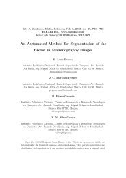
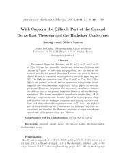
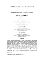
For N=8, j=8, the graph <strong>of</strong> solution <strong>of</strong> exact solution and wavelet solution<br />
2<br />
1<br />
0<br />
-1<br />
D8, 256 points.<br />
Exact solution<br />
WG Solution<br />
-2<br />
0<br />
0.015<br />
0.1 0.2 0.3 0.4 0.5<br />
x<br />
Error.<br />
0.6 0.7 0.8 0.9 1<br />
0.01<br />
0.005<br />
0<br />
0 0.1 0.2 0.3 0.4 0.5<br />
x<br />
0.6 0.7 0.8 0.9 1
<strong>Wavelet</strong> <strong>Galerkin</strong> solutions 421<br />
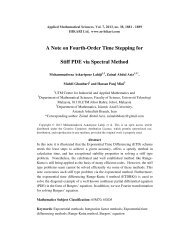
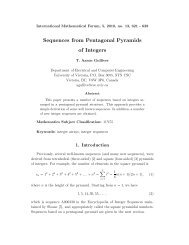
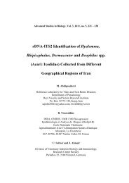
For N=6, j=8, the graph <strong>of</strong> solution <strong>of</strong> exact solution and wavelet solution<br />
2<br />
1<br />
0<br />
-1<br />
D6, 256 points.<br />
-2<br />
0<br />
0.015<br />
0.1 0.2 0.3 0.4 0.5<br />
x<br />
Error.<br />
0.6 0.7 0.8 0.9 1<br />
0.01<br />
0.005<br />
Exact solution<br />
WG solution<br />
0<br />
0 0.1 0.2 0.3 0.4 0.5<br />
x<br />
0.6 0.7 0.8 0.9 1
422 V. Mishra and Sabina<br />
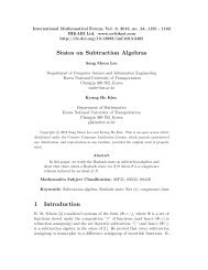
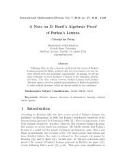
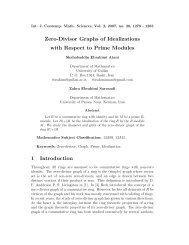
For N=6, j=9, graph shows that error decreases between exact and wavelet solution.<br />
2<br />
1<br />
0<br />
-1<br />
D6, 512 points.<br />
-2<br />
0 0.1 0.2 0.3 0.4 0.5<br />
x<br />
0.6 0.7 0.8 0.9 1<br />
x 10-3<br />
Error.<br />
4<br />
3<br />
2<br />
1<br />
Exact solution<br />
WG solution<br />
0<br />
0 0.1 0.2 0.3 0.4 0.5<br />
x<br />
0.6 0.7 0.8 0.9 1
<strong>Wavelet</strong> <strong>Galerkin</strong> solutions 423<br />
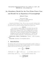
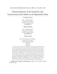
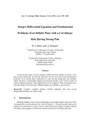
For N=12, j=10, graph shows that error decreases between exact and wavelet<br />
solution.<br />
2<br />
1<br />
0<br />
-1<br />
-2<br />
0 0.1 0.2 0.3 0.4 0.5<br />
x<br />
0.6 0.7 0.8 0.9 1<br />
x 10-4<br />
Error.<br />
8<br />
6<br />
4<br />
2<br />
6. Conclusion<br />
D12, 1024 points.<br />
Exact solution<br />
WG Solution<br />
0<br />
0 0.1 0.2 0.3 0.4 0.5<br />
x<br />
0.6 0.7 0.8 0.9 1<br />
The wavelet method has been shown to be a powerful numerical tool for the fast and<br />
accurate solution <strong>of</strong> differential equations. <strong>Solutions</strong> obtained using the Daubechies<br />
6, 8 and 12 coefficients wavelets have been compared with the exact solutions. In<br />
solving harmonic equation 훼 is chosen to be 891. Matching solutions are obtained<br />
for N=6, j=9 and N=12, j=10. Condition numbers for D12 are constantly lower than<br />
for D6, less errors are shown for former. Dianfeng et al. [11] is silent for higher<br />
values <strong>of</strong> resolution near resonance point but here good solution is shown to exist for<br />
D12.<br />
(<br />
t)<br />
N 1<br />
<br />
n0<br />
h(<br />
n)<br />
2<br />
1/<br />
2<br />
(<br />
2t<br />
n)
424 V. Mishra and Sabina<br />
References<br />
[1] A. Latto, H.L. Resnik<strong>of</strong>f and E. Tenenbaum, The Evaluation <strong>of</strong> Connection<br />
Coefficients <strong>of</strong> Compactly Supported <strong>Wavelet</strong>s, in: Proceedings <strong>of</strong> the French-USA<br />
Workshop on <strong>Wavelet</strong>s and Turbulence, Princeton, New York, 1991, Springer-<br />
Verlag, 1992.<br />
[2] Bjorn Jawerth and Wim Sweldens, <strong>Wavelet</strong>s Multiresolution Analysis Adapted<br />
for Fast Solution <strong>of</strong> Boundary Value <strong>Ordinary</strong> <strong>Differential</strong> <strong>Equations</strong>, Proc. 6 th Cop.<br />
Mount Multi. Conf., April 1993, NASA Conference Pub., 259--273.<br />
[3] G. Belkin, R. Coifman and V. Rokhlin, Fast <strong>Wavelet</strong> Transforms and Numerical<br />
Algorithms, Comm. Pure Appl. Math. 44 (1997), 141-183.<br />
[4] J.-C. Xu and W.-C. Shann, <strong>Wavelet</strong>-<strong>Galerkin</strong> Methods for Two-point Boundary<br />
Value Problems, Num. Math. Eng. 37(1994), 2703-2716.<br />
[5] J. R. Williams and K. Amaratunga, <strong>Wavelet</strong> Based Green’s Function Approach<br />
to 2D PDEs, Engg. Comput.10 (1993), 349-367.<br />
[6] J. R. Williams and K. Amaratunga, High Order wavelet Extrapolation Schemes<br />
for Initial Problems and Boundary Value Problems, July 1994, IESL Tech. Rep., No.<br />
94-07, Intelligent Engineering Systems Laboratory, MIT.<br />
[7] J.R. Williams and Kelvin Amaratunga, Simulation Based Design using <strong>Wavelet</strong>s,<br />
Intelligent Engineering Systems Laboratory, MIT (USA).<br />
[8] Jordi Besora, <strong>Galerkin</strong> <strong>Wavelet</strong> Method for Global Waves in 1D, Master Thesis,<br />
Royal Inst. <strong>of</strong> Tech. Sweden, 2004.<br />
[9] K. Amaratunga, J.R. Williams, S. Qian and J. Weiss, <strong>Wavelet</strong>-<strong>Galerkin</strong> solutions<br />
for one Dimensional Partial <strong>Differential</strong> <strong>Equations</strong>, IESL Technical Report No. 92-<br />
05, Intelligent Engineering Systems Laboratory, M. I. T ., 1992.<br />
[10] K. Amaratunga and J.R. William, <strong>Wavelet</strong>-<strong>Galerkin</strong> <strong>Solutions</strong> for Onedimensional<br />
Partial <strong>Differential</strong> <strong>Equations</strong>, Inter. J. Num. Meth. Eng. 37(1994),<br />
2703-2716.<br />
[11] L.U. Dianfeng, Tadashi Ohyoshi and Lin ZHU, Treatment <strong>of</strong> Boundary<br />
Condition in the Application <strong>of</strong> <strong>Wavelet</strong>–<strong>Galerkin</strong> Method to a SH Wave Problem,<br />
1996, Akita Univ. (Japan).<br />
[12] M.W. Frazier, An Introduction to <strong>Wavelet</strong>s through Linear Algebra, Springer,<br />
New York, 1999.<br />
[13] Stephan Dhalke and Ilona Weinreich, <strong>Wavelet</strong>-<strong>Galerkin</strong> Methods: An Adapted<br />
Biorthogonal <strong>Wavelet</strong> Basis, Constructive Approximation 9 (1993), 237-262.<br />
[14] Ole Christensen, Frames, Riesz Basdes, and Discrete Gabor/<strong>Wavelet</strong><br />
Expansions, Bulletin (New Series) <strong>of</strong> the American Mathematical Society 38 (2001),<br />
273-291.<br />
Received: September, 2010