Simply Sequentially Additive Labeling of Some Special Trees
Simply Sequentially Additive Labeling of Some Special Trees
Simply Sequentially Additive Labeling of Some Special Trees

You also want an ePaper? Increase the reach of your titles
YUMPU automatically turns print PDFs into web optimized ePapers that Google loves.
Applied Mathematical Sciences, Vol. 6, 2012, no. 131, 6501 - 6514<br />
<strong>Simply</strong> <strong>Sequentially</strong> <strong>Additive</strong> <strong>Labeling</strong><br />
<strong>of</strong> <strong>Some</strong> <strong>Special</strong> <strong>Trees</strong><br />
K. Manimekalai<br />
Department <strong>of</strong> Mathematics<br />
Bharathi Women’s College (Autonomous)<br />
Chennai − 600 108, India<br />
manimekalai2010@yahoo.com<br />
J. Baskar Babujee<br />
Department <strong>of</strong> Mathematics<br />
Anna University, Chennai – 600 025, India<br />
baskarbabujee@yahoo.com<br />
K. Thirusangu<br />
Department <strong>of</strong> Mathematics<br />
S.I.V.E.T. College, Chennai − 600 073, India<br />
kthirusangu@gmail.com<br />
Abstract<br />
A graph labeling is an assignment <strong>of</strong> integers to the vertices or edges or both<br />
subject to certain conditions. Labeled graphs are becoming an increasingly useful<br />
family <strong>of</strong> Mathematical Models from a broad range <strong>of</strong> applications. Bange,<br />
Barkauskas, and slater [1] defined a k-sequentially additive labeling f <strong>of</strong> a graph<br />
G(V,E) as a bijection from V ∪ E to {k, k+1, …, k+|V ∪ E|−1} such that for each<br />
edge xy∈E, f(xy) = f(x) + f(y). If k =1, then G(V, E) is said to be 1-sequentially<br />
additive graph or a simply sequentially additive graph or briefly, an SSA-graph.<br />
They conjectured that all trees are 1-sequentially additive. In this paper we prove<br />
the existence <strong>of</strong> 1- sequentially additive labeling <strong>of</strong> Bm,n, and its<br />
related graph,<br />
BT(n, n, n, n).<br />
Un K1,<br />
i<br />
i=<br />
1<br />
, K1,n(1,2,…,n), the banana trees BT(n1, n2), BT(n, n, n) and<br />
Mathematics Subject Classification: 05C78
6502 K. Manimekalai, J. Baskar Babujee and K. Thirusangu<br />
Keywords: Graph, labeling, bijective function, k-sequentially additive labeling.<br />
1 Introduction<br />
A labeling <strong>of</strong> a graph is assigning labels to the vertices, edges or both vertices<br />
and edges. In most applications labels are positive (or nonnegative) integers,<br />
though in general real numbers could be used. The graph labeling problem that<br />
appears in graph theory has a fast development recently. This is not only due to its<br />
mathematical importance but also because <strong>of</strong> the wide range <strong>of</strong> the applications<br />
arising from this area, for instance, x-rays, crystallography, coding theory, radar,<br />
astronomy, circuit design, and design <strong>of</strong> good Radar Type Codes, Missile<br />
Guidance Codes and Convolution Codes with optimal autocorrelation properties<br />
and communication design. Although more and more people study in this area,<br />
but there are only few general results. Most <strong>of</strong> the articles focus on particular<br />
classes <strong>of</strong> graphs or methods, so there are no useful hints and tools to solve<br />
various graph labeling problems in general. An enormous body <strong>of</strong> literature has<br />
grown around the subject in the last thirty years. They gave birth to families <strong>of</strong><br />
graphs with attractive names such as graceful, harmonious, felicitous, elegant,<br />
cordial, magic, anti-magic and prime labeling, etc. A useful survey to know about<br />
the numerous graph labeling methods is the one by J.A. Gallian recently [2].<br />
We consider finite undirected graphs without loops and multiple edges. For a<br />
graph G(V,E), V or V(G) and E or E(G) denote the vertex set and edge set<br />
respectively.<br />
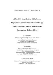
Bange, Barkauskas and Slater [1] defined a k-sequentially additive labeling f<br />
<strong>of</strong> a graph G(V, E) is a bijection from V ∪ E to {k, k+1, …, k+|V ∪ E|−1} such<br />
that for each edge xy, f(xy) = f(x) + f(y). If k =1, then G(V, E) is said to be<br />
1-sequentially additive graph or a simply sequentially additive graph or briefly, an<br />
SSA-graph. Figure 1 shows a graph with a 1-sequentially additive labeling.<br />
v2<br />
v6<br />
11<br />
9 7<br />
10 8<br />
1<br />
12 3 5<br />
2<br />
13 6<br />
Bange, Barkauskas, and slater [1] and Hedge and Miller [4] proved the<br />
following results.<br />
v1<br />
v3<br />
Fig. 1<br />
v5<br />
4<br />
v4
<strong>Simply</strong> sequentially additive labeling 6503<br />
Theorem 1.1 [1]: (i) Kn is 1-sequentially additive if and only if n ≤ 3; (ii) C3n+1 is<br />
not k-sequentially additive for k ≡ 0 or 2 (mod 3); (iii) C3n+2 is not k-sequentially<br />
additive for k ≡ 1 or 2 (mod 3).<br />
Theorem 1.2 [1]: The cycle Cn is 1-sequentially additive if and only if n ≡ 0, 1<br />
(mod 3).<br />
Theorem 1.3 [1]: The path Pn is 1-sequentially additive.<br />
Theorem 1.4 [1]: Given a graph G with V(G) = {v1, v2, …, vp} and r ≤ p, let H be<br />
the graph obtained from G by adding a new vertex vp+1 <strong>of</strong> degree r made adjacent<br />
to v1, v2, …, vr. If f is an SSA-numbering <strong>of</strong> G with f(vi) = i for 1 ≤ i ≤ r,<br />
then extending f by defining f(vp+1) = p+q+1 makes H simply sequentially<br />
additive.<br />
Theorem 1.5 [4]: Let Ca,b be a caterpillar with bipartition {A,B} where A = {u1,<br />
u2,…,ua} and B = {v1,v2,…,vb}, a ≤ b. Then Ca,b is k-sequentially additive for k =a<br />
and b.<br />
Theorem 1.6 [4]: K1,n is k-sequentially additive if and only if k divides n.<br />
Theorem 1.7 [4]: Denote a graph H = G(u,X) with V(H) = V(G) ∪ X and E(H) =<br />
E(G) ∪{ux : x ε X }, where u is a vertex <strong>of</strong> G and X is a new set <strong>of</strong> Vertices,<br />
disjoint from V(G). If G be a k-sequentially additive graph with a k-sequentially<br />
additive labeling f, then the graph H = G(u,X) with |X|= ar , where a = f(u) and r ≥<br />
1, is also a k-sequentially additive graph.<br />
Bange, Barkauskas, and slater [1] conjectured that all trees are 1-sequentially<br />
additive.<br />
In this paper we prove that the trees Bm,n, and related graphs,<br />
U n<br />
K1,<br />
i<br />
i=<br />
1<br />
, K1,n(1,2,…,n), the banana trees BT(n1, n2), BT(n, n, n) and BT(n, n, n, n)<br />
admit 1-sequentially additive labeling. The reader is directed to Harary [3] for all<br />
additional notation and terminology not provided in this paper.<br />
2 Main Results<br />
Now we provide the definitions for the graphs to be discussed in this paper.<br />
Bn,n is the n-bistar obtained from two disjoint copies <strong>of</strong> K1,n by joining the center<br />
vertices by an edge. Bm,n is the bistar obtained from two disjoint copies <strong>of</strong> K1,m<br />
and K1,n by joining the centre vertices by an edge. The tree is obtained<br />
from the bistar Bn,n by subdividing the edge joining the two stars. The graph B(r, s,<br />
t) is obtained from a path <strong>of</strong> length t by attaching the stars K1,r and K1,s with its<br />
pendent vertices.<br />
Next we define K1,n(1,2,…,n) is a graph obtained from K1,n <strong>of</strong> centre vertex v0<br />
and end vertices v1, v2, …, vn by joining i pendent vertices at each vi , i=1, 2,…, n.<br />
Throughout the paper we define the bijection f : V(G) ∪ E(G) → {1, 2, …,<br />
|V(G)|+ |E(G)|}. We denote the greatest integer less than or equal to the real<br />
number x by[ x ] .
6504 K. Manimekalai, J. Baskar Babujee and K. Thirusangu<br />
Theorem 2.1: The bistar Bm,n is 1-sequentially additive.<br />
Pro<strong>of</strong>: G(V,E) = Bm,n . Then G has (m+n+2) vertices and (m+n+1) edges. We<br />
define the bijection f : V ∪ E → {1, 2, …, 2(m+n)+3} as follows:<br />
Case 1: m or n or both m and n are even.<br />
Let n be even.<br />
Let V = V1 ∪ V2 ∪ V3, where V1 = {v1, v2}, V2 = {v1,i ; 1 ≤ i ≤ m},<br />
V3 = {v2,j ; 1≤ j ≤ n}with degree <strong>of</strong> v1 is (m+1) and degree <strong>of</strong> v2 is (n+1)<br />
and E = E1 ∪ E2 ∪ E3, where E1 = {v1v2}, E2 = {v1v1,i ; 1 ≤ i ≤ m},<br />
E3 = {v2v2,j ; 1 ≤ j ≤ n}.<br />
Define<br />
f(v1) = 1, f(v2) = 2, f(v1,i) = 2(i+1) ; 1 ≤ i ≤ m<br />
n<br />
⎧2(m<br />
+ 2j) ; 1 ≤ j ≤ 2<br />
f(v2,<br />
j)<br />
= ⎨<br />
n+<br />
2<br />
⎩2(m<br />
− n + 2j) + 1;<br />
2 ≤ j ≤ n<br />
f(v1 v2) = 3<br />
f(v1v1,i) = f(v1) + f(v1,i) = 2i +3 ; 1 ≤ i ≤ m<br />
⎧2(m<br />
+ 2j+<br />
1) ; 1≤<br />
j ≤<br />
f(v v ) = ⎨<br />
+<br />
⎩2(m<br />
− n + 2j) + 3 ; 2 ≤ j ≤ n.<br />
2 n<br />
n<br />
2<br />
2 2, j<br />
The labels are distinct and satisfy the condition f(uv) = f(u) + f(v) for each uv ∈ E.<br />
Hence Bm,n has 1-sequentially additive labeling, when m or n or both m, n are<br />
even.<br />
Case 2: Both m, n are odd.<br />
Subcase 2.1: n ≡ 0 (mod 3).<br />
Let V and E be defined as in case 1.<br />
Define<br />
f(v1) = 1, f(v2) = m+n+1,<br />
m-1<br />
⎧n<br />
+ 2i ; 1 ≤ i ≤ 2<br />
f(v1,<br />
i ) = ⎨<br />
m+<br />
1<br />
⎩2(n<br />
+ i + 1)<br />
; 2 ≤ i ≤ m<br />
f(v2,j) = j+1 ; 1 ≤ j ≤ n.<br />
f(v1 v2) = 3<br />
m-1<br />
⎧n<br />
+ 1+<br />
2i ; 1 ≤ i ≤ 2<br />
f(v1<br />
v1,<br />
i ) = ⎨<br />
m+<br />
1<br />
⎩2(n<br />
+ i) + 3 ; 2 ≤ i ≤ m<br />
f(v2v2,j) = (m+n+2) + j; 1 ≤ j ≤ n.<br />
The labels are distinct and satisfy the conditions f(uv) = f(u) + f(v) for each edge<br />
uv ∈ E. Hence the bistar Bm,n admits 1-sequentially additive labeling, when n is<br />
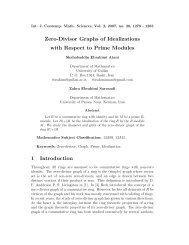
odd and n ≡ 0 (mod 3). In Fig. 2 we give the 1-sequentially additive labeling for<br />
the bistar B3,3.<br />
v1,2<br />
12<br />
5<br />
v1,3<br />
v1,1<br />
14<br />
13<br />
6<br />
15<br />
v1 8<br />
v2<br />
1 7<br />
Fig. 2: B3,3<br />
9<br />
10<br />
11<br />
v2,1<br />
2<br />
v2,3 4<br />
3<br />
v2,2
<strong>Simply</strong> sequentially additive labeling 6505<br />
Subcase 2.2: n ≡ 1 (mod 3).<br />
Let V = V1 ∪ V2 ∪ V3 ∪ V4, where<br />
n− 1<br />
V1 = {v1, v2}, V2 = {v1,i ; 1 ≤ i ≤ m}, V3 = {uk,j ; 1 ≤ k ≤ 3 and 1 ≤ j ≤ 3}<br />
n+ 2<br />
V4 = {uk,1 ; k = 3 } and E = E1 ∪ E2 ∪ E3 ∪ E4, where E1 = {v1v2},<br />
n− 1<br />
E2 = {v1v1,i ; 1 ≤ i ≤ m}, E3 = {v2uk,j ; 1 ≤ k ≤ 3 , 1 ≤ j ≤ 3}and<br />
n+ 2<br />
E4 = {v2uk,j ; k = 3 }.<br />
Define<br />
f(v1) = 1, f(v2) = 3, f(v1,i) = 2(n+i+1);1 ≤ i ≤ m,<br />
n-1<br />
⎧6k<br />
+ j −1<br />
; 1 ≤ k ≤ 3 & 1 ≤ j ≤ 3<br />
f(u k, j)<br />
= ⎨<br />
n+<br />
2<br />
⎩2<br />
; k = 3 & j = 1<br />
f(v1v2) = 4, f(v1v1,i) = 2(n+i)+3 ;1 ≤ i ≤ m,<br />
n-1<br />
⎧6k<br />
+ j+<br />
2 ; 1 ≤ k ≤ 3 & 1 ≤ j ≤ 3<br />
f(v2<br />
u k, j)<br />
= ⎨<br />
n+<br />
2<br />
⎩5<br />
; k = 3 & j = 1<br />
The labels are distinct and satisfy the conditions f(uv) = f(u) + f(v) for each edge<br />
uv ∈ E. Hence Bm,n admits 1-sequentially additive labeling, when m, n are odd<br />
and n ≡ 1 (mod 3).<br />
Subcase 2.3: n ≡ 2 (mod 3).<br />
Let V and E be defined as in case 1.<br />
Define<br />
f(v1) = m+n+1, f(v2) = 1, f(v1,i) = i+1 ; 1 ≤ i ≤ m,<br />
n-1<br />
⎧m<br />
+ 2j ; 1 ≤ j ≤ 2<br />
f(v2,<br />
j)<br />
= ⎨<br />
n+<br />
1<br />
⎩2(m<br />
+ j + 1) ; 2 ≤ j ≤ n<br />
f(v1v2) = m+n+2, f(v1v1,i)= (m+n+2) + i; 1 ≤ i ≤ m,<br />
n-1<br />
⎧m<br />
+ 2j + 1;<br />
1 ≤ j ≤ 2<br />
f(v 2v<br />
2, j)<br />
= ⎨<br />
n+<br />
1<br />
⎩2(m<br />
+ j) + 3 ; 2 ≤ j ≤ n<br />
The labels are distinct and satisfy the conditions f(uv) = f(u) + f(v) for each edge<br />
uv ∈ E. Hence the bistar Bm,n admits 1-sequentially additive labeling m, n are<br />
odd and n≡2 (mod 3).<br />
In all the cases Bm,n has a 1-sequentially additive labeling. Hence Bm,n is<br />
1-sequentially additive.<br />
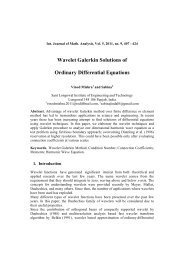
In Fig. 3 , we give the 1-sequentially additive labeling for the bistar B7,11.<br />
2<br />
11 v2,2<br />
v2,1<br />
3 v1,2 v1,1<br />
13 v2,3<br />
9<br />
12 v2,4<br />
4 v1,3 22 21<br />
10 15<br />
14<br />
23<br />
16 17 v2,5<br />
v1,4 24 v1 20 v2 18 28<br />
v2,6<br />
5<br />
19 1 29 30<br />
25<br />
31<br />
v1,5<br />
39 33 v2,7<br />
6 26<br />
32<br />
27<br />
37 35<br />
34 v2,8<br />
v1,6 7<br />
38<br />
v1,7 v2,11 36 v2,9<br />
8<br />
v2,10<br />
Fig. 3: B7,11
6506 K. Manimekalai, J. Baskar Babujee and K. Thirusangu<br />
In the following theorem we prove is a 1-sequentially additive<br />
graph.<br />
Theorem 2.2: The tree is 1-sequentially additive.<br />
Pro<strong>of</strong>: Let V be the vertex set and E be the edge set <strong>of</strong> . Then |V| =<br />
2n+3, |E| = 2n+2. We define bijection f : V ∪ E → {1, 2, …, 4n+5} as follows.<br />
Case 1: n is even.<br />
Let V = V1 ∪ V2 ∪ V3 , where V1 = {v1, v2, u0}, V2 = {v1,i ; 1 ≤ i ≤ n},<br />
V3 = {v2,j ; 1 ≤ j ≤ n}, deg (v1) = dev(v2) = n+1 and deg(u0) = 2 and all the other<br />
vertices are <strong>of</strong> degree one and E = E1 ∪ E2 ∪ E3, where E1 = {v1u0, v2u0}, E2 =<br />
{v1v1,i ; 1 ≤ i ≤ n}, E3 = {v2v2,j ; 1 ≤ j ≤ n}.<br />
Define<br />
f(v1) = 1, f(v2) = 2, f(u0) = 3, f(v1,i) = 2(i+2) ; 1 ≤ i ≤ n,<br />
n<br />
⎧2(n<br />
+ 2j+<br />
1) ; 1≤<br />
j ≤ 2<br />
f(v2,<br />
j)<br />
= ⎨<br />
n<br />
⎩3<br />
+ 4j;<br />
( 2 + 1)<br />
≤ j ≤ n<br />
f(v1u0) = 4, f(v2u0) = 5,<br />
f(v1v1,i) = 2i +5 ; 1 ≤ i ≤ n,<br />
n<br />
⎧2(n<br />
+ 2j + 2) ; 1 ≤ j ≤ 2<br />
f(v 2 v 2, j)<br />
= ⎨<br />
n<br />
⎩4j<br />
+ 5;<br />
( + 1)<br />
2 ≤ j ≤ n<br />
Case 2: n is odd.<br />
Subcase 2.1: n ≡ 0 (mod 3)<br />
Let V = V1 ∪ V2 ∪ V3 ∪ V4, where V1 = {v1, v2, u0}, V2 = {v1,i ; 1 ≤ i ≤ n},<br />
n n<br />
V3 = {ui,j ; 1 ≤ i ≤ [] 6 & 1 ≤ j ≤ 6}, V4 = {ui,j ; i = [ 6 ] + 1 & 1 ≤ j ≤ 3} and<br />
E = E1 ∪ E2 ∪ E3 ∪ E4 where E1 = {v1u0, v2u0}, E2 = {v1v1,i ; 1 ≤ i ≤ n},<br />
n n<br />
E3 = {v2ui,j ; 1 ≤ i ≤ [] 6 & 1 ≤ j ≤ 6}and E4 = {v2ui,j ; i =[ 6 ] +1 & 1 ≤ j ≤ 3}.<br />
Define<br />
f(v1) = 1, f(u0) = 4, f(v2) = 6,<br />
⎧2<br />
; i = 1<br />
⎪<br />
f(v1, i ) = ⎨11;<br />
i = 2<br />
⎪<br />
⎩2(n<br />
+ i + 2) ; 3 ≤ i ≤ n<br />
n<br />
⎧12i<br />
+ j+<br />
3 ; 1≤<br />
i ≤ [] 6 & 1≤<br />
j ≤ 6<br />
f(u i, j)<br />
= ⎨<br />
n<br />
⎩j<br />
+ 6 ; i = [] 6 + 1 & 1≤<br />
j ≤ 3<br />
f(v1u0) = 5, f(v2u0) = 10,<br />
⎧3<br />
; i = 1<br />
⎪<br />
f(v1 v1,<br />
i ) = ⎨12<br />
; i = 2<br />
⎪<br />
⎩2(n<br />
+ i) + 5 ; 3 ≤ i ≤ n<br />
n<br />
f(v2ui,j) = 12i +j + 9 ; 1≤ i ≤ [] 6 & 1 ≤ j ≤ 6<br />
f(v2ui,j) = j + 12 ; i = []<br />
6<br />
n +1 & 1 ≤ j ≤ 3.<br />
Subcase 2.2: (i) n ≡ 1 (mod 3) and n ≠1.<br />
Let V and E be defined as in case 1.
<strong>Simply</strong> sequentially additive labeling 6507<br />
We define f on V ∪ E as follows:<br />
f(v1) = 1, f(u0) = n+3, f(v2) = n+5,<br />
n+<br />
1<br />
⎧2i<br />
; 1≤<br />
i ≤ 2<br />
⎪<br />
n+<br />
3<br />
⎪<br />
n + 6 ; i = 2<br />
n+<br />
5<br />
f(v1,i<br />
) = ⎨2n<br />
+ 9 ; i = 2<br />
⎪<br />
n+<br />
7<br />
2n + 11;<br />
i = 2<br />
⎪<br />
n+<br />
9<br />
⎪⎩<br />
2(n + i + 2) ; 2 ≤ i ≤ n<br />
f(v2,j) = n+j+7 ; 1 ≤ j ≤ n<br />
n+<br />
1<br />
⎧2i<br />
+ 1`;<br />
1 ≤ i ≤ 2<br />
⎪<br />
n+<br />
3<br />
⎪<br />
n + 7 ; i = 2<br />
n+<br />
5<br />
f(v1u0) = n+ 4, f(v2u0) = 2n + 8, f(v1<br />
v1,<br />
i ) = ⎨2n<br />
+ 10 ; i = 2<br />
⎪<br />
n+<br />
7<br />
2n + 12 ; i = 2<br />
⎪<br />
n+<br />
9<br />
⎪⎩<br />
2(n + i) + 5 ; 2 ≤ i ≤ n<br />
f(v2,v2,j) = 2n+12 +j ; 1 ≤ j ≤ n.<br />
(ii). If n =1, then is a Path P5. By Theorem 1.3[1], it is an SSA-graph.<br />
Subcase 2.3: n ≡ 2 (mod 3).<br />
Let V and E be defined as in case 1.<br />
Define f on V ∪ E as follows:<br />
n+<br />
1<br />
⎧2i<br />
; 1 ≤ i ≤ 2<br />
⎪<br />
n+<br />
3<br />
⎪2(n<br />
+ 3) ; i = 2<br />
f(v1) = 1, f(v2) = n+5, f(u0) = n+3, f(v1,<br />
i ) = ⎨<br />
n+<br />
5<br />
⎪2n<br />
+ 9 ; i = 2<br />
⎪<br />
n+<br />
7<br />
⎩2(n<br />
+ 2 + i) ; 2 ≤ i ≤ n<br />
f(v2,j) = n+5+j ; 1 ≤ j ≤ n.<br />
f(v1u0) = n+ 4, f(v2u0) = 2n + 8<br />
n+<br />
1<br />
⎧2i<br />
+ 1;<br />
1 ≤ i ≤ 2<br />
⎪<br />
n+<br />
3<br />
⎪2n<br />
+ 7 ; i = 2<br />
f(v1<br />
v1,<br />
i ) = ⎨<br />
n+<br />
5<br />
⎪2n<br />
+ 10 ; i = 2<br />
⎪<br />
n+<br />
7<br />
⎩2(n<br />
+ i) + 5 ; 2 ≤ i ≤ n<br />
f(v2v2,j) = 2n+10 +j ; 1 ≤ j ≤ n.<br />
In all the above cases, the labels are distinct and satisfy the condition f(uv) = f(u)<br />
+ f(v) for each uv ∈ E. Hence admits 1-sequentially additive labeling.<br />
In Fig. 4, we display 1-sequentially additive labeling for .
6508 K. Manimekalai, J. Baskar Babujee and K. Thirusangu<br />
v1,3<br />
6<br />
4<br />
v1,4<br />
7<br />
16<br />
v1,2<br />
17<br />
5<br />
v1<br />
2 11<br />
3<br />
v1,1<br />
9 u0<br />
1 8<br />
20<br />
19<br />
v1,5<br />
Fig. 4: <br />
Remark 2.1: It follows from the Theorem 1.5[4], is a 2- sequentially<br />
additive and as well as (2n+1) - sequentially additive graph.<br />
Theorem 2.3: Let G(V,E) be the graph obtained from the tree by<br />
appending two pendent edges to a new vertex which subdivides the edge joining<br />
the centre vertices <strong>of</strong> the two copies <strong>of</strong> k1,n in . Then G is an SSA graph.<br />
Pro<strong>of</strong>: The graph G has 2n+5 vertices and 2n+4 edges. We define a map f : V ∪<br />
E → {1, 2, …, 4n+9} as follows:<br />
Case 1: n is even.<br />
Let the vertex set V(G) = V1 ∪ V2 ∪ V3 , where V1 = {wi : 0 ≤ i ≤ 4 }, V2 =<br />
{ui ; 1 ≤ i ≤ n}, V3 = {vi : 1 ≤ i ≤ n } and the edge set E(G) = E1 ∪ E2 ∪ E3 , where<br />
E1 = {w0wi : 1 ≤ i ≤ 4 }, E2 = {w1ui : 1 ≤ i ≤ n }, E3 = {w2vi : 1 ≤ i ≤ n }.<br />
Define<br />
f(w0) = 5, f(wi) = i, 1 ≤ i ≤ 4<br />
f(ui) = 2(i+4) ; 1 ≤ i ≤ n<br />
n<br />
⎧2(n<br />
+ 2i + 3) ; 1 ≤ i ≤ 2<br />
f(vi<br />
) = ⎨<br />
n<br />
⎩4i<br />
+ 7 ; ( 2 + 1)<br />
≤ i ≤ n<br />
f(w0wi) = 5+i ; 1 ≤ i ≤ 4<br />
f(w1ui) = 2i+9 ; 1 ≤ i ≤ n<br />
n<br />
⎧2(n<br />
+ 2i + 4) ; 1 ≤ i ≤ 2<br />
f(w 2 vi<br />
) = ⎨<br />
n<br />
⎩4i<br />
+ 9;<br />
( 2 + 1)<br />
≤ i ≤ n<br />
Case 2: n is odd.<br />
Subcase 2.1: n ≡ 0 (mod 3)<br />
Let V(G) = V1 ∪ V2 ∪ V3 and E(G) = E1 ∪ E2 ∪ E3 , where V1, V2 , E1 and E2 are<br />
n as defined in case 1 and V3 = {vk,j ; 1≤ k ≤ 3 , 1 ≤ j ≤ 3},<br />
n<br />
E3 = {w2vk,j ; 1≤ k ≤ 3 & 1 ≤ j ≤ 3}.<br />
f(w1) = 1, f(w2) = 3, f(w3) = 2, f(w4) = 4, f(w0) = 5<br />
f(ui) = 2(i+4) ; 1 ≤ i ≤ n<br />
n<br />
f(vk,j) = 2n+6k+j+3 ; 1 ≤ k ≤ 3 , 1≤ j ≤ 3<br />
f(w0w1) = 6, f(w0w2) =8, f(w0w3) = 7, f(w0w4) = 9<br />
18<br />
15<br />
v2,1<br />
21<br />
v2<br />
10<br />
25<br />
v2,5<br />
12<br />
22<br />
23<br />
24<br />
14<br />
v2,2<br />
v2,4<br />
v2,3<br />
13
<strong>Simply</strong> sequentially additive labeling 6509<br />
f(w1ui) = 2i+9 ; 1 ≤ i ≤ n<br />
n<br />
f(w2vk,j) = 2n+6k+j+6 ; 1 ≤ k ≤ 3 , 1≤ j ≤ 3<br />
Subcase 2.2: n ≡ 1 (mod 3)<br />
Let V(G) = V1 ∪ V2 ∪ V3 ∪ V4 , where V1 = {wi ; 0 ≤ i ≤ n}, V2 = {ui ; 1 ≤ i ≤ n} ,<br />
n<br />
V3 = {vk,j ; 1 ≤ k ≤ [] 3<br />
, 1 ≤ j ≤ 3}, V4 = {vk,1 ; k = 3<br />
and E(G) = E1 ∪ E2 ∪ E3 ∪ E4 , where<br />
E1 = {w0wi ; 1 ≤ i ≤ 4 } , E2 ={w1ui ; 1 ≤ i ≤ n } ,<br />
E3 ={w2vk,j ; 1 ≤ k ≤ []<br />
3<br />
n+ 2 }<br />
n , 1 ≤ j ≤ 3 } and E4 = {w2vk,1 ; k = 3<br />
For 0 ≤ i ≤ 4, assign the label to wi and w0wi as in subcase 2.1.<br />
⎧11<br />
f(ui ) = ⎨<br />
⎩2(i<br />
+ 5)<br />
;<br />
;<br />
i = 1<br />
2 ≤ i ≤ n<br />
⎧2n<br />
+ 6k + j + 5 ;<br />
f(vk,<br />
j)<br />
= ⎨<br />
⎩10;<br />
For 0 ≤ i ≤ 4<br />
n-1<br />
1 ≤ k ≤ 3 ; 1 ≤ j ≤ 3<br />
n+<br />
2 k = 3 ; j = 1<br />
⎧12<br />
;<br />
f(w1 u i ) = ⎨<br />
⎩ 2i + 11 ;<br />
i = 1<br />
2 ≤ i ≤ n<br />
⎧2n<br />
+ 6k + j + 8 ;<br />
f(w 2v<br />
k, j)<br />
= ⎨<br />
⎩13;<br />
n-1<br />
1 ≤ k ≤ 3<br />
n+<br />
2 k = 3<br />
; 1 ≤ j ≤ 3<br />
; j = 1<br />
Subcase 2.3: n ≡ 2 (mod 3)<br />
Let V(G) and E(G) be defined as in case 1.<br />
f(w0) = n+3 ,f(w1) = 1, f(w2) = n + 5 , f(w3) = 4 , f(w4) = 5<br />
⎧2<br />
; i = 1<br />
⎪<br />
⎪<br />
2(i + 1) ; 2 ≤ i ≤<br />
+<br />
f(u ) = ⎨2n<br />
+ 9 ; i =<br />
⎪<br />
+<br />
2n + 12; i = 2 ⎪<br />
⎩(5n<br />
+ 2i + 21) 2 ;<br />
3 n<br />
2 1 n<br />
i<br />
f(w0w1) = n + 4 , f(w0w2) = 2n+8,<br />
f(w0w3) = n + 7 , f(w0w4) = n + 8 ,<br />
f(w 2 i<br />
⎧2n<br />
+ 11<br />
v ) = ⎨<br />
⎩2n<br />
+ i + 12<br />
;<br />
;<br />
2 1 - n<br />
n+<br />
5<br />
2<br />
⎧3<br />
; i = 1<br />
⎪<br />
⎪<br />
2i + 3 ; 2 ≤ i ≤<br />
f(w u ) = ⎨2n<br />
+ 10 ; i =<br />
⎪<br />
+<br />
2n + 13;<br />
i =<br />
⎪<br />
⎩(5n<br />
+ 2i + 23) 2 ;<br />
n<br />
n<br />
1<br />
i<br />
+<br />
2 1<br />
2 1 - n<br />
≤ i ≤ n<br />
2<br />
n+<br />
5<br />
2<br />
3<br />
≤ i ≤ n<br />
i = 1<br />
2 ≤ i ≤ n<br />
)<br />
f(v i<br />
⎧n<br />
+ 6<br />
= ⎨<br />
⎩n<br />
+ i + 7<br />
n+ 2 }<br />
;<br />
;<br />
i = 1<br />
2 ≤ i ≤ n
6510 K. Manimekalai, J. Baskar Babujee and K. Thirusangu<br />
In all the above cases, the labels are distinct and satisfy the condition f(uv) =f(u)<br />
+f(v) for each uv Є E. Hence G admits an 1-sequentially additive labeling.<br />
SSA-labeling <strong>of</strong> the graph G in Theorem 2.3 with n= 6 is given in Fig. 5.<br />
12<br />
14 15<br />
16<br />
We denote by<br />
Un K1,<br />
i<br />
i=<br />
1<br />
Theorem 2.4: The graph U n<br />
the union <strong>of</strong> n disjoint copies <strong>of</strong> K1,i for i = 1, 2, …, n.<br />
K1,<br />
i<br />
i=<br />
1<br />
is an SSA graph.<br />
Pro<strong>of</strong>. Let V be the vertex set and E be the edge set <strong>of</strong> K . Then |V|+|E| = n 2 +<br />
2n. V and E be defined as V = {vi,j ; 1 ≤ i ≤ n and 1 ≤ j ≤ i} ∪ {vi ; 1 ≤ i ≤ n}, E =<br />
{vivi,j ; 1 ≤ i ≤ n and 1 ≤ j ≤ i}. We define the bijection f : V ∪ E → {1, 2, …<br />
n 2 +2n} as follows.<br />
f(vi) = i; 1 ≤ i ≤ n, f(vi,j) = n + i 2 − i + j for 1 ≤ i ≤ n and 1 ≤ j ≤ i, f(vivi,j) = n + i 2<br />
+ j for 1 ≤ i ≤ n and 1 ≤ j ≤ i. Therefore the labels are distinct and satisfy the<br />
condition f(uv) = f(u) + f(v) for each edge uv ∈ E. Hence U n<br />
n<br />
U<br />
i=<br />
1<br />
1, i<br />
K1,<br />
i<br />
i=<br />
1<br />
is an<br />
SSA-graph.<br />
The graph K1,n(1,2,…,n) which we defined earlier is the same as the graph<br />
obtained from U n<br />
13<br />
17<br />
i=<br />
1<br />
18<br />
K<br />
19<br />
1, i<br />
11<br />
1<br />
10<br />
21<br />
6<br />
20<br />
by joining the centre vertex vi <strong>of</strong> each K1,i (i = 1, 2, …, n)<br />
by an edge to a new vertex v0.<br />
By Theorem 1.4 [1] and Theorem 2.4, we have the following the corollary.<br />
Corollary 2.5: The graph K1,n(1,2,…,n) is an SSA-graph.<br />
Pro<strong>of</strong>: The labeling f defined onU n<br />
i=<br />
1<br />
K<br />
1, i<br />
3<br />
8<br />
9<br />
4<br />
5<br />
Fig. 5<br />
in theorem 3.2 is extended to the vertex v0<br />
and the edges adjacent to v0 by f(v0) = (n+1) 2 and f(v0vi) = (n+1) 2 + i for 1≤ i ≤n,<br />
we have K1,n(1,2,…,n) is an SSA-graph.<br />
7<br />
22<br />
31<br />
33<br />
24<br />
2<br />
29<br />
28<br />
26<br />
32<br />
25<br />
27<br />
30
<strong>Simply</strong> sequentially additive labeling 6511<br />
SSA-labeling <strong>of</strong> the graph K1,n(1,2,…,n) in Corollary 2.5 with n= 5 is shown in<br />
Figure 6.<br />
30<br />
29<br />
28<br />
27<br />
26<br />
35<br />
34<br />
33<br />
32<br />
31<br />
In the following theorems, we present an SSA-labeling <strong>of</strong> some particular<br />
types <strong>of</strong> banana trees. The banana tree is defined as follows.<br />
K , K ,..., K be a family <strong>of</strong> disjoint stars with the vertex sets<br />
Let 1, n1<br />
1, n2<br />
1, nk<br />
V(K n ) i {ci<br />
, vi,1,...,<br />
vi,<br />
ni<br />
21<br />
v5<br />
5<br />
25<br />
4<br />
20<br />
41<br />
24<br />
v4<br />
19<br />
40<br />
22<br />
23<br />
18<br />
v0<br />
36<br />
1, = } and deg(ci) = ni, 1 ≤ i ≤ k. A banana tree BT(n1, n2, …,<br />
nk) is a tree obtained by adding a new vertex and joining it to v1,1, v2,1, …, vk,1.<br />
Denote the vertex and edge sets <strong>of</strong> G(V,E) ≅ BT(n1, n2, …, nk) as follows:<br />
V(G) = {v} ∪ {ci ; 1 ≤ i ≤ k} ∪ {vi,j ; 1 ≤ i ≤ k, 1 ≤ j ≤ ni} and<br />
E(G) = {vvi,1 ; 1 ≤ i ≤ k} ∪ {civi,j ; 1 ≤ i ≤ k, 1 ≤ j ≤ ni}.<br />
Theorem 2.6: The banana tree BT(n1, n2) admits an SSA-labeling.<br />
Pro<strong>of</strong>: Let G = BT(n1, n2).We consider two cases.<br />
Case 1: n1 ≥ n2 > 1<br />
V(G) = {v, c1, c2} ∪ {vi,j ; 1 ≤ i ≤ 2, 1 ≤ j ≤ ni}<br />
E(G) = {vvi,1;1 ≤ i ≤ 2} ∪ {civi,j ; 1 ≤ i ≤ 2, 1 ≤ j ≤ ni}<br />
Then |V(G)| = n1 + n2 + 3 and |E(G)| = n1 + n2 + 2.<br />
Define a labeling f : V ∪ E → {1, 2, …, 2(n1+n2) + 5} as follows:<br />
For 1 ≤ i ≤ 2<br />
f(v) = 2, f(ci) = 2i−1<br />
f(vi,1) = 3i+1<br />
f(vi,2) = 4(4−i)<br />
f(vi,j) = 4j−i+4, 3 ≤ j ≤ n2<br />
f(v1,j) = 2(n2+j+2); n2+1 ≤ j ≤ n1<br />
f(vvi,1) = 3(i+1)<br />
⎪<br />
⎧5i;<br />
j = 1<br />
f(ci<br />
vi,<br />
j)<br />
= ⎨15<br />
− 2i; j = 2<br />
⎪⎩ i + 4j + 3; 3 ≤ j ≤ n 2.<br />
f(c1v1,j) = 2n2 + 2j + 5; n2 + 1 ≤ j ≤ n1.<br />
The labels defined above are all distinct and satisfy the condition f(uv) = f(u) + f(v)<br />
for each uv ∈ E(G) and for n1 ≥ n2 > 1.<br />
17<br />
14<br />
39<br />
v3<br />
Fig. 6<br />
3<br />
15<br />
16<br />
13<br />
38<br />
12<br />
37<br />
v2<br />
11<br />
9<br />
2<br />
10<br />
8<br />
1<br />
6<br />
v1<br />
7
6512 K. Manimekalai, J. Baskar Babujee and K. Thirusangu<br />
Case 2. n1 ≥ n2 = 1. Then V(G) = {v} ∪ {c1, c2} ∪ {v1,j ; 1 ≤ j ≤ n1} ∪{v2,1} and<br />
E(G) = {vv1,1, vv2,1} ∪ c2v2,1} ∪ {c1v1,j ; 1 ≤ j ≤ n1}<br />
and |V(G) ∪ E(G)| = 2n1 + 7.<br />
We define the labeling f : V(G) ∪ E(G) → {1, 2, …, 2n1+7} as follows:<br />
f(ci) = i, i = 1, 2; f(v) = 3,<br />
f(vi,1) = 2(i+1); i = 1, 2;<br />
f(v1,j) = 6+2j; 2 ≤ j ≤ n1.<br />
f(vvi,1) = 2i+5; i = 1, 2<br />
f(civi,1) = 3i+2; i = 1, 2<br />
f(c1v1,j) = 2j+7; 2 ≤ j ≤ n1<br />
In both cases, the labels defined on V(G) ∪ E(G) are all distinct and satisfy the<br />
condition f(uv) = f(u) + f(v) for each uv ∈ E(G). Hence the graph BT(n1, n2)<br />
admits an SSA-labeling.<br />
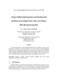
An SSA-labeling <strong>of</strong> BT(6, 6) is shown in Figure 7.<br />
27<br />
23<br />
19<br />
15<br />
20 16<br />
24 13<br />
21 17 11<br />
5<br />
25 10<br />
28 29<br />
1<br />
12<br />
4<br />
Fig. 7: SSA – labeling <strong>of</strong> BT(6,6)<br />
Theorem 2.7: The banana tree BT(n, n, n) admits an SSA-labeling.<br />
Pro<strong>of</strong>: Let G = BT(n, n, n) and the vertex and edge sets <strong>of</strong> G be V(G) = {v} ∪<br />
{ci / 1 ≤ i ≤ 3} ∪ {vi,j / 1 ≤ i ≤ 3, 1 ≤ j ≤ n} and E(G) = {vvi,1} ∪ {civi,j / 1 ≤ i ≤ 3,<br />
1 ≤ j ≤ n} respectively. Then |V(G) ∪ E(G)| = 6n+7. Define a labeling f : V ∪ E<br />
→ {1, 2, ..., 6n+7} as follows:<br />
f(v) = 1; f(ci) = i+1; 1 ≤ i ≤ 3<br />
f(v1,1) = 11, f(v2,1) = 7, f(v3,1) = 5<br />
For 2 ≤ j ≤ n<br />
f(v1,j) = 6j+3, f(v2,j) = 6j+4, f(v3,j) = 6j+2<br />
f(vv1,1) = 12, f(vv2,1) = 8, f(vv3,1) = 6<br />
f(c1v11) = 13, f(c2v21) = 10, f(c3v3,1) = 9<br />
For 2 ≤ j ≤ n<br />
f(c1v1,j) = 6j+5, f(c2v2,j) = 6j+7, f(c3v3,j) = 6j+6.<br />
Clearly the labels defined above are distinct and satisfy the condition f(uv) = f(u)<br />
+ f(v) for each uv ∈ E(G). Hence G ≅ BT(n, n, n) is an SSA-graph.<br />
SSA-labeling <strong>of</strong> BT(7, 7, 7) is shown in Figure 8.<br />
26<br />
6<br />
22<br />
2<br />
18<br />
3<br />
14<br />
9<br />
8<br />
7
<strong>Simply</strong> sequentially additive labeling 6513<br />
45 39 33 27 21 15 11 46 40 34 28 22 16 7 44 38 32 26 20 14<br />
2<br />
Fig. 8: SSA – labeling <strong>of</strong> BT(7,7,7)<br />
Theorem 2.8: The banana tree BT(n, n, n, n) is an SSA-graph.<br />
Pro<strong>of</strong>: Let G(V,E) = BT(n, n, n, n) and V(G) = {v} ∪ {ci / 1 ≤ i ≤ 4} ∪ {vi,j / 1 ≤ i<br />
≤ 3, 1 ≤ j ≤ n} and E(G) = {vvi,1} ∪ {civi,j / 1 ≤ i ≤ 4, 1 ≤ j ≤ n} respectively. Then<br />
|V(G) ∪ E(G)| = 8n+9. Then |V(G) ∪ E(G)| = 8n+9. We define a bijection f : V(G)<br />
∪ E(G) → {1, 2, …, 8n+9} as follows:<br />
Case 1: n ≥ 2.<br />
For the vertices<br />
f(v) = 1, f(ci) = i+1; 1 ≤ i ≤ 4.<br />
f(v1,1) = 17, f(v2,1) = 13, f(v3,1) = 8, f(v4,1) = 6<br />
f(v1,2) = 21, f(v2,2) = 22, f(v3,2) = 20, f(v4,2) = 10<br />
f(v1,j) = 8j+6; 3 ≤ j ≤ n.<br />
f(vi,j) = i+8j; 2 ≤ i ≤ 4, 3 ≤ j ≤ n.<br />
f(vv1,1) = 18, f(vv2,1) = 14, f(vv3,1) = 9, f(vv4,1) = 7<br />
f(c1v1,1) = 19, f(c2v2,1) = 16, f(c3v3,1) = 12, f(c4v4,1) = 11<br />
f(c1v1,2) = 23, f(c2,v2,2) = 25, f(c3v3,2) = 24, f(c4v4,2) = 15<br />
f(c1v1,j) = 8(j+1); 3 ≤ j ≤ n<br />
f(civi,j) = 2i+8j+1; 2 ≤ i ≤ 4, 3 ≤ j ≤ n<br />
Clearly the labels defined on V ∪ E satisfy the condition f(uv) = f(u) + f(v) for<br />
each uv ∈ E(G).<br />
Case 2: Let n = 1. An SSA-labeling <strong>of</strong> BT(1,1,1,1) is shown in Figure 9.<br />
2<br />
8<br />
6<br />
14 9<br />
3 4<br />
17<br />
13<br />
7<br />
Thus in both cases BT(n, n, n, n) admits an SSA-labeling.<br />
15<br />
1<br />
3<br />
10<br />
12<br />
Fig. 9: BT(1,1,1,1)<br />
11<br />
16<br />
1<br />
5<br />
4<br />
5
6514 K. Manimekalai, J. Baskar Babujee and K. Thirusangu<br />
For example, SSA-labeling <strong>of</strong> B(6, 6, 6, 6) is shown in Fig.10.<br />
21<br />
References<br />
17<br />
30 19<br />
23<br />
38 32<br />
40<br />
46 48<br />
54<br />
56<br />
42<br />
50<br />
[1] D.W. Bange, A.E. Barkauskas and P.J. Slater, <strong>Sequentially</strong> additive graphs,<br />
Discrete Math., 44 (1983), 235−241.<br />
[2] J.A. Gallian, A Dynamic Survey <strong>of</strong> Graph <strong>Labeling</strong>, Electronic Journal <strong>of</strong><br />
Combinatorics, 17 (2010), # DS6.<br />
[3] F.Harary, Graphy Theory, Addison Wesley, Reading, Massachusetts, 1969.<br />
[4] S.M. Hegde and M. Miller, Further results on sequentially additive graphs,<br />
Discussiones Mathematicae Graph Theory, 27 (2007), 251−268.<br />
Received: August, 2012<br />
34<br />
29<br />
45<br />
37 25 16<br />
53<br />
2<br />
26<br />
3<br />
22<br />
13<br />
43 35 27<br />
20<br />
51<br />
47 39 31 24 12<br />
55<br />
8<br />
52<br />
44<br />
36<br />
57 49<br />
41<br />
33<br />
28<br />
4<br />
15 10<br />
5<br />
11<br />
6<br />
Fig. 10: SSA-labeling <strong>of</strong> BT(6,6,6,6)<br />
1