Wavelet Galerkin Solutions of Ordinary Differential Equations
Wavelet Galerkin Solutions of Ordinary Differential Equations
Wavelet Galerkin Solutions of Ordinary Differential Equations

Create successful ePaper yourself
Turn your PDF publications into a flip-book with our unique Google optimized e-Paper software.
Int. Journal <strong>of</strong> Math. Analysis, Vol. 5, 2011, no. 9, 407 - 424<br />
<strong>Wavelet</strong> <strong>Galerkin</strong> <strong>Solutions</strong> <strong>of</strong><br />
<strong>Ordinary</strong> <strong>Differential</strong> <strong>Equations</strong><br />
Vinod Mishra 1 and Sabina 2<br />
Sant Longowal Institute <strong>of</strong> Engineering and Technology<br />
Longowal 148 106 Punjab, India<br />
1 vinodmishra.2011@rediffmail.com, 2 sabinajindal8@gmail.com<br />
Abstract. Advantage <strong>of</strong> wavelet <strong>Galerkin</strong> method over finite difference or element<br />
method has led to tremendous applications in science and engineering. In recent<br />
years there has been increasing attempt to find solutions <strong>of</strong> differential equations<br />
using wavelet techniques. In this paper, we elaborate the wavelet techniques and<br />
apply <strong>Galerkin</strong> procedure to analyse one dimensional harmonic wave equation as a<br />
test problem using fictitious boundary approach; overcoming Dianfeng et al. (1996)<br />
reservation at higher resolution. This could have been possible only after evaluating<br />
connection coefficients at various scales.<br />
Keywords. <strong>Wavelet</strong> <strong>Galerkin</strong> Method; Condition Number; Connection Coefficients;<br />
Moments; Harmonic Wave Equation.<br />
1. Introduction<br />
<strong>Wavelet</strong> functions have generated significant interest from both theoretical and<br />
applied research over the last few years. The name wavelet comes from the<br />
requirement that they should integrate to zero, waving above and below x-axis. The<br />
concepts for understanding wavelets were provided recently by Meyer, Mallat,<br />
Daubechies, and many others. Since then, the number <strong>of</strong> applications where wavelets<br />
have been used has exploded.<br />
Many different types <strong>of</strong> wavelet functions have been presented over the past few<br />
years. In this paper, the Daubechies family <strong>of</strong> wavelets will be considered due to<br />
their useful properties.<br />
Since the contribution <strong>of</strong> orthogonal bases <strong>of</strong> compactly supported wavelet by<br />
Daubechies (1988) and multiresolution analysis based fast wavelet transform<br />
algorithm by Belkin (1991), wavelet based approximation <strong>of</strong> ordinary differential
408 V. Mishra and Sabina<br />
equations gained momentum in attractive way. <strong>Wavelet</strong>s have the capability <strong>of</strong><br />
representing the solutions at different levels <strong>of</strong> resolutions, which make them<br />
particularly useful for developing hierarchical solutions to engineering problems.<br />
Among the approximations, wavelet <strong>Galerkin</strong> technique is the most frequently used<br />
scheme these days. Daubechies wavelets as bases in a <strong>Galerkin</strong> method to solve<br />
differential equations require a computational domain <strong>of</strong> simple shape. This has<br />
become possible due to the remarkable work by Latto et al. [1], Xu et al. [4],<br />
Williams et al. [5 & 6] and Amartunga et al. [10]. Yet there is difficulty in dealing<br />
with boundary conditions. So far problems with periodic boundary conditions or<br />
periodic distribution have been dealt successfully. Fictitious boundary approach with<br />
Dirichlet boundaries has been applied by Dianfeng et al. [11] in analysing SH wave,<br />
but found difficulty near resonance response. In this paper, it is overcome by finding<br />
connection coefficients at different scales. Remind that Latto et al. [1] provides<br />
connection coefficients for j=0 and N=6 only. A detailed exposition <strong>of</strong> problem with<br />
distinct boundaries is also dealt by Jordi Besora [8].<br />
2<br />
<strong>Wavelet</strong> (x)<br />
: An oscillatory function ( x) L ( R)<br />
with zero mean is a wavelet if<br />
it has the desirable properties:<br />
1. Smoothness: (x)<br />
is n times differentiable and that their derivatives are<br />
continuous.<br />
2. Localization: (x)<br />
is well localized both in time and frequency domains, i.e.,<br />
(x)<br />
and its derivatives must decay very rapidly. For frequency localization ˆ<br />
( )<br />
must decay sufficiently fast as and that ˆ ( )<br />
becomes flat in the<br />
neighborhood <strong>of</strong> 0 . The flatness is associated with number <strong>of</strong> vanishing<br />
moments <strong>of</strong> (x)<br />
, i.e.<br />
<br />
x x dk<br />
<br />
k<br />
( ) =0 or equivalently ˆ<br />
( )<br />
0<br />
k<br />
k<br />
d<br />
for k 0,<br />
1,<br />
........., n<br />
d<br />
in the sense that larger the number <strong>of</strong> vanishing moments more is the flatness when<br />
is small.<br />
3. The admissibility condition<br />
<br />
<br />
<br />
ˆ<br />
( )<br />
<br />
suggests that<br />
2<br />
d<br />
<br />
2<br />
ˆ( )<br />
decays at least as<br />
1<br />
or<br />
1<br />
x for 0 .<br />
Daubechies <strong>Wavelet</strong>. Daubechies wavelets are compactly supported functions. This<br />
means that they have non zero values within a finite interval and have a zero value
<strong>Wavelet</strong> <strong>Galerkin</strong> solutions 409<br />
everywhere else. That’s why it is useful for representing the solution <strong>of</strong> differential<br />
equation. In 1988, Ingrid Daubechies defined scaling function as<br />
( x)<br />
N 1<br />
<br />
k0<br />
a (<br />
2x<br />
k),<br />
k<br />
where N denotes the genus <strong>of</strong> the Daubechies wavelet. The functions generated<br />
with these coefficients will have supp [ 0,<br />
N 1]<br />
and ( N / 2 1)<br />
vanishing wavelet<br />
moments.<br />
Sometimes the scaling functions are defined as<br />
N 1<br />
( x)<br />
2<br />
c ( 2x<br />
k),<br />
<br />
<br />
<br />
k0<br />
k<br />
where ak 2ck<br />
, with the property that N 1<br />
c k 2 .<br />
k0<br />
We have computed the Daubechies coefficients for N=4, 6, 8, 10, 12 in the Table<br />
given below:<br />
k<br />
N=4<br />
Table 1.1: Daubechies <strong>Wavelet</strong> Filter Coefficients c k<br />
N=6<br />
N=8<br />
N=10<br />
N=12<br />
N=14<br />
0 0.4830 0.3327 0.2304 0.1601 0.1115 0.0779<br />
N=16<br />
0.0544<br />
1 0.8365 0.8069 0.7148 0.6038 0.4946 0.3965 0.3129<br />
2 0.2241 0.4599 0.6309 0.7243 0.7511 0.7291 0.6756<br />
3 -0.1294 -0.1350 -0.0280 0.1384 0.3153 0.4698 0.5854<br />
4 -0.0854 -0.1870 -0.2423 -0.2263 -0.1439 -0.0158<br />
5 0.0352 0.0308 -0.0322 -0.1298 -0.2240 -0.2840<br />
6 0.0329 0.0776 0.0975 0.0713 0.0005<br />
7 -0.0106 -0.0062 0.0275 0.0806 0.1287<br />
8 -0.0126 -0.0316 -0.0380 -0.0174<br />
9 0.0033 0.0006 -0.0166 -0.0441<br />
10 0.0048 0.0126 0.0140<br />
11 -0.0011 0.0004 0.0087<br />
12 -0.0018 -0.0049<br />
13 0.0004 -0.0004<br />
14 0.0007<br />
15 -0.0001<br />
The associated wavelet function is given by
410 V. Mishra and Sabina<br />
1<br />
k<br />
( x)<br />
( 1)<br />
a1k<br />
( 2x<br />
k)<br />
.<br />
<br />
k 2<br />
N<br />
2. <strong>Wavelet</strong> <strong>Galerkin</strong> Technique<br />
<strong>Galerkin</strong> Method. It was Russian engineer V.I. <strong>Galerkin</strong> who proposed a projection<br />
method based on weak form. In it a set <strong>of</strong> test functions are selected such that<br />
residual <strong>of</strong> differential equation becomes orthogonal to test functions [8].<br />
Consider one-dimensional differential equation [12, pp. 451-479]<br />
Lu ( x)<br />
f ( x),<br />
0 x 1<br />
(2.1)<br />
with Dirichlet boundary conditions<br />
u( 0)<br />
a,<br />
u(<br />
1)<br />
b.<br />
f is real valued and continuous functions <strong>of</strong> x on [0,1]. L is a uniformly elliptic<br />
differential operator.<br />
L 2 ([0, 1]) is a Hilbert space with inner product<br />
<br />
Suppose that j <br />
is<br />
1<br />
f , g<br />
f ( x)<br />
g(<br />
x)<br />
dt.<br />
2<br />
C on [0, 1] such that<br />
v j 0)<br />
a,<br />
v j ( 1)<br />
<br />
0<br />
v is a complete orthonormal system for L 2 ([0, 1]) and that every j v<br />
( b.<br />
Select a finite set <strong>of</strong> indices j and consider the subspace<br />
S span v j : j <br />
<br />
Let the approximate solution u s <strong>of</strong> the given equation be<br />
us xk<br />
vk<br />
S.<br />
<br />
k<br />
(2.2)<br />
We would like to determine xk in a way that us behaves as if is a true solution on S,<br />
i.e.<br />
u , v f , v j <br />
(2.3)<br />
L s j<br />
j<br />
such that the boundary conditions u s ( 0)<br />
u s ( 1)<br />
0 are satisfied. Substituting u s in<br />
(2.3),<br />
v , v x<br />
f , v j .<br />
(2.4)<br />
<br />
k<br />
L k j k<br />
j<br />
Let X and Y denote the vectors x k and , ,<br />
k<br />
k f v<br />
k<br />
k<br />
A <br />
a j k j , k<br />
, , where a j,<br />
k Lv<br />
k , v j .<br />
(2.4) reduces to the system <strong>of</strong> linear equations<br />
y and A the matrix
<strong>Wavelet</strong> <strong>Galerkin</strong> solutions 411<br />
<br />
k<br />
a x y<br />
j,<br />
k k j or equivalently AX = Y . (2.5)<br />
Thus in <strong>Galerkin</strong> method, for each subset , we find an approximation u s in S to u<br />
by solving (2.5) for X and then substituting its components in (2.2). It is expected<br />
that as we increase in some systematic way, us converges to u, the actual solution.<br />
Condition Number <strong>of</strong> a Matrix. We know that a linear system AX Y has a<br />
unique solution X for every Y if a square matrix A is invertible. It is <strong>of</strong>ten observed<br />
that for two close values <strong>of</strong> Y andY ',<br />
X and X ' are far apart. Such a linear system<br />
is called badly conditioned. Thus data Y is expected to be fairly accurate. Condition<br />
number <strong>of</strong> A is given by<br />
1<br />
( A)<br />
A A , C ( A)<br />
1 .<br />
C <br />
#<br />
#<br />
Thus # ( ), A C is the measure <strong>of</strong> stability <strong>of</strong> the linear system under perturbation <strong>of</strong> the<br />
data Y . Small condition number near 1 is desirable. In case it is high, replace the<br />
system by equivalent system BAX BY , B is a preconditioning matrix such that<br />
C# ( BA)<br />
C#<br />
( A)<br />
.<br />
To facilitate easy calculation, A is considered to be sparse, i.e., A should have high<br />
proportion <strong>of</strong> entries 0. The best one is when A is in diagonal form.<br />
<strong>Wavelet</strong> <strong>Galerkin</strong> method<br />
j / 2 j<br />
Let j,<br />
k ( x)<br />
2 ( 2 x k)<br />
be a wavelet basis for<br />
conditions<br />
2<br />
L ([ 0,<br />
1])<br />
with boundary<br />
0)<br />
( 1)<br />
0.<br />
j,<br />
k ( j,<br />
k<br />
For each ( j , k)<br />
,<br />
j,<br />
k is<br />
The scale <strong>of</strong> approximates<br />
2<br />
C .<br />
j<br />
2 and is centralized near point k<br />
j <br />
2 and equates<br />
to zero outside the interval centred at k<br />
j <br />
2 <strong>of</strong> length proportional to 2 .<br />
j <br />
In <strong>Wavelet</strong> <strong>Galerkin</strong> method equations (2.2) and (2.3) may thus be replaced by<br />
x<br />
and<br />
u s<br />
j,<br />
k j,<br />
k<br />
j,<br />
k<br />
<br />
<br />
<br />
j,<br />
k<br />
L<br />
j,<br />
k , l,<br />
m x<br />
j,<br />
k f , l,<br />
m <br />
( l,<br />
m)<br />
.<br />
So that AX Y.<br />
(2.6)<br />
Where A= a , X ( x j,<br />
k ) ( j,<br />
k ) <br />
, Y ( yl<br />
, m ) ( l,<br />
m)<br />
<br />
.<br />
l,<br />
m;<br />
j,<br />
k ( l,<br />
m),<br />
( j,<br />
k ) <br />
In it a l,<br />
m;<br />
j,<br />
k L<br />
j,<br />
k , l,<br />
m , yl , m f , l,<br />
m .<br />
The pairs (l,m) and (j,k) represent respectively row and column <strong>of</strong> A.<br />
Consider A to be sparse. Represent AX Y by equivalent
412 V. Mishra and Sabina<br />
MZ V<br />
(2.7)<br />
in which case M has relatively low condition number, if A has not. This system is<br />
now well conditioned. Again M to be sparse is desirable.<br />
The matrix M in the preconditioned system (4.6) has condition number bounded<br />
independently <strong>of</strong> . So as we increase to approximate solution with more<br />
accuracy, the condition number maintains it boundedness, which is much better than<br />
2<br />
the finite difference method in which case condition number grows as N . Thus the<br />
data errors, may be due to rounding <strong>of</strong>f, has no effect in wavelet <strong>Galerkin</strong> solution<br />
over [0, 1] as we approach for better and better accuracy.<br />
3. Connection Coefficients<br />
In order to find the solution <strong>of</strong> differential equation by using wavelet <strong>Galerkin</strong><br />
method there is need to find the connection coefficients as explored in Latto et al. [1]<br />
as<br />
<br />
l1l2<br />
<br />
<br />
d1d2<br />
d1<br />
d 2<br />
( x)<br />
( x)<br />
dx.<br />
(3.1)<br />
l1<br />
l2<br />
Taking derivatives <strong>of</strong> the scaling function d times. we get<br />
1<br />
<br />
0<br />
N<br />
k<br />
d<br />
d<br />
d<br />
( x) 2 a ( 2x<br />
k)<br />
.<br />
(3.2)<br />
k<br />
k<br />
d1d2<br />
After simplification and considering it for all , gives a system <strong>of</strong> linear<br />
equations with<br />
d1d<br />
2 as unknown vector:<br />
1 2<br />
d1d2<br />
T d1d<br />
,<br />
d 1<br />
2<br />
1 d d d and a ia q<br />
l<br />
where 2<br />
T 2 i .<br />
i<br />
k<br />
The moments M i <strong>of</strong> i are defined as<br />
<br />
k k<br />
M i x i<br />
<br />
0<br />
0 <br />
( x)<br />
dx<br />
with M 1.<br />
Latto et al. [1] derives a formula to compute the moments by induction on k.<br />
j<br />
t1<br />
N 1<br />
j 1 j jt<br />
t<br />
<br />
tl<br />
<br />
M<br />
i <br />
,<br />
2(<br />
2 1)<br />
i <br />
a<br />
ii<br />
j<br />
t0<br />
t<br />
l0<br />
l<br />
<br />
i0<br />
<br />
where the ai s are the Daubechies wavelet coefficients.<br />
Finally the system will be<br />
l1l2
<strong>Wavelet</strong> <strong>Galerkin</strong> solutions 413<br />
1<br />
d<br />
<br />
2<br />
d<br />
M<br />
<br />
<br />
<br />
<br />
T I 1 d1d<br />
2<br />
0<br />
<br />
.<br />
!<br />
<br />
d <br />
Matlab s<strong>of</strong>tware is used to compute the connection coefficients and moments at<br />
different scales. We have computed the connection coefficients by substituting the<br />
values <strong>of</strong> Daubechies coefficients in the matrix T and by evaluating moments by<br />
using the programme that is given in [8].<br />
Latto et al. [1] computed the connection coefficients at j=0 and N=6 only. We have<br />
computed the connection coefficients at all values <strong>of</strong> j and N. The values <strong>of</strong><br />
connection coefficients, for example, at j=0, 4, 7 and N=6 and at j=5 and N=12 are<br />
shown in Table 3.1.<br />
Table 3.1: 2- term connection coefficients<br />
Connection Coefficients at N=6, j=0, d1=2, d2=0<br />
[ 4]<br />
5.357142857144194e-003<br />
[ 3]<br />
1.142857142857108e-001<br />
[ 2]<br />
-8.761904761904359e-001<br />
[ 1]<br />
3.390476190476079e+000<br />
[ 0]<br />
-5.267857142857051e+000<br />
[ 1]<br />
3.390476190476190e+000<br />
[ 2]<br />
-8.761904761904867e-001<br />
[ 3]<br />
1.142857142857139e-001<br />
[ 4]<br />
5.357142857141956e-003<br />
Connection Coefficients at N=6, j=7, d1=2, d2=0<br />
[ 4]<br />
8.777142857143141e+001<br />
[ 3]<br />
1.872457142857136e+003<br />
[ 2]<br />
-1.435550476190484e+004<br />
[ 1]<br />
5.554956190476204e+004<br />
[ 0]<br />
-8.630857142857112e+004<br />
[ 1]<br />
5.554956190476144e+004<br />
[ 2]<br />
-1.435550476190458e+004<br />
[ 3]<br />
1.872457142857130e+003<br />
[ 4]<br />
8.777142857143379e+001
414 V. Mishra and Sabina<br />
Connection Coefficients at N=12, j=5, d=2<br />
[ 10]<br />
-1.294452960894988e-008<br />
[ 9]<br />
<br />
2.693100643685327e-005<br />
[ 8]<br />
-3.549272110888916e-003<br />
[ 7]<br />
-5.566810017417083e-002<br />
[ 6]<br />
-6.727300176318085e-002<br />
[ 5]<br />
6.633534506945016e+000<br />
[ 4]<br />
-5.054628929484702e+001<br />
[ 3]<br />
2.098232006991124e+002<br />
[ 2]<br />
-6.458708407940719e+002<br />
[ 1]<br />
2.367351361198240e+003<br />
[ 0]<br />
-3.774529005718791e+003<br />
[ 1]<br />
2.367351361198260e+003<br />
[ 2]<br />
-6.458708407940832e+002<br />
[ 3]<br />
2.098232006991146e+002<br />
[ 4]<br />
-5.054628929484773e+001<br />
[ 5]<br />
<br />
6.633534506945424e+000<br />
[ 6]<br />
-6.727300176361031e-002<br />
[ 7]<br />
-5.566810017416311e-002<br />
[ 8]<br />
-3.549272110869743e-003<br />
[ 9]<br />
2.693100643242748e-005<br />
[ 10]<br />
-1.294445771987477e-008<br />
4. <strong>Wavelet</strong> Methods for ODE<br />
Consider the equation [Amaratunga et al.]<br />
2<br />
u<br />
u f ,<br />
(4.1)<br />
2<br />
x<br />
where u , f are periodic in x <strong>of</strong> period d Z .<br />
The <strong>Wavelet</strong> Galerikin solution <strong>of</strong> periodic problem is slightly more complicated<br />
than the finite difference approach as the former involves solving a set <strong>of</strong>
<strong>Wavelet</strong> <strong>Galerkin</strong> solutions 415<br />
simultaneous equations in wavelet space and not in physical space. The solution in<br />
wavelet space is then transformed back to physical space by FTT.<br />
Let the wavelet expansion u(x) at scale j be<br />
j / 2 j<br />
u(<br />
x)<br />
c 2 ( 2 x k)<br />
, k Z,<br />
(4.2)<br />
k<br />
k<br />
where ck s are periodic wavelet coefficients <strong>of</strong> u, periodic in x.<br />
j<br />
Put y 2 x so that<br />
U ( y)<br />
u(<br />
x)<br />
C ( y k),<br />
C 2<br />
k<br />
k<br />
k<br />
If d is the period <strong>of</strong> u, then U (y)<br />
and so also Ck is periodic in y with period 2 d.<br />
j<br />
j / 2<br />
j<br />
Let us discretize U(y ) at all dyadic points x y y Z<br />
<br />
2 ,<br />
U i C k<br />
ik<br />
C<br />
ik<br />
k , i 0,<br />
1,<br />
2,....,<br />
n 1.<br />
k<br />
k<br />
The matrix representation is U k<br />
* C , where k is the convolution kernal, i.e. the<br />
first column <strong>of</strong> the scaling function matrix.<br />
Similarly the wavelet expansion for f (x),<br />
j / 2 j<br />
f ( x)<br />
d 2 ( 2 x k)<br />
, k Z.<br />
(4.3)<br />
k<br />
k<br />
j / 2<br />
f ( x)<br />
Dk<br />
( y k),<br />
Dk<br />
2 dk<br />
.<br />
k<br />
F(<br />
y)<br />
<br />
And the matrix representation is<br />
F k<br />
* D.<br />
Substitute the expansions <strong>of</strong> u(x) and f (x)<br />
in (4.1) and then take inner product on<br />
both sides with ( y j),<br />
j Z .<br />
( n)<br />
Use j k<br />
<br />
( y k)<br />
(<br />
y j)<br />
dy and jk (<br />
y k)<br />
(<br />
y j)<br />
dx , we obtain<br />
k . C g.<br />
Now take Fourier Transforms<br />
Uˆ kˆ<br />
. Cˆ<br />
.<br />
Fˆ kˆ<br />
. Dˆ<br />
.<br />
kˆ . Cˆ<br />
gˆ<br />
.<br />
Subsequently, Uˆ<br />
Fˆ<br />
/ kˆ<br />
. Inverse FT will give U.<br />
Wherein . and / denote component by component multiplication and division<br />
respectively.<br />
c<br />
k<br />
.
416 V. Mishra and Sabina<br />
Fictitious Boundary Approach [Dianfeng et al.]<br />
Consider the equation<br />
2<br />
u<br />
<br />
u 0,<br />
x [<br />
0,<br />
1]<br />
(4.4)<br />
2<br />
x<br />
with Dirichlet’s boundaries u ( 0),<br />
u(<br />
1).<br />
j<br />
u in (4.2) is periodic in x <strong>of</strong> period d Z (k varies from –N+1 to 2 ).<br />
The boundaries <strong>of</strong> the support <strong>of</strong> (4.2) are N 1<br />
j and<br />
j<br />
N 2<br />
. Subsequently, the<br />
original boundaries 0 and 1 now changes to the Fictitious Boundaries, i.e. boundary<br />
N 1<br />
on both sides <strong>of</strong> 0 and 1 are extended by an amount ,<br />
( 0)<br />
<br />
( N 1)<br />
N<br />
1<br />
j <br />
j<br />
N 1<br />
2 u<br />
j <br />
u 2<br />
2<br />
N 1<br />
without affecting the solution within [0,1], the affected solution is within , 0]<br />
j<br />
N 2<br />
and [ 1,<br />
] . The equation (4.4) now reduces to<br />
2<br />
1<br />
j<br />
2<br />
2 j<br />
j<br />
2<br />
<br />
k<br />
N<br />
1<br />
j<br />
2<br />
2<br />
j<br />
2<br />
1<br />
j<br />
2<br />
[ j<br />
2<br />
Ck<br />
''(<br />
y k)<br />
C<br />
k(<br />
y k)<br />
0.<br />
(4.5)<br />
k<br />
N 1<br />
Inner product is taken on both sides <strong>of</strong> (4.5) with ( y n)<br />
taking the integration<br />
j<br />
N 1<br />
N 12<br />
limits to , . We obtain<br />
j<br />
2<br />
j<br />
2<br />
2 2 j<br />
<br />
k<br />
k<br />
jk<br />
C j<br />
C 0.<br />
(4.6)<br />
The Dirichlet boundary conditions give equations<br />
i<br />
2<br />
k<br />
k<br />
N 1<br />
i<br />
2<br />
k<br />
k<br />
N 1<br />
C ( k)<br />
u(<br />
0).<br />
(4.7a)<br />
C ( 1<br />
k)<br />
u(<br />
1).<br />
(4.7b)<br />
Take inner product with ( l)<br />
and (<br />
1 l)<br />
i<br />
2<br />
k<br />
k<br />
N<br />
1<br />
respectively reducing the left boundary<br />
condition to C ( 0)<br />
u(<br />
0)<br />
and C ( 1)<br />
u(<br />
1).<br />
First and last equations<br />
lk<br />
i<br />
2<br />
k<br />
k<br />
N<br />
1<br />
are replaced by the following equations. The place <strong>of</strong> corresponding connection<br />
coefficients in first row and last row are determined by the delta function.<br />
Appropriate connection coefficients are used to solve the ill-conditioned system for<br />
C .<br />
k<br />
Capacitance Matrix and the Boundary Conditions [Amaratunga et al.]<br />
Consider the equation (4.1) defined over [a,b] with Dirichlet boundary conditions<br />
lk
<strong>Wavelet</strong> <strong>Galerkin</strong> solutions 417<br />
u( a)<br />
u a &u(<br />
b)<br />
ub.<br />
Let u and f are periodic with period d , 0 a b d .<br />
If f is not periodic, it can be make periodic making it zero or extending smoothly<br />
outside [ a , b].<br />
Let v(x) be the solution in [ a, b]<br />
with periodic boundary conditions.<br />
The solution u (x)<br />
with Dirichlet boundary conditions is by adding another functions<br />
w (x)<br />
such that<br />
u v w.<br />
(4.8)<br />
2 2<br />
v w<br />
From (18) <br />
v w f , i.e.<br />
2 2<br />
x<br />
x<br />
2<br />
w<br />
w<br />
0 in a ,b.<br />
2<br />
x<br />
However on or outside [ a , b],<br />
wxx<br />
may take such values as to make u satisfy the<br />
given boundary conditions. The desired effect may be achieved by placing sources<br />
(or delta functions) along the boundary [ 0,<br />
d ] which encompasses [ a , b]<br />
. In other<br />
words, we need the solution w to<br />
2<br />
w<br />
<br />
w X in [ 0,<br />
d ],<br />
2<br />
x<br />
where X ( x)<br />
X ( x a)<br />
X ( x b).<br />
X a<br />
b<br />
a X b<br />
X , are constants, and stands for delta function.<br />
Now Green’s function G (x)<br />
(or impulse response) <strong>of</strong> the differential equation is<br />
given by<br />
2<br />
G<br />
G ( x).<br />
2<br />
x<br />
So the solution w G(<br />
x)<br />
* X ( x)<br />
X aG(<br />
x a)<br />
X bG(<br />
x b).<br />
(4.9)<br />
From (4.8) and (4.9)<br />
( a)<br />
X G(<br />
o)<br />
X G(<br />
a b)<br />
u v(<br />
a).<br />
w a<br />
b<br />
a<br />
w b)<br />
X aG(<br />
b a)<br />
X bG(<br />
o)<br />
ub<br />
(<br />
Equivalently,<br />
v(<br />
b).<br />
G(<br />
o)<br />
<br />
G(<br />
b a)<br />
G(<br />
a b)<br />
<br />
X a ua<br />
v(<br />
a)<br />
<br />
.<br />
G(<br />
o)<br />
<br />
<br />
( )<br />
<br />
<br />
X b ub<br />
v b <br />
Solving for X a , X b , the solution w is obtained.
418 V. Mishra and Sabina<br />
Offsetting the boundary sources. Placing the sources at the boundary in the wavelet<br />
method amounts to large error due to finite support <strong>of</strong> ; i.e, number <strong>of</strong> non zero<br />
wavelet coefficients. Actually, support <strong>of</strong> in wavelet space is equal to support <strong>of</strong><br />
that is used to define it.<br />
( x ) g k(<br />
y k),<br />
k<br />
where wavelet coefficients<br />
m<br />
g 2 ( k)<br />
.<br />
k<br />
m<br />
Number <strong>of</strong> wavelet coefficients 2 d.<br />
The magnitude s <strong>of</strong> the <strong>of</strong>fset is so chosen that number <strong>of</strong> discritization point<br />
involved is at least equal to the support <strong>of</strong> scaling function<br />
Suppose<br />
a1 a s,<br />
b1<br />
b s .<br />
Then X X a<br />
( x a1)<br />
X b<br />
( x b1<br />
) so that X a , X b are solutions <strong>of</strong><br />
G(<br />
a a1)<br />
G(<br />
a b1<br />
) X<br />
a ua<br />
v(<br />
a)<br />
<br />
<br />
.<br />
( 1)<br />
( 1)<br />
<br />
<br />
( )<br />
<br />
G<br />
b a G b b <br />
X b ub<br />
v b <br />
5. Test Problem<br />
We apply fictitious boundary approach to analyse harmonic wave (differential)<br />
equation:<br />
2<br />
u<br />
<br />
u 0,<br />
x [<br />
0,<br />
1]<br />
(5.1)<br />
2<br />
x<br />
with Dirichlet boundary conditions u( 0)<br />
1<br />
and u ( 1)<br />
0 . 훼 = (9.5휋) = 891.<br />
In [8], this problem has been treated with boundary u( 0)<br />
1<br />
& u ( 1)<br />
0 .<br />
Exact solution is: 푢 = 푐표푠√훼 푥 − 푐표푡√훼 푠푖푛√훼 푥.<br />
j<br />
2<br />
j / 2 j<br />
Let the solution be u(<br />
x)<br />
c k 2 ( 2 x k)<br />
.<br />
k <br />
N 1<br />
Fictitious boundary approach is applied in which original boundary [0,1] is extended<br />
N 1<br />
on both ends by margin j . Proceeding as in Latto et al. [1], (5.1) reduces to<br />
2<br />
C<br />
k n, k C<br />
k<br />
n,<br />
k 0<br />
(5.2)<br />
where<br />
and<br />
k<br />
j<br />
( 2 x n)<br />
(<br />
2<br />
n , k<br />
k<br />
j<br />
x k)<br />
dx
0<br />
<br />
<br />
<br />
:<br />
. <br />
<br />
:<br />
<br />
<br />
0<br />
<strong>Wavelet</strong> <strong>Galerkin</strong> solutions 419<br />
j<br />
j<br />
n , k <br />
( 2 x n)<br />
(<br />
2 x k)<br />
dx .<br />
We compute the solution <strong>of</strong> equation (5.2) by replacing the first and last equations<br />
by the equations obtained by using the right and left boundaries which also represent<br />
the relations <strong>of</strong> the coefficients ck as explained in Section 4. After replacing the rows,<br />
we get the following matrix form with N=6:<br />
1<br />
4<br />
0<br />
<br />
:<br />
:<br />
0<br />
<br />
0<br />
<br />
3<br />
where C =<br />
0<br />
<br />
1<br />
:<br />
. ..<br />
:<br />
...<br />
C5<br />
<br />
<br />
<br />
C<br />
4 <br />
C<br />
3<br />
<br />
C<br />
2 <br />
C<br />
<br />
1<br />
<br />
:<br />
<br />
:<br />
<br />
<br />
j C<br />
2 <br />
...<br />
...<br />
:<br />
...<br />
:<br />
0<br />
j<br />
1*(<br />
2 6)<br />
0<br />
0<br />
:<br />
...<br />
:<br />
0<br />
TC 0<br />
0<br />
<br />
:<br />
<br />
:<br />
4<br />
0<br />
0<br />
<br />
0 ... 0 0<br />
0 ... 0 0<br />
<br />
<br />
: : : : <br />
<br />
0 ... ... 0<br />
: : : : <br />
<br />
0 .. . 0 0<br />
Now by applying Gauss elimination method and using the programming <strong>of</strong> Matlab<br />
this matrix can be easily solved. Thus solution is obtained directly by substituting the<br />
values <strong>of</strong> 푐 .<br />
1<br />
0<br />
:<br />
...<br />
:<br />
...<br />
...<br />
...<br />
:<br />
...<br />
:<br />
...<br />
0<br />
0<br />
:<br />
...<br />
:<br />
1<br />
0<br />
0<br />
:<br />
0<br />
:<br />
0<br />
j j<br />
( 2 4)*(<br />
2 6)
420 V. Mishra and Sabina<br />
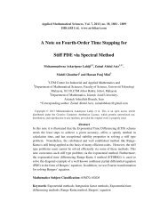
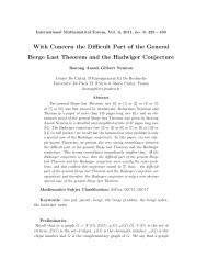
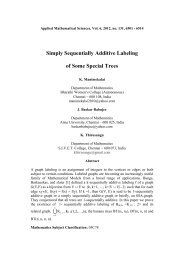
For N=8, j=8, the graph <strong>of</strong> solution <strong>of</strong> exact solution and wavelet solution<br />
2<br />
1<br />
0<br />
-1<br />
D8, 256 points.<br />
Exact solution<br />
WG Solution<br />
-2<br />
0<br />
0.015<br />
0.1 0.2 0.3 0.4 0.5<br />
x<br />
Error.<br />
0.6 0.7 0.8 0.9 1<br />
0.01<br />
0.005<br />
0<br />
0 0.1 0.2 0.3 0.4 0.5<br />
x<br />
0.6 0.7 0.8 0.9 1
<strong>Wavelet</strong> <strong>Galerkin</strong> solutions 421<br />
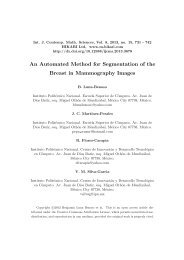
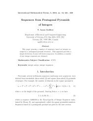
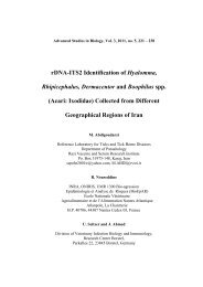
For N=6, j=8, the graph <strong>of</strong> solution <strong>of</strong> exact solution and wavelet solution<br />
2<br />
1<br />
0<br />
-1<br />
D6, 256 points.<br />
-2<br />
0<br />
0.015<br />
0.1 0.2 0.3 0.4 0.5<br />
x<br />
Error.<br />
0.6 0.7 0.8 0.9 1<br />
0.01<br />
0.005<br />
Exact solution<br />
WG solution<br />
0<br />
0 0.1 0.2 0.3 0.4 0.5<br />
x<br />
0.6 0.7 0.8 0.9 1
422 V. Mishra and Sabina<br />
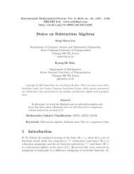
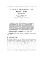
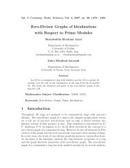
For N=6, j=9, graph shows that error decreases between exact and wavelet solution.<br />
2<br />
1<br />
0<br />
-1<br />
D6, 512 points.<br />
-2<br />
0 0.1 0.2 0.3 0.4 0.5<br />
x<br />
0.6 0.7 0.8 0.9 1<br />
x 10-3<br />
Error.<br />
4<br />
3<br />
2<br />
1<br />
Exact solution<br />
WG solution<br />
0<br />
0 0.1 0.2 0.3 0.4 0.5<br />
x<br />
0.6 0.7 0.8 0.9 1
<strong>Wavelet</strong> <strong>Galerkin</strong> solutions 423<br />
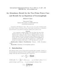
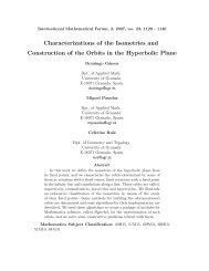
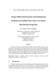
For N=12, j=10, graph shows that error decreases between exact and wavelet<br />
solution.<br />
2<br />
1<br />
0<br />
-1<br />
-2<br />
0 0.1 0.2 0.3 0.4 0.5<br />
x<br />
0.6 0.7 0.8 0.9 1<br />
x 10-4<br />
Error.<br />
8<br />
6<br />
4<br />
2<br />
6. Conclusion<br />
D12, 1024 points.<br />
Exact solution<br />
WG Solution<br />
0<br />
0 0.1 0.2 0.3 0.4 0.5<br />
x<br />
0.6 0.7 0.8 0.9 1<br />
The wavelet method has been shown to be a powerful numerical tool for the fast and<br />
accurate solution <strong>of</strong> differential equations. <strong>Solutions</strong> obtained using the Daubechies<br />
6, 8 and 12 coefficients wavelets have been compared with the exact solutions. In<br />
solving harmonic equation 훼 is chosen to be 891. Matching solutions are obtained<br />
for N=6, j=9 and N=12, j=10. Condition numbers for D12 are constantly lower than<br />
for D6, less errors are shown for former. Dianfeng et al. [11] is silent for higher<br />
values <strong>of</strong> resolution near resonance point but here good solution is shown to exist for<br />
D12.<br />
(<br />
t)<br />
N 1<br />
<br />
n0<br />
h(<br />
n)<br />
2<br />
1/<br />
2<br />
(<br />
2t<br />
n)
424 V. Mishra and Sabina<br />
References<br />
[1] A. Latto, H.L. Resnik<strong>of</strong>f and E. Tenenbaum, The Evaluation <strong>of</strong> Connection<br />
Coefficients <strong>of</strong> Compactly Supported <strong>Wavelet</strong>s, in: Proceedings <strong>of</strong> the French-USA<br />
Workshop on <strong>Wavelet</strong>s and Turbulence, Princeton, New York, 1991, Springer-<br />
Verlag, 1992.<br />
[2] Bjorn Jawerth and Wim Sweldens, <strong>Wavelet</strong>s Multiresolution Analysis Adapted<br />
for Fast Solution <strong>of</strong> Boundary Value <strong>Ordinary</strong> <strong>Differential</strong> <strong>Equations</strong>, Proc. 6 th Cop.<br />
Mount Multi. Conf., April 1993, NASA Conference Pub., 259--273.<br />
[3] G. Belkin, R. Coifman and V. Rokhlin, Fast <strong>Wavelet</strong> Transforms and Numerical<br />
Algorithms, Comm. Pure Appl. Math. 44 (1997), 141-183.<br />
[4] J.-C. Xu and W.-C. Shann, <strong>Wavelet</strong>-<strong>Galerkin</strong> Methods for Two-point Boundary<br />
Value Problems, Num. Math. Eng. 37(1994), 2703-2716.<br />
[5] J. R. Williams and K. Amaratunga, <strong>Wavelet</strong> Based Green’s Function Approach<br />
to 2D PDEs, Engg. Comput.10 (1993), 349-367.<br />
[6] J. R. Williams and K. Amaratunga, High Order wavelet Extrapolation Schemes<br />
for Initial Problems and Boundary Value Problems, July 1994, IESL Tech. Rep., No.<br />
94-07, Intelligent Engineering Systems Laboratory, MIT.<br />
[7] J.R. Williams and Kelvin Amaratunga, Simulation Based Design using <strong>Wavelet</strong>s,<br />
Intelligent Engineering Systems Laboratory, MIT (USA).<br />
[8] Jordi Besora, <strong>Galerkin</strong> <strong>Wavelet</strong> Method for Global Waves in 1D, Master Thesis,<br />
Royal Inst. <strong>of</strong> Tech. Sweden, 2004.<br />
[9] K. Amaratunga, J.R. Williams, S. Qian and J. Weiss, <strong>Wavelet</strong>-<strong>Galerkin</strong> solutions<br />
for one Dimensional Partial <strong>Differential</strong> <strong>Equations</strong>, IESL Technical Report No. 92-<br />
05, Intelligent Engineering Systems Laboratory, M. I. T ., 1992.<br />
[10] K. Amaratunga and J.R. William, <strong>Wavelet</strong>-<strong>Galerkin</strong> <strong>Solutions</strong> for Onedimensional<br />
Partial <strong>Differential</strong> <strong>Equations</strong>, Inter. J. Num. Meth. Eng. 37(1994),<br />
2703-2716.<br />
[11] L.U. Dianfeng, Tadashi Ohyoshi and Lin ZHU, Treatment <strong>of</strong> Boundary<br />
Condition in the Application <strong>of</strong> <strong>Wavelet</strong>–<strong>Galerkin</strong> Method to a SH Wave Problem,<br />
1996, Akita Univ. (Japan).<br />
[12] M.W. Frazier, An Introduction to <strong>Wavelet</strong>s through Linear Algebra, Springer,<br />
New York, 1999.<br />
[13] Stephan Dhalke and Ilona Weinreich, <strong>Wavelet</strong>-<strong>Galerkin</strong> Methods: An Adapted<br />
Biorthogonal <strong>Wavelet</strong> Basis, Constructive Approximation 9 (1993), 237-262.<br />
[14] Ole Christensen, Frames, Riesz Basdes, and Discrete Gabor/<strong>Wavelet</strong><br />
Expansions, Bulletin (New Series) <strong>of</strong> the American Mathematical Society 38 (2001),<br />
273-291.<br />
Received: September, 2010