criticisms of the einstein field equation - Alpha Institute for Advanced ...
criticisms of the einstein field equation - Alpha Institute for Advanced ...
criticisms of the einstein field equation - Alpha Institute for Advanced ...

You also want an ePaper? Increase the reach of your titles
YUMPU automatically turns print PDFs into web optimized ePapers that Google loves.
CRITICISMS OF THE<br />
EINSTEIN FIELD<br />
EQUATION<br />
THE END OF 20TH CENTURY PHYSICS<br />
Myron W. Evans, Stephen J. Cro<strong>the</strong>rs, Horst Eckardt, Kerry Pendergast<br />
March 21, 2010
This book is decicated to<br />
"True Progress <strong>of</strong> Natural Philosophy"<br />
i
Preface<br />
This monograph evolved out <strong>of</strong> Einstein Cartan Evans (ECE) <strong>field</strong> <strong>the</strong>ory when<br />
an investigation was being made <strong>of</strong> <strong>the</strong> inhomogeneous <strong>field</strong> <strong>equation</strong>. This<br />
involved <strong>the</strong> calculation <strong>of</strong> a quantity which in <strong>the</strong> shorthand notation <strong>of</strong> ECE<br />
<strong>the</strong>ory (see www.aias.us) is denoted R ∧ q. Here R is <strong>the</strong> Hodge dual <strong>of</strong> <strong>the</strong><br />
curvature <strong>for</strong>m and q is <strong>the</strong> Cartan tetrad <strong>for</strong>m. The symbol ∧ denotes Cartan’s<br />
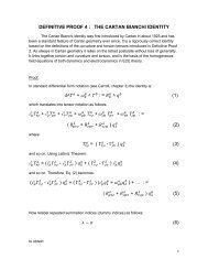
wedge product. The Cartan Evans identity states that:<br />
D ∧ T := R ∧ q (1)<br />
and in <strong>the</strong> Einstein <strong>field</strong> <strong>equation</strong> <strong>the</strong> Hodge dual torsion T is zero. In tensor<br />
notation Eq. (1) becomes:<br />
DµT κµν κ µν<br />
:= R µ<br />
where T κµν κ µν<br />
is <strong>the</strong> torsion tensor in four dimensional spacetime, and where R µ<br />
is <strong>the</strong> curvature tensor. The latter can be worked out from <strong>the</strong> Einstein <strong>field</strong><br />
<strong>equation</strong>, so Eq. (2) gives a new test <strong>for</strong> this <strong>equation</strong>. The curvature tensor<br />
κ µν R µ should be zero because <strong>the</strong> Einstein <strong>field</strong> <strong>equation</strong> uses a zero torsion<br />
T κµν κ µν<br />
by construction. I proceeded to work out R µ by hand, but soon found<br />
that this was far too laborious. Thereafter, in mid 2007, Horst Eckardt and his<br />
κ µν<br />
group in Munich wrote code <strong>for</strong> <strong>the</strong> evaluation <strong>of</strong> R µ by computer algebra.<br />
This resulted in paper 93 on www.aias.us and came up with <strong>the</strong> important<br />
κ µν<br />
finding that <strong>the</strong> Einstein <strong>field</strong> <strong>equation</strong> gives a non zero R µ in general, and<br />
is <strong>the</strong>re<strong>for</strong>e wholly incorrect.<br />
This finding was <strong>the</strong>reafter rein<strong>for</strong>ced by later papers <strong>of</strong> <strong>the</strong> ECE series,<br />
which showed that every known metric <strong>of</strong> <strong>the</strong> Einstein <strong>field</strong> <strong>equation</strong> is incorrect.<br />
In paper 122 <strong>of</strong> <strong>the</strong> ECE series <strong>the</strong> root cause <strong>of</strong> this disaster <strong>for</strong> <strong>the</strong> now obsolete<br />
physics <strong>of</strong> <strong>the</strong> twentieth century was discovered, <strong>the</strong> connection in Riemannian<br />
geometry must be antisymmetric in its lower two indices µ and ν. For some<br />
obscure reason Einstein and his contemporaries used a symmetric connection,<br />
an elementary error. The antisymmetry <strong>of</strong> <strong>the</strong> connection is shown easily as<br />
follows. Define <strong>the</strong> commutator <strong>of</strong> covariant derivatives in any four dimensional<br />
spacetime:<br />
Dµν = −Dνµ := [Dµ, Dν]. (3)<br />
<strong>the</strong>n well known textbook calculations show that:<br />
DµνV ρ = R ρ σµνV σ − T λ µν DλV ρ<br />
iii<br />
(2)<br />
(4)
PREFACE<br />
where R ρ σµν is <strong>the</strong> curvature tensor, T λ µν is <strong>the</strong> torsion tensor, V ρ is a vector<br />
and DλV ρ is its covariant derivative. The torsion tensor is defined by:<br />
T λ µν = Γ λ µν − Γ λ νµ<br />
where Γ λ µν is <strong>the</strong> connection. The latter <strong>the</strong>re<strong>for</strong>e has <strong>the</strong> same symmetry as<br />
<strong>the</strong> commutator, i.e. it is antisymmetric in µ and ν:<br />
Γ λ µν = −Γ λ νµ. (6)<br />
Both <strong>the</strong> commutator and <strong>the</strong> connection vanish if µ is <strong>the</strong> same as ν. This<br />
means that <strong>the</strong> torsion and curvature vanish if µ is <strong>the</strong> same as ν. The error<br />
made by Einstein, and repeated until <strong>the</strong> evolution <strong>of</strong> ECE, was:<br />
Γ λ µν =? Γ λ νµ =? 0. (7)<br />
This error, and its repetition <strong>for</strong> ninety years, is inexplicable in logic, it is<br />
perhaps due to belief retention. When we submitted paper 93 to Physica B<br />
in 2007/2008 it was met by crude personal abuse, so this seems indeed to be<br />
hostility due to belief retention, a commonplace human failing. This means that<br />
academic physics itself comes under <strong>the</strong> microscope, being a clearly unreliable<br />
subject. Schroedinger, and independently, Bauer, were <strong>the</strong> first to criticise <strong>the</strong><br />
Einstein <strong>field</strong> <strong>equation</strong> in 1918, and <strong>the</strong>se <strong>criticisms</strong> have echoed down <strong>the</strong> years.<br />
Academic physics seems to have ignored <strong>the</strong>m illogically.<br />
The use <strong>of</strong> <strong>the</strong> antisymmetric connection led to important new antisymmetry<br />
laws which have been developed in later papers <strong>of</strong> <strong>the</strong> ECE series, papers<br />
which attract a huge readership <strong>of</strong> high quality on www.aias.us, but which are<br />
ana<strong>the</strong>ma to academic physics. The latter has <strong>the</strong>re<strong>for</strong>e been isolated as a<br />
non-scientific remnant by o<strong>the</strong>r scientific pr<strong>of</strong>essions, by industry, government,<br />
military staffs and individual scholars in <strong>the</strong>ir hundreds <strong>of</strong> thousands.<br />
Once it is accepted that <strong>the</strong> connection is antisymmetric in its lower two<br />
indices, its Hodge dual may be defined as in <strong>the</strong> textbooks:<br />
Γ λ µν = 1<br />
2 g1/2 ɛ αβ<br />
µν Γ λ αβ (8)<br />
where g1/2 is <strong>the</strong> square root <strong>of</strong> <strong>the</strong> positive value <strong>of</strong> <strong>the</strong> determinant <strong>of</strong> <strong>the</strong><br />
metric, a weighting factor which cancels out in later calculations. In Eq. (8)<br />
<strong>the</strong> totally antisymmetric unit tensor ɛ αβ<br />
µν is defined as <strong>the</strong> flat space tensor.<br />
The Hodge dual torsion is <strong>the</strong> tensor:<br />
T λ µν = Γ λ µν − Γ λ νµ. (9)<br />
Nei<strong>the</strong>r <strong>the</strong> connection nor <strong>the</strong> Hodge dual connection are tensors, because<br />
under <strong>the</strong> general coordinate trans<strong>for</strong>mation <strong>the</strong>y do not trans<strong>for</strong>m as tensors.<br />
They are never<strong>the</strong>less antisymmetric in <strong>the</strong>ir lower two indices. The Hodge dual<br />
trans<strong>for</strong>mation applied to Eq. (4) produces:<br />
DµνV ρ = R ρ σµνV σ − T λ µν DλV ρ<br />
iv<br />
(5)<br />
(10)
PREFACE<br />
in which <strong>the</strong> structure <strong>of</strong> <strong>the</strong> torsion tensor must be defined as in Eq. (9). It<br />
follows that <strong>the</strong> covariant derivative used in Eq. (10) must be:<br />
DµV ρ = ∂µV ρ + Γ ρ λ<br />
µλV and that <strong>the</strong> Hodge dual curvature tensor must be:<br />
(11)<br />
R ρ σµν = ∂µ Γ ρ νσ − ∂ν Γ ρ µσ + Γ ρ<br />
µλ Γ λ νσ − Γ ρ<br />
νλ Γ λ µσ. (12)<br />
The two tensors (9) and (12) must <strong>the</strong>re<strong>for</strong>e give a new identity <strong>of</strong> differential<br />
geometry:<br />
D ∧ T a := d ∧ T a + ω a b ∧ T b := R a b ∧ q b<br />
(13)<br />
which has become known as <strong>the</strong> Cartan Evans identity. The original Cartan<br />
identity is well known from <strong>the</strong> textbooks to be:<br />
D ∧ T a := d ∧ T a + ω a b ∧ T b := R a b ∧ q b . (14)<br />
The Cartan Evans identity (13) shows that <strong>the</strong> Einstein <strong>field</strong> <strong>equation</strong> is incorrect,<br />
as explained already in this preface, and this book is dedicated to this<br />
demonstration, with chapters by o<strong>the</strong>r colleagues who have independently refuted<br />
<strong>the</strong> Einstein <strong>field</strong> <strong>equation</strong> and standard cosmology with its pseudoscientific<br />
contrivances.<br />
The Cartan Evans identity is Hodge dual invariant with <strong>the</strong> Cartan identity.<br />
The <strong>for</strong>mer identity in tensor notation is:<br />
Dµ T a νρ + Dρ T a µν + Dν T a ρµ := R a µνρ + R a ρµν + R a νρµ<br />
which is <strong>the</strong> same as:<br />
DµT aµν a µν<br />
:= R µ<br />
in which <strong>the</strong> covariant derivative is defined by:<br />
(15)<br />
(16)<br />
DµV ρ := ∂µV ρ + Γ ρ<br />
µλ V λ . (17)<br />
A special case <strong>of</strong> Eq. (16) is:<br />
DµT κµν κ µν<br />
:= R µ . (18)<br />
The Cartan identity in tensor notation is:<br />
DµT a νρ + DρT a µν + DνT a ρµ := R a µνρ + R a ρµν + R a νρµ<br />
which is <strong>the</strong> same as:<br />
Dµ T aµν := a µν<br />
R µ<br />
in which <strong>the</strong> covariant derivative is<br />
(19)<br />
(20)<br />
DµV ρ := ∂µV ρ + Γ ρ<br />
µλ V λ . (21)<br />
A special case <strong>of</strong> Eq. (20) is<br />
Dµ T κµν := κ µν<br />
R µ . (22)<br />
v
PREFACE<br />
Craigcefnparc, Wales Myron W. Evans<br />
October 2009 The British and Commonwealth Civil List Scientist<br />
vi
Contents<br />
1 Introduction 5<br />
2 A Review <strong>of</strong> Einstein Cartan Evans (ECE) Field Theory 9<br />
2.1 Introduction . . . . . . . . . . . . . . . . . . . . . . . . . . . . . . 9<br />
2.2 Geometrical Principles . . . . . . . . . . . . . . . . . . . . . . . . 13<br />
2.3 The Field and Wave Equations <strong>of</strong> ECE Theory . . . . . . . . . . 15<br />
2.4 Aharonov Bohm and Phase Effects in ECE Theory . . . . . . . . 20<br />
2.5 Tensor and Vector Laws <strong>of</strong> Classical Dynamics and Electrodynamics 28<br />
2.6 Spin Connection Resonance . . . . . . . . . . . . . . . . . . . . . 37<br />
2.7 Effects <strong>of</strong> Gravitation on Optics and Spectroscopy . . . . . . . . 41<br />
2.8 Radiative Corrections in ECE Theory . . . . . . . . . . . . . . . 46<br />
2.9 Summary <strong>of</strong> Advances Made by ECE Theory, and Criticisms <strong>of</strong><br />
<strong>the</strong> Standard Model . . . . . . . . . . . . . . . . . . . . . . . . . 53<br />
2.10 Appendix 1: Homogeneous Maxwell Heaviside Equations . . . . . 59<br />
2.11 Appendix 2: The Inhomogeneous Equations . . . . . . . . . . . . 61<br />
2.12 Appendix 3: Some Examples <strong>of</strong> Hodge Duals in Minkowski Space-<br />
Time . . . . . . . . . . . . . . . . . . . . . . . . . . . . . . . . . . 63<br />
2.13 Appendix 4: Standard Tensorial Formulation <strong>of</strong> <strong>the</strong> Homogeneous<br />
Maxwell Heaviside Field Equations . . . . . . . . . . . . . 65<br />
2.14 Appendix 5: Illustrating <strong>the</strong> Meaning <strong>of</strong> <strong>the</strong> Connection with<br />
Rotation in a Plane . . . . . . . . . . . . . . . . . . . . . . . . . . 69<br />
3 Fundamental Errors in <strong>the</strong> General Theory <strong>of</strong> Relativity 85<br />
3.1 Introduction . . . . . . . . . . . . . . . . . . . . . . . . . . . . . . 85<br />
3.2 Schwarzschild spacetime . . . . . . . . . . . . . . . . . . . . . . . 86<br />
3.3 Spherical Symmetry . . . . . . . . . . . . . . . . . . . . . . . . . 88<br />
3.4 Derivation <strong>of</strong> Schwarzschild spacetime . . . . . . . . . . . . . . . 93<br />
3.5 The prohibition <strong>of</strong> point-mass singularities . . . . . . . . . . . . . 102<br />
3.6 Laplace’s alleged black hole . . . . . . . . . . . . . . . . . . . . . 103<br />
3.7 Black hole interactions and gravitational collapse . . . . . . . . . 106<br />
3.8 Fur<strong>the</strong>r consequences <strong>for</strong> gravitational waves . . . . . . . . . . . 109<br />
3.9 O<strong>the</strong>r Violations . . . . . . . . . . . . . . . . . . . . . . . . . . . 117<br />
3.10 Three-dimensional spherically symmetric metric manifolds - first<br />
principles . . . . . . . . . . . . . . . . . . . . . . . . . . . . . . . 122<br />
1
CONTENTS<br />
3.11 Conclusions . . . . . . . . . . . . . . . . . . . . . . . . . . . . . . 125<br />
4 Violation <strong>of</strong> <strong>the</strong> Dual Bianchi Identity by Solutions <strong>of</strong> <strong>the</strong> Einstein<br />
Field Equation 133<br />
4.1 Introduction . . . . . . . . . . . . . . . . . . . . . . . . . . . . . . 133<br />
4.2 Numerical procedure . . . . . . . . . . . . . . . . . . . . . . . . . 135<br />
4.3 Results and discussion . . . . . . . . . . . . . . . . . . . . . . . . 136<br />
4.4 Exact solutions <strong>of</strong> <strong>the</strong> Einstein Field Equation . . . . . . . . . . 141<br />
4.4.1 Minkowski metric with shifted radial coordinate . . . . . 143<br />
4.4.2 Schwarzschild metric . . . . . . . . . . . . . . . . . . . . . 145<br />
4.4.3 General Cro<strong>the</strong>rs metric . . . . . . . . . . . . . . . . . . . 149<br />
4.4.4 Cro<strong>the</strong>rs metric with generalized Schwarzschild parameters 154<br />
4.4.5 Cro<strong>the</strong>rs metric with Schwarzschild parameters . . . . . . 163<br />
4.4.6 General spherical metric . . . . . . . . . . . . . . . . . . . 168<br />
4.4.7 Spherically symmetric metric with perturbation a/r . . . 173<br />
4.4.8 Spherically symmetric metric with general µ(r) . . . . . . 179<br />
4.4.9 Spherically symmetric metric with <strong>of</strong>f-diagonal elements . 184<br />
4.4.10 Reissner-Nordstrom metric . . . . . . . . . . . . . . . . . 191<br />
4.4.11 Extended Reissner-Weyl metric . . . . . . . . . . . . . . . 199<br />
4.4.12 Kerr metric . . . . . . . . . . . . . . . . . . . . . . . . . . 204<br />
4.4.13 Kerr-Newman (Charged Kerr metric) with M = 0, ρ =<br />
const. . . . . . . . . . . . . . . . . . . . . . . . . . . . . . 219<br />
4.4.14 Kerr-Newman (Charged Kerr metric) with a = 0 . . . . . 227<br />
4.4.15 Goedel metric . . . . . . . . . . . . . . . . . . . . . . . . . 231<br />
4.4.16 Static De Sitter metric . . . . . . . . . . . . . . . . . . . . 236<br />
4.4.17 FLRW metric . . . . . . . . . . . . . . . . . . . . . . . . . 244<br />
4.4.18 Closed FLRW metric . . . . . . . . . . . . . . . . . . . . . 249<br />
4.4.19 Friedmann Dust metric . . . . . . . . . . . . . . . . . . . 262<br />
4.4.20 Kasner metric . . . . . . . . . . . . . . . . . . . . . . . . . 268<br />
4.4.21 Generalized FLRW metric . . . . . . . . . . . . . . . . . . 272<br />
4.4.22 Eddington-Finkelstein metric <strong>for</strong> black holes . . . . . . . . 279<br />
4.4.23 Kruskal coordinates metric <strong>of</strong> black hole . . . . . . . . . . 283<br />
4.4.24 Einstein-Rosen bridge metric, u cordinates . . . . . . . . 290<br />
4.4.25 Einstein-Rosen bridge metric, r coordinates . . . . . . . . 294<br />
4.4.26 Massless Einstein-Rosen bridge metric, r coordinates . . . 298<br />
4.4.27 General Morris-Thorne wormhole metric . . . . . . . . . . 304<br />
4.4.28 Bekenstein-Hawking radiation metric . . . . . . . . . . . . 308<br />
4.4.29 Multi-cosmic string metric . . . . . . . . . . . . . . . . . . 313<br />
4.4.30 Multi-cosmic string metric, bicone . . . . . . . . . . . . . 317<br />
4.4.31 Einstein-Rosen type cosmic string metric . . . . . . . . . 320<br />
4.4.32 Wheeler-Misner wormhole by 2 cosmic strings . . . . . . . 323<br />
4.4.33 Hayward-Kim-Lee wormhole type 1 . . . . . . . . . . . . 326<br />
4.4.34 Hayward-Kim-Lee wormhole type 2 . . . . . . . . . . . . 330<br />
4.4.35 Simple Wormhole metric . . . . . . . . . . . . . . . . . . . 335<br />
4.4.36 Simple wormhole metric with varying cosmological constant338<br />
4.4.37 Evans metric . . . . . . . . . . . . . . . . . . . . . . . . . 343<br />
2
CONTENTS<br />
4.4.38 Perfect spherical fluid metric . . . . . . . . . . . . . . . . 349<br />
4.4.39 Carmeli metric <strong>for</strong> spiral galaxies . . . . . . . . . . . . . . 354<br />
4.4.40 Dirac metric . . . . . . . . . . . . . . . . . . . . . . . . . 359<br />
4.4.41 Alcubierre metric . . . . . . . . . . . . . . . . . . . . . . . 367<br />
4.4.42 Homogeneous Space-Time . . . . . . . . . . . . . . . . . . 382<br />
4.4.43 Robertson-Walker metric . . . . . . . . . . . . . . . . . . 388<br />
4.4.44 Anti-Mach metric . . . . . . . . . . . . . . . . . . . . . . 393<br />
4.4.45 Petrov metric . . . . . . . . . . . . . . . . . . . . . . . . . 396<br />
4.4.46 Homogeneous non-null electromagnetic <strong>field</strong>s, type 1 . . . 403<br />
4.4.47 Homogeneous non-null electromagnetic <strong>field</strong>s, type 2 . . . 408<br />
4.4.48 Homogeneous perfect fluid, spherical . . . . . . . . . . . . 417<br />
4.4.49 Homogeneous perfect fluid, cartesian . . . . . . . . . . . . 423<br />
4.4.50 Petrov type N metric . . . . . . . . . . . . . . . . . . . . . 428<br />
4.4.51 Space Rotationally Isotropic Metric . . . . . . . . . . . . 432<br />
4.4.52 Electrovacuum metric . . . . . . . . . . . . . . . . . . . . 440<br />
4.4.53 Spatially homogeneous perfect fluid cosmologies . . . . . . 443<br />
4.4.54 The main cosmological models . . . . . . . . . . . . . . . 448<br />
4.4.55 Petrov type D fluid . . . . . . . . . . . . . . . . . . . . . . 453<br />
4.4.56 Spherically symmetric electromagnetic <strong>field</strong> with Λ = 0 . 457<br />
4.4.57 Plane symmetric vacuum metric . . . . . . . . . . . . . . 464<br />
4.4.58 Sheared dust metric . . . . . . . . . . . . . . . . . . . . . 468<br />
4.4.59 Plane-symmetric perfect fluid metric . . . . . . . . . . . . 472<br />
4.4.60 Spherically symmetric perfect fluid metric (static) . . . . 477<br />
4.4.61 Spherically symmetric perfect fluid metric (dynamic) . . . 482<br />
4.4.62 Collision <strong>of</strong> plane waves . . . . . . . . . . . . . . . . . . . 488<br />
5 Einstein’s Great Contributions to Physics, New Cosmologies<br />
and <strong>the</strong> Alternating Theory <strong>of</strong> <strong>the</strong> Universe, as a Replacement<br />
<strong>for</strong> <strong>the</strong> Flawed Big Bang Theory 497<br />
5.1 Introduction . . . . . . . . . . . . . . . . . . . . . . . . . . . . . . 497<br />
5.2 Einstein’s Early Work and how it has been extended by workers<br />
at AIAS . . . . . . . . . . . . . . . . . . . . . . . . . . . . . . . . 498<br />
5.2.1 Einstein’s Miracle Year and Subsequent Work . . . . . . . 498<br />
5.2.2 The Photoelectric Effect, Quantum Theory and <strong>the</strong> Photon500<br />
5.2.3 The Existence and Motion <strong>of</strong> Atoms . . . . . . . . . . . . 501<br />
5.2.4 Special Relativity . . . . . . . . . . . . . . . . . . . . . . . 504<br />
5.2.5 E = mc 2 . . . . . . . . . . . . . . . . . . . . . . . . . . . . 507<br />
5.3 Einstein and General Relativity . . . . . . . . . . . . . . . . . . . 513<br />
5.4 Testing Relativity, by Observing Light Bending Around <strong>the</strong> Sun 517<br />
5.5 Black Holes, Singularities and Large Masses . . . . . . . . . . . . 521<br />
5.6 New Cosmologies . . . . . . . . . . . . . . . . . . . . . . . . . . . 527<br />
5.7 Dark Matter in Focus . . . . . . . . . . . . . . . . . . . . . . . . 539<br />
3
CONTENTS<br />
4
Chapter 1<br />
Introduction<br />
by<br />
Myron W. Evans 1 ,<br />
<strong>Alpha</strong> <strong>Institute</strong> <strong>for</strong> Advance Study (AIAS)<br />
(www.aias.us, www.atomicprecision.com)<br />
This book is a review <strong>of</strong> recent <strong>criticisms</strong> <strong>of</strong> <strong>the</strong> well known Einstein <strong>field</strong><br />
<strong>equation</strong> <strong>of</strong> 1915, which is still <strong>the</strong> basis <strong>for</strong> ideas such as big bang, black holes<br />
and dark matter, and <strong>of</strong> <strong>the</strong> precision tests <strong>of</strong> general relativity in <strong>the</strong> standard<br />
physics. The book is divided into chapters by contemporary critics <strong>of</strong> <strong>the</strong> <strong>equation</strong>.<br />
Chapter two is a review <strong>of</strong> <strong>the</strong> well known Einstein Cartan Evans (ECE)<br />
variation on relativity <strong>the</strong>ory, which correctly considers <strong>the</strong> role <strong>of</strong> space-time<br />
torsion and reinstates torsion in its central role. This chapter is paper 100 on<br />
<strong>the</strong> www.aias.us site, <strong>the</strong> most read site <strong>of</strong> contemporary physics, and gives a<br />
rigorous pro<strong>of</strong> <strong>of</strong> <strong>the</strong> Bianchi identity <strong>of</strong> Cartan geometry and its dual identity.<br />
It is shown that <strong>the</strong> Einstein <strong>field</strong> <strong>equation</strong> does not obey <strong>the</strong>se fundamental<br />
identities <strong>of</strong> geometry because <strong>of</strong> its neglect <strong>of</strong> torsion. Chapter three is by<br />
Stephen Cro<strong>the</strong>rs, a leading scholar on solutions <strong>of</strong> <strong>the</strong> <strong>equation</strong>. In his chapter<br />
Cro<strong>the</strong>rs give several clear arguments as to <strong>the</strong> fundamental incorrectness <strong>of</strong> big<br />
bang, and exposes glaring errors in <strong>the</strong> ma<strong>the</strong>matics <strong>of</strong> such claims. Similarly,<br />
Cro<strong>the</strong>rs shows with clarity and rigor that claims to <strong>the</strong> existence <strong>of</strong> black holes<br />
and dark matter cannot be ma<strong>the</strong>matically correct, and so have no significance<br />
in physics.<br />
Chapter four is by Horst Eckardt, and uses recently developed computer<br />
algebra to show that all ma<strong>the</strong>matical solutions <strong>of</strong> <strong>the</strong> Einstein <strong>field</strong> <strong>equation</strong><br />
in <strong>the</strong> presence <strong>of</strong> finite energy momentum density violate <strong>the</strong> dual identity<br />
proven in chapter two and in several papers on www.aias.us. For each line<br />
element solution <strong>of</strong> <strong>the</strong> Einstein <strong>field</strong> <strong>equation</strong>, computer algebra is used to give<br />
1 e-mail: emyrone@aol.com<br />
5
all <strong>the</strong> Christ<strong>of</strong>fel symbols and all elements <strong>of</strong> <strong>the</strong> Riemann, Ricci and Einstein<br />
tensors. Each line element is checked <strong>for</strong> metric compatibility, and each line<br />
element is checked to see if it obeys <strong>the</strong> fundamental Ricci cyclic <strong>equation</strong>,<br />
known in <strong>the</strong> standard literature as <strong>the</strong> first Bianchi identity. This appellation<br />
<strong>of</strong> <strong>the</strong> standard physics is a misnomer, because it is nei<strong>the</strong>r a true identity<br />
nor was it given by Bianchi. It was first given by Ricci and Levi-Civita. The<br />
rigorously correct Bianchi identity in geometry was first given by Cartan as is<br />
well known, and as is equally well known, must include <strong>the</strong> torsion ineluctably.<br />
Finally in this chapter by Eckardt, <strong>the</strong> line element solutions are tested against<br />
<strong>the</strong> dual identity proven in chapter two. The results are given in tables and<br />
graphs. They are exceedingly intricate, so <strong>the</strong> computer is used to build up <strong>the</strong><br />
tables without manual transcription error. The results show clearly that <strong>the</strong><br />
Einstein <strong>field</strong> <strong>equation</strong> is incorrect geometrically - meaning that <strong>the</strong> standard<br />
<strong>the</strong>ory <strong>of</strong> relativity must be revised fundamentally to place torsion as a central<br />
feature <strong>of</strong> <strong>the</strong> natural and engineering sciences. This is what ECE <strong>the</strong>ory does.<br />
In <strong>the</strong> fifth chapter, Kerry Pendergast uses his skills as an educator and<br />
writer to put <strong>the</strong>se results in historical and scientific context. In so doing he<br />
uses some <strong>of</strong> <strong>the</strong> material from his "virtual best seller" on www.aias.us, called<br />
"Crystal Spheres" to give a historically accurate description <strong>of</strong> <strong>the</strong> evolution <strong>of</strong><br />
<strong>the</strong> <strong>the</strong>ory <strong>of</strong> relativity.<br />
In <strong>the</strong> remainder <strong>of</strong> this introductory chapter a brief account is given <strong>of</strong><br />
<strong>the</strong> evolution <strong>of</strong> space-time torsion in geometry and ECE <strong>the</strong>ory. The latter is<br />
reviewed in detail in chapter two <strong>of</strong> this book, (paper 100 <strong>of</strong> www.aias.us). The<br />
fundamental idea <strong>of</strong> <strong>the</strong> <strong>the</strong>ory <strong>of</strong> relativity is that physics must be an objective<br />
subject independent <strong>of</strong> anthropomorphic bias.<br />
This philosophy was given <strong>for</strong> example by High Renaissance thinkers such<br />
as Bernardino Telesio and Francis Bacon, but goes back to classical times. Its<br />
most well known manifestation appears in <strong>the</strong> Idol <strong>of</strong> <strong>the</strong> Cave philosophy <strong>of</strong><br />
Bacon. By this he means <strong>the</strong> fantasies <strong>of</strong> <strong>the</strong> human mind, <strong>the</strong> word "idol"<br />
being used in its original classical Greek meaning <strong>of</strong> "dream". Bacon asserts<br />
that <strong>the</strong> workings <strong>of</strong> nature must be manifest through empirical testing <strong>of</strong> human<br />
ideas, in our times "experimental data". Contemporary science is based on this<br />
philosophy combined with <strong>the</strong> earlier philosophy <strong>of</strong> William <strong>of</strong> Ockham, that<br />
<strong>the</strong> simpler <strong>of</strong> two <strong>the</strong>ories is preferred in natural philosophy or physics. The<br />
invisible college <strong>of</strong> Francis Bacon later developed into <strong>the</strong> Royal Society, which<br />
espouses <strong>the</strong> Baconian philosophy.<br />
In Newtonian times <strong>the</strong> idea <strong>of</strong> absolute space and <strong>of</strong> absolute time was predominant,<br />
and <strong>the</strong> whole <strong>of</strong> Newtonian mechanics is based on <strong>the</strong> separation<br />
<strong>of</strong> space and time. The anthropomorphic bias <strong>of</strong> <strong>the</strong> human mind makes this<br />
separation seem entirely natural from everyday experience. Time seems to be<br />
moving in one way, in space we can move <strong>for</strong>wards an backwards, and <strong>the</strong> two<br />
concepts appeared to be described by Newtonian mechanics with <strong>the</strong> later addition<br />
<strong>of</strong> <strong>the</strong> Euler, Laplace and Hamilton <strong>equation</strong>s and so <strong>for</strong>th in classical<br />
dynamics. In <strong>the</strong> nineteenth century <strong>the</strong>se well known concepts <strong>of</strong> dynamics<br />
were challenged by <strong>the</strong> <strong>the</strong>n new classical electrodynamics, notably <strong>the</strong> vector<br />
<strong>equation</strong>s <strong>of</strong> Heaviside. These are <strong>the</strong> well known <strong>equation</strong>s <strong>of</strong> classical electro-<br />
6
CHAPTER 1. INTRODUCTION<br />
dynamics, developed from <strong>the</strong> quaternion <strong>equation</strong>s <strong>of</strong> Maxwell and Faraday’s<br />
concept <strong>of</strong> <strong>field</strong> <strong>of</strong> <strong>for</strong>ce which he named <strong>the</strong> electro-tonic state. The Heaviside<br />
<strong>field</strong> <strong>equation</strong>s are misnamed "<strong>the</strong> Maxwell <strong>equation</strong>s" in <strong>the</strong> standard books<br />
in physics, and importantly, are not Newtonian in nature. They are covariant<br />
under <strong>the</strong> Lorentz trans<strong>for</strong>mation, not <strong>the</strong> Galilean trans<strong>for</strong>mation <strong>of</strong> space<br />
separated from time.<br />
Heaviside developed his <strong>equation</strong>s a few years be<strong>for</strong>e Michelson and Morley<br />
proved <strong>the</strong> absence <strong>of</strong> <strong>the</strong> ae<strong>the</strong>r, causing a crisis <strong>of</strong> thought in natural philosophy<br />
as is well known. The results <strong>of</strong> <strong>the</strong> Michelson Morley experiment were<br />
discussed by Heaviside and Fitzgerald, who can be said to be <strong>the</strong> founders <strong>of</strong> <strong>the</strong><br />
<strong>the</strong>ory <strong>of</strong> relativity. This discussion culminated in <strong>the</strong> proposal by Fitzgerald <strong>of</strong><br />
length contraction to explain <strong>the</strong> results <strong>of</strong> <strong>the</strong> Michelson Morley experiment.<br />
This was a qualitative proposal made to <strong>the</strong> journal "Science" and it took a<br />
fur<strong>the</strong>r eight years or so <strong>for</strong> Lorentz to produce <strong>the</strong> <strong>equation</strong>s <strong>of</strong> <strong>the</strong> Lorentz<br />
trans<strong>for</strong>m, in which space and time both trans<strong>for</strong>m. About this time, 1900,<br />
Poincare, Bianchi, Ricci and Levi-Civita began to develop <strong>the</strong> <strong>the</strong>ory <strong>of</strong> tensors,<br />
a term coined by Hamilton. The Heaviside <strong>equation</strong>s were put into tensor<br />
<strong>for</strong>m, <strong>the</strong> electromagnetic <strong>field</strong> was shown to be part <strong>of</strong> a four by four matrix<br />
so that electricity and magnetism became part <strong>of</strong> <strong>the</strong> same entity. In <strong>the</strong> years<br />
1900 to 1905 several scientists contributed to special relativity, and in 1905 Einstein<br />
proposed <strong>the</strong> constancy <strong>of</strong> <strong>the</strong> speed <strong>of</strong> light as a cornerstone and showed<br />
that <strong>the</strong> <strong>equation</strong>s <strong>of</strong> dynamics are Lorentz covariant in special relativity, as<br />
well as <strong>the</strong> Heaviside <strong>equation</strong>s <strong>of</strong> electro-dynamics. Around <strong>the</strong> same time<br />
Minkowski developed <strong>the</strong> contra-variant covariant notation and <strong>the</strong> concept <strong>of</strong><br />
Minkowski space-time, or flat space-time described by <strong>the</strong> metric diag (-1, 1,<br />
1, 1). There<strong>for</strong>e <strong>the</strong> discussions between Heaviside and Fitzgerald culminated<br />
circa 1906 in <strong>the</strong> <strong>the</strong>ory <strong>of</strong> special relativity as still used today. In this <strong>the</strong>ory a<br />
frame translates with constant velocity with respect to a second, and <strong>the</strong> <strong>equation</strong>s<br />
<strong>of</strong> physics retain <strong>the</strong>ir tensor <strong>for</strong>m under <strong>the</strong> Lorentz trans<strong>for</strong>m. It is now<br />
known that special relativity is <strong>the</strong> most precise <strong>the</strong>ory in physics, having been<br />
rigorously tested in many ways.<br />
The development <strong>of</strong> general relativity, in which a frame moves in any way,<br />
i.e. arbitrarily, with respect to ano<strong>the</strong>r, is due to Einstein from about 1906<br />
onwards. The basic tensorial idea <strong>of</strong> general relativity is that <strong>the</strong> <strong>equation</strong>s<br />
<strong>of</strong> physics retain <strong>the</strong>ir <strong>for</strong>m under any type <strong>of</strong> trans<strong>for</strong>mation, and that this<br />
trans<strong>for</strong>mation is a coordinate trans<strong>for</strong>mation in four dimensions (ct, X, Y, Z).<br />
General relativity is a philosophical departure from special relativity because in<br />
<strong>the</strong> <strong>for</strong>mer subject <strong>the</strong> metric is no longer <strong>the</strong> static diag (-1, 1, 1, 1). Also,<br />
physics is thought <strong>of</strong> in terms <strong>of</strong> a geometry that is not Euclidean. Perhaps this<br />
is <strong>the</strong> greatest achievement <strong>of</strong> Einstein, <strong>the</strong> application <strong>of</strong> Riemann geometry to<br />
physics. The fundamental task <strong>of</strong> development <strong>of</strong> <strong>the</strong> Einstein <strong>field</strong> <strong>equation</strong> is<br />
how to make physics proportional to geometry. This is <strong>the</strong> easiest way to think<br />
<strong>of</strong> general relativity because it is not an intuitive concept, nei<strong>the</strong>r is length contraction<br />
nor time dilation, nor space-time nor <strong>the</strong> Lorentz trans<strong>for</strong>m. The well<br />
known Einstein <strong>field</strong> <strong>equation</strong> <strong>of</strong> 1915 was finally arrived at independently by<br />
Einstein and Hilbert after many discussion with experts in tensor <strong>the</strong>ory and<br />
7
geometry such as Levi-Civita and Grossman. The <strong>field</strong> <strong>equation</strong> states that<br />
a quantity in Riemann geometry is proportional to <strong>the</strong> Noe<strong>the</strong>r Theorem <strong>of</strong><br />
physics, <strong>the</strong> latter being essentially <strong>the</strong> conservation laws <strong>of</strong> physics in tensor<br />
<strong>for</strong>m, or generally covariant <strong>for</strong>m. The quantity in geometry is what <strong>the</strong> standard<br />
physics calls <strong>the</strong> second Bianchi identity. The proportionality constant is<br />
k, <strong>the</strong> Einstein constant. The Einstein <strong>field</strong> <strong>equation</strong> <strong>the</strong>n follows by assuming<br />
that <strong>the</strong> covariant derivative on both sides can be removed, so that <strong>the</strong> Einstein<br />
tensor itself is proportional through k to a quantity known as <strong>the</strong> canonical<br />
energy momentum density <strong>of</strong> matter.<br />
This is <strong>the</strong> <strong>equation</strong> that is still used in <strong>the</strong> standard physics to predict such<br />
things as big bang, black holes and dark matter. They are all consequences<br />
<strong>of</strong> <strong>the</strong> Einstein <strong>field</strong> <strong>equation</strong>, which has become dogmatic in nature. As early<br />
as 1918 Bauer and Schroedinger independently showed major shortcomings <strong>of</strong><br />
<strong>the</strong> Einstein <strong>field</strong> <strong>equation</strong> and <strong>the</strong> Eddington experiment is known now to be<br />
essentially an exercise in anthropomorphic bias, lacking entirely <strong>the</strong> precision to<br />
prove <strong>the</strong> <strong>field</strong> <strong>equation</strong> as is so <strong>of</strong>ten claimed in <strong>the</strong> standard physics. In <strong>the</strong><br />
early twenties, Cartan showed that <strong>the</strong> Riemann geometry itself is incomplete<br />
because <strong>of</strong> its lack <strong>of</strong> space-time torsion. The torsion was un<strong>for</strong>tunately eliminated<br />
by Ricci and Levi-Civita through <strong>the</strong>ir use <strong>of</strong> <strong>the</strong> symmetric connection,<br />
<strong>of</strong>ten attributed to Christ<strong>of</strong>fel.<br />
The Einstein <strong>field</strong> <strong>equation</strong> is <strong>the</strong>re<strong>for</strong>e based on a geometry in which torsion<br />
is eliminated arbitrarily. There is no logical justification <strong>for</strong> this elimination <strong>of</strong><br />
torsion. In this book, it is shown what happens when <strong>the</strong> torsion is neglected -<br />
essentially a disaster <strong>for</strong> twentieth century standard physics. The only way in<br />
which standard physics can justify its claims is to assert without logic that torsion<br />
is a ma<strong>the</strong>matical abstraction. In logic, torsion is no more <strong>of</strong> an abstraction<br />
than curvature, on which <strong>the</strong> whole <strong>of</strong> <strong>the</strong> illogical paraphenalia <strong>of</strong> big bang,<br />
black holes and dark matter is based. Chapter two shows essentially how <strong>the</strong><br />
torsion is central to a generally covariant unified <strong>field</strong> <strong>the</strong>ory, <strong>the</strong> ECE <strong>the</strong>ory.<br />
Chapter three by Cro<strong>the</strong>rs show shows <strong>the</strong> vacuum solutions <strong>of</strong> <strong>the</strong> Einstein<br />
<strong>field</strong> <strong>equation</strong> are meaningless, and reveals <strong>the</strong> basic errors repeated down <strong>the</strong><br />
twentieth century by <strong>the</strong> standard physics. Chapter four by Eckardt uses newly<br />
developed computer algebra to show precisely how <strong>the</strong> lack <strong>of</strong> torsion leads to a<br />
basic contradiction with <strong>the</strong> Bianchi identity <strong>of</strong> Cartan in its Hodge dual <strong>for</strong>m,<br />
and chapter five by Pendergast summarizes <strong>the</strong> historical context.<br />
8
Chapter 2<br />
A Review <strong>of</strong> Einstein Cartan<br />
Evans (ECE) Field Theory<br />
by<br />
Myron W. Evans 1 ,<br />
<strong>Alpha</strong> <strong>Institute</strong> <strong>for</strong> Advance Study (AIAS)<br />
(www.aias.us, www.atomicprecision.com)<br />
2.1 Introduction<br />
The well accepted Einstein Cartan Evans (ECE) <strong>field</strong> <strong>the</strong>ory [1,12] is reviewed in<br />
major <strong>the</strong>mes <strong>of</strong> development from Spring 2003 to present in approximately 103<br />
papers and volumes summarized on www.aias.us and www.atomicprecision.com.<br />
Recently a third website, www.telesio-galilei.com, has been associated with <strong>the</strong>se<br />
two main websites <strong>of</strong> <strong>the</strong> <strong>the</strong>ory. Additionally, <strong>the</strong>se websites contain educational<br />
articles by members <strong>of</strong> <strong>the</strong> <strong>Alpha</strong> <strong>Institute</strong> <strong>for</strong> <strong>Advanced</strong> Study (AIAS)<br />
and <strong>the</strong> Telesio-Galilei Association, and also contain an Omnia Opera listing<br />
most <strong>of</strong> <strong>the</strong> collected works <strong>of</strong> <strong>the</strong> present author, including precursor <strong>the</strong>ories<br />
to ECE <strong>the</strong>ory from 1992 to present. Most original papers are available by hyperlink<br />
<strong>for</strong> scholarly study. It is seen in detail from <strong>the</strong> feedback activity sites<br />
<strong>of</strong> <strong>the</strong> three main sites that ECE <strong>the</strong>ory is fully accepted. All <strong>the</strong> 103 papers to<br />
date are read by someone, somewhere every month, and detailed summaries <strong>of</strong><br />
<strong>the</strong> feedback are available on www.aias.us. Additionally ECE <strong>the</strong>ory has been<br />
published in <strong>the</strong> traditional manner: in four journals with anonymous reviewers,<br />
(three <strong>of</strong> <strong>the</strong>m standard model journals), and is constantly internally refereed<br />
by AIAS staff. The latter are like minded pr<strong>of</strong>essionals who have worked vol-<br />
1 e-mail: emyrone@aol.com<br />
9
2.1. INTRODUCTION<br />
untarily on ECE <strong>the</strong>ory and in <strong>the</strong> development <strong>of</strong> AIAS. Computer algebra<br />
(Maxima program) has been developed to check hand calculations <strong>of</strong> ECE <strong>the</strong>ory<br />
and to per<strong>for</strong>m calculations that are too complicated to carry out by hand.<br />
There<strong>for</strong>e a review <strong>of</strong> <strong>the</strong> main <strong>the</strong>mes <strong>of</strong> development and main discoveries <strong>of</strong><br />
ECE <strong>the</strong>ory is timely.<br />
The ECE <strong>the</strong>ory is a suggestion <strong>for</strong> <strong>the</strong> development <strong>of</strong> a generally covariant<br />
unified <strong>field</strong> <strong>the</strong>ory based on <strong>the</strong> principles <strong>of</strong> general relativity, essentially that<br />
natural philosophy is geometry. This principle has been proposed since ancient<br />
times in many ways, but its most well known manifestation is probably <strong>the</strong><br />
work <strong>of</strong> Albert Einstein from about 1906 to 1915, culminating in <strong>the</strong> proposal<br />
<strong>of</strong> <strong>the</strong> well known Einstein Hilbert (EH) <strong>field</strong> <strong>equation</strong> <strong>of</strong> gravitation. This<br />
work by Einstein and contemporaries is very well known, but a brief summary<br />
is given here. After several false starts Einstein proposed in 1915 that <strong>the</strong><br />
so called “second Bianchi identity” <strong>of</strong> Riemann geometry be proportional to<br />
a <strong>for</strong>m <strong>of</strong> <strong>the</strong> Noe<strong>the</strong>r Theorem in which <strong>the</strong> covariant derivative vanishes <strong>of</strong><br />
<strong>the</strong> canonical energy-momentum tensor. It is much less well known that in so<br />
doing, Einstein used <strong>the</strong> only type <strong>of</strong> geometry <strong>the</strong>n available to him: Riemann<br />
geometry without torsion. The EH <strong>field</strong> <strong>equation</strong> follows from this proposal by<br />
Einstein as a special case:<br />
Gµν = kTµν<br />
(2.1)<br />
where Gµν is <strong>the</strong> Einstein tensor, k is <strong>the</strong> Einstein constant, and Tµν is <strong>the</strong><br />
canonical energy - momentum tensor. Eq. (2.1) is a special case <strong>of</strong> <strong>the</strong> Einstein<br />
proposal <strong>of</strong> 1915:<br />
D µ Gµν = kD µ Tµν = 0 (2.2)<br />
where on <strong>the</strong> left hand side appears geometry, and on <strong>the</strong> right hand side appears<br />
natural philosophy. David Hilbert proposed <strong>the</strong> same <strong>equation</strong> at about<br />
<strong>the</strong> same time using Lagrangian principles, but Hilbert’s work was motivated by<br />
Einstein’s ideas, so <strong>the</strong> EH <strong>equation</strong> is usually attributed to Einstein. The EH<br />
<strong>equation</strong> applies however only to gravitation, whereas ECE has unified general<br />
relativity with <strong>the</strong> o<strong>the</strong>r <strong>field</strong>s <strong>of</strong> nature besides gravitation. The o<strong>the</strong>r fundamental<br />
<strong>field</strong>s are thought to be <strong>the</strong> electromagnetic, weak and strong <strong>field</strong>s.<br />
ECE has also unified general relativity with quantum mechanics by discarding<br />
<strong>the</strong> acausality and subjectivity <strong>of</strong> <strong>the</strong> Copenhagen School, and by deriving objective<br />
and causal wave <strong>equation</strong>s from geometrical first principles. The two<br />
major and well accepted achievements <strong>of</strong> ECE <strong>the</strong>ory are <strong>the</strong>re<strong>for</strong>e <strong>the</strong> unification<br />
<strong>of</strong> <strong>field</strong>s using geometry, and <strong>the</strong> unification <strong>of</strong> relativity and quantum<br />
mechanics. This review is organized in sections outlining <strong>the</strong> main <strong>the</strong>mes and<br />
discoveries <strong>of</strong> ECE <strong>the</strong>ory, and into detailed technical appendices dealing with<br />
basics. These appendices include flow charts <strong>of</strong> <strong>the</strong> inter-relation <strong>of</strong> <strong>the</strong> main<br />
<strong>equation</strong>s.<br />
In Section 2.2 <strong>the</strong> geometrical first principles <strong>of</strong> ECE <strong>the</strong>ory are summarized<br />
briefly, <strong>the</strong> <strong>the</strong>ory is based on a <strong>for</strong>m <strong>of</strong> geometry developed [13] by Cartan<br />
and first published in 1922. This geometry is fully self-consistent and well<br />
10
CHAPTER 2. A REVIEW OF EINSTEIN CARTAN EVANS (ECE) . . .<br />
known - it can be regarded as <strong>the</strong> standard differential geometry taught in good<br />
universities. The dialogue between Einstein and Cartan on this geometry is<br />
perhaps not as well known as <strong>the</strong> dialogue between Einstein and Bohr, but is <strong>the</strong><br />
basis <strong>for</strong> <strong>the</strong> development <strong>of</strong> ECE <strong>the</strong>ory. It is named “Einstein Cartan Evans”<br />
<strong>field</strong> <strong>the</strong>ory because <strong>the</strong> present author set out to suggest a completion <strong>of</strong> <strong>the</strong><br />
Einstein Cartan dialogue. This dialogue was part <strong>of</strong> <strong>the</strong> attempt by Einstein and<br />
many o<strong>the</strong>rs to complete general relativity by developing a generally covariant<br />
unified <strong>field</strong> <strong>the</strong>ory on <strong>the</strong> principles <strong>of</strong> a given geometry. For many reasons<br />
this unification did not come about until Spring <strong>of</strong> 2003, when ECE <strong>the</strong>ory was<br />
proposed. The main obstacles to unification were adherence in <strong>the</strong> standard<br />
model to a U(1) sector <strong>for</strong> electromagnetism, <strong>the</strong> neglect <strong>of</strong> <strong>the</strong> ECE spin <strong>field</strong><br />
B(3), inferred in 1992, and adherence to <strong>the</strong> philosophy <strong>of</strong> <strong>the</strong> Copenhagen<br />
School. Standard model proponents adhere to <strong>the</strong>se principles at <strong>the</strong> time <strong>of</strong><br />
writing, but ECE proponents now adopt a different natural philosophy, since<br />
it may be claimed objectively from feedback data that ECE is a new school <strong>of</strong><br />
thought.<br />
In Section 2.3 <strong>the</strong> main <strong>field</strong> and wave <strong>equation</strong>s <strong>of</strong> ECE are discussed in<br />
summary. They are derived from <strong>the</strong> well known principles <strong>of</strong> Cartan’s geometry.<br />
The gravitational, electromagnetic, weak and strong <strong>field</strong>s are unified by<br />
Cartan’s geometry, each is an aspect <strong>of</strong> <strong>the</strong> same geometry. The <strong>field</strong> <strong>equation</strong>s<br />
are based on <strong>the</strong> one true Bianchi identity given by Cartan, using different representation<br />
spaces. The wave <strong>equation</strong>s are derived from <strong>the</strong> tetrad postulate,<br />
<strong>the</strong> very fundamental requirement in natural philosophy and relativity <strong>the</strong>ory<br />
that <strong>the</strong> complete vector <strong>field</strong> be invariant under <strong>the</strong> general trans<strong>for</strong>mation<br />
<strong>of</strong> coordinates. To translate Cartan to Riemann geometry requires use <strong>of</strong> <strong>the</strong><br />
tetrad postulate. There<strong>for</strong>e both <strong>the</strong> Bianchi identity and tetrad postulate are<br />
fundamentals <strong>of</strong> standard differential geometry and <strong>the</strong>ir use in ECE <strong>the</strong>ory is<br />
entirely standard ma<strong>the</strong>matics [13].<br />
In Section 2.4 <strong>the</strong> unification <strong>of</strong> phase <strong>the</strong>ory made possible by ECE is summarized<br />
in terms <strong>of</strong> <strong>the</strong> main discoveries and points <strong>of</strong> development. The main<br />
point <strong>of</strong> development in this context is <strong>the</strong> unification <strong>of</strong> apparently disparate<br />
phases such as <strong>the</strong> electromagnetic phase, <strong>the</strong> Dirac and Wu Yang phases, and<br />
<strong>the</strong> topological phases. ECE <strong>the</strong>ory presents a unified geometrical approach to<br />
each phase, and this approach also gives a straight<strong>for</strong>ward geometrical explanation<br />
<strong>of</strong> <strong>the</strong> Aharonov Bohm effects and “non-locality”. The electromagnetic<br />
phase <strong>for</strong> example is developed in terms <strong>of</strong> <strong>the</strong> B(3) spin <strong>field</strong> [14] and some<br />
glaring shortcomings <strong>of</strong> <strong>the</strong> standard model are corrected. Thus, apparently<br />
simple and well known effects such as reflection are developed self-consistently<br />
with ECE, while in <strong>the</strong> standard model <strong>the</strong>y are at odds with fundamental symmetry<br />
[1, 12]. The standard model development <strong>of</strong> <strong>the</strong> Aharonov Bohm effects<br />
is also incorrect ma<strong>the</strong>matically, obscure, controversial and convoluted, while in<br />
ECE <strong>the</strong>ory it is straight<strong>for</strong>ward.<br />
In Section 2.5 <strong>the</strong> ECE laws <strong>of</strong> classical dynamics and electrodynamics are<br />
summarized in <strong>the</strong> language <strong>of</strong> vectors, <strong>the</strong> language used in electrical engineering.<br />
The <strong>equation</strong>s <strong>of</strong> electrodynamics in ECE <strong>the</strong>ory reduce to <strong>the</strong> four<br />
laws: Gauss law <strong>of</strong> magnetism, Faraday law <strong>of</strong> induction, Coulomb law and<br />
11
2.1. INTRODUCTION<br />
Ampère Maxwell law. In ECE <strong>the</strong>ory <strong>the</strong>y are <strong>the</strong> same in vector notation as in<br />
<strong>the</strong> familiar Maxwell Heaviside (MH) <strong>field</strong> <strong>the</strong>ory, but in ECE are written in a<br />
different space-time. In ECE <strong>the</strong> electromagnetic <strong>field</strong> is <strong>the</strong> spinning <strong>of</strong> spacetime,<br />
represented by <strong>the</strong> Cartan torsion, while in MH <strong>the</strong> <strong>field</strong> is a nineteenth<br />
century concept still used uncritically in <strong>the</strong> contemporary standard model <strong>of</strong><br />
natural philosophy. The space-time <strong>of</strong> MH is <strong>the</strong> flat and static Minkowski<br />
space-time, while in ECE <strong>the</strong> space-time is dynamic with non-zero curvature<br />
and torsion. This difference manifests itself in <strong>the</strong> relation between <strong>the</strong> <strong>field</strong>s<br />
and potentials in ECE, a relation which includes <strong>the</strong> spin connection.<br />
In Section 2.6, spin connection resonance (SCR) is discussed, concentrating<br />
as usual on <strong>the</strong> main discoveries and points <strong>of</strong> development <strong>of</strong> <strong>the</strong> ECE<br />
<strong>the</strong>ory. In <strong>the</strong>ory, SCR is <strong>of</strong> great practical utility because <strong>the</strong> <strong>equation</strong>s <strong>of</strong><br />
classical electrodynamics become resonance <strong>equation</strong>s <strong>of</strong> <strong>the</strong> type first inferred<br />
by <strong>the</strong> Bernoulli’s and Euler. There<strong>for</strong>e a new source <strong>of</strong> electric power has been<br />
discovered in ECE <strong>the</strong>ory - this source is <strong>the</strong> Cartan torsion <strong>of</strong> space-time. Amplification<br />
occurs in principle through SCR, <strong>the</strong> spin connection itself being <strong>the</strong><br />
property <strong>of</strong> <strong>the</strong> four-dimensional space-time with curvature and torsion which<br />
is <strong>the</strong> base manifold <strong>of</strong> ECE <strong>the</strong>ory. It is well known [15] that <strong>the</strong>se resonance<br />
<strong>equation</strong>s are equivalent to circuits that can be used to amplify electric power.<br />
In all probability <strong>the</strong>se circuits were <strong>the</strong> ones designed by Tesla empirically.<br />
In Section 2.7 <strong>the</strong> utility <strong>of</strong> ECE as a unified <strong>field</strong> <strong>the</strong>ory is illustrated through<br />
<strong>the</strong> effects <strong>of</strong> gravitation in optics and spectroscopy. These are exemplified by<br />
<strong>the</strong> effect <strong>of</strong> gravitation on <strong>the</strong> ring laser gyro (Sagnac effect) and on radiatively<br />
induced fermion resonance (RFR). RFR itself is <strong>of</strong> great potential utility because<br />
it is a <strong>for</strong>m <strong>of</strong> electron and proton spin resonance induced not by a permanent<br />
magnet, but by a circularly polarized electromagnetic <strong>field</strong>. This is known as<br />
<strong>the</strong> inverse Faraday effect (IFE) [16] from which <strong>the</strong> ECE spin <strong>field</strong> B(3) was<br />
inferred in 1992 [17]. The spin <strong>field</strong> signals <strong>the</strong> fact that in a self consistent<br />
philosophy, classical electrodynamics must be part <strong>of</strong> a generally covariant <strong>field</strong><br />
<strong>the</strong>ory. This is incompatible with <strong>the</strong> U(1) sector <strong>of</strong> special relativity still used<br />
to describe electrodynamics in <strong>the</strong> standard model. Any proposal <strong>for</strong> a unified<br />
<strong>field</strong> <strong>the</strong>ory based on U(1) cannot be generally covariant in all sectors, leaving<br />
ECE as <strong>the</strong> only satisfactory unified <strong>field</strong> <strong>the</strong>ory at <strong>the</strong> time <strong>of</strong> writing.<br />
In Section 2.8 <strong>the</strong> well known radiative corrections [18] are developed with<br />
ECE <strong>the</strong>ory, and a summary <strong>of</strong> <strong>the</strong> main points <strong>of</strong> progress illustrated with <strong>the</strong><br />
anomalous g factor <strong>of</strong> <strong>the</strong> electron and <strong>the</strong> Lamb shift. It is shown that claims<br />
to accuracy <strong>of</strong> standard model quantum electrodynamics (QED) are greatly exaggerated.<br />
The accuracy is limited by that <strong>of</strong> <strong>the</strong> Planck constant, <strong>the</strong> least<br />
accurately known fundamental constant appearing in <strong>the</strong> fine structure constant.<br />
There are glaring internal inconsistencies in standards laboratories tables<br />
<strong>of</strong> data on <strong>the</strong> fundamental constants, and QED is based on a number <strong>of</strong> what<br />
are effectively adjustable parameters introduced by ad hoc procedures such as<br />
dimensional renormalization The concepts used in QED are vastly complicated<br />
and are not used in <strong>the</strong> ECE <strong>the</strong>ory <strong>of</strong> <strong>the</strong> experimentally known radiative corrections.<br />
The Feynman perturbation method is not used in ECE: it cannot be<br />
proven to converge as is well known, i.e. needs many terms <strong>of</strong> increasing com-<br />
12
CHAPTER 2. A REVIEW OF EINSTEIN CARTAN EVANS (ECE) . . .<br />
plexity which must be evaluated by computer. So ECE is a fundamental <strong>the</strong>ory<br />
<strong>of</strong> quantized electrodynamics from <strong>the</strong> first principles <strong>of</strong> general relativity, while<br />
QED is a <strong>the</strong>ory <strong>of</strong> special relativity needing adjustable parameters, acausal and<br />
subjective concepts, and <strong>the</strong>re<strong>for</strong>e <strong>of</strong> dubious validity.<br />
In Section 2.9, finally, it is shown that EH <strong>the</strong>ory has several fundamental<br />
shortcomings. As described on ww.telesio-galilei.com EH has been quite severely<br />
criticized down <strong>the</strong> years by several leading physicists. Notably, Cro<strong>the</strong>rs [19]<br />
has criticized <strong>the</strong> methods <strong>of</strong> solution <strong>of</strong> EH, and has shown that uncritically<br />
accepted concepts are in fact incompatible with general relativity. These<br />
include Big Bang, dark hole and dark matter <strong>the</strong>ory and <strong>the</strong> concept <strong>of</strong> a<br />
Ricci flat space-time. He has also shown that <strong>the</strong> use <strong>of</strong> <strong>the</strong> familiar but misnamed<br />
“Schwarzschild metric” is due to lack <strong>of</strong> scholarship and understanding<br />
<strong>of</strong> Schwarzschild’s original papers <strong>of</strong> 1916. ECE has revealed that <strong>the</strong> use <strong>of</strong> <strong>the</strong><br />
familiar Christ<strong>of</strong>fel symbol is incompatible with <strong>the</strong> one true Bianchi identity <strong>of</strong><br />
Cartan. This section suggests a development <strong>of</strong> <strong>the</strong> EH <strong>equation</strong> into one which<br />
is self consistent.<br />
Several technical appendices give basic details which are not usually given<br />
in standard textbooks, but which are never<strong>the</strong>less important to <strong>the</strong> student.<br />
These appendices also contain flow charts inter-relating <strong>the</strong> main concepts and<br />
<strong>equation</strong>s <strong>of</strong> ECE.<br />
2.2 Geometrical Principles<br />
The ECE <strong>the</strong>ory is based on <strong>the</strong> two structure <strong>equation</strong>s <strong>of</strong> Cartan, and <strong>the</strong><br />
Bianchi identity <strong>of</strong> Cartan geometry. During <strong>the</strong> course <strong>of</strong> development <strong>of</strong> <strong>the</strong><br />
<strong>the</strong>ory a useful short-hand notation has been used in which <strong>the</strong> indices are<br />
removed in order to reveal <strong>the</strong> basic structure <strong>of</strong> <strong>the</strong> <strong>equation</strong>s. In this notation<br />
<strong>the</strong> two Cartan structure <strong>equation</strong>s are:<br />
and<br />
T = D ∧ q = d ∧ q + ω ∧ q (2.3)<br />
R = D ∧ ω = d ∧ ω + ω ∧ ω (2.4)<br />
and <strong>the</strong> Bianchi identity is:<br />
D ∧ T = d ∧ T + ω ∧ T := R ∧ q. (2.5)<br />
In this notation T is <strong>the</strong> Cartan torsion <strong>for</strong>m, ω is <strong>the</strong> spin connection symbol,<br />
q is <strong>the</strong> Cartan tetrad <strong>for</strong>m, and R is <strong>the</strong> Cartan curvature <strong>for</strong>m. The meaning<br />
<strong>of</strong> this symbolism is defined in all detail in <strong>the</strong> ECE literature [1, 12], and <strong>the</strong><br />
differential <strong>for</strong>m is defined in <strong>the</strong> standard literature [13]. The purpose <strong>of</strong> this<br />
section is to summarize <strong>the</strong> main advances in basic geometry made during <strong>the</strong><br />
development <strong>of</strong> ECE <strong>the</strong>ory.<br />
The Bianchi identity (2.5) is basic to <strong>the</strong> <strong>field</strong> <strong>equation</strong>s <strong>of</strong> ECE, and its<br />
structure has been developed considerably [1, 12]. It has been shown to be<br />
13
2.2. GEOMETRICAL PRINCIPLES<br />
equivalent to <strong>the</strong> tensor <strong>equation</strong>:<br />
R λ ρµν + R λ µνρ + R λ νρµ<br />
:= ∂νΓ λ ρµ − ∂ρΓ λ νµ + Γ λ νσΓ σ ρµ − Γ λ ρσΓ σ νµ<br />
+ ∂ρΓ λ µν − ∂µΓ λ ρν + Γ λ ρσΓ σ µν − Γ λ µσΓ σ ρν<br />
+ ∂µΓ λ νρ − ∂νΓ λ µρ + Γ λ µσΓ σ νρ − Γ λ νσΓ σ µρ<br />
(2.6)<br />
in which a cyclic sum <strong>of</strong> three Riemann tensors is identically equal to <strong>the</strong> sum <strong>of</strong><br />
three fundamental definitions <strong>of</strong> <strong>the</strong> same Riemann tensors. These fundamental<br />
definitions originate in <strong>the</strong> commutator <strong>of</strong> covariant derivatives acting on a<br />
four-vector in <strong>the</strong> base manifold. The latter is four dimensional space-time with<br />
BOTH curvature and torsion [1, 13]. This operation produces:<br />
[Dµ, Dν]V ρ = R ρ σµνV σ − T λ µνDλV ρ<br />
where <strong>the</strong> torsion tensor is:<br />
(2.7)<br />
T λ µν = Γ λ µν − Γ λ νµ. (2.8)<br />
The curvature or Riemann tensor cannot exist without <strong>the</strong> torsion tensor, and<br />
<strong>the</strong> definition (2.7) has been shown to be equivalent to <strong>the</strong> Bianchi identity<br />
(2.6).<br />
The second advance in basic geometry is <strong>the</strong> inference [1, 12] <strong>of</strong> <strong>the</strong> Hodge<br />
dual <strong>of</strong> <strong>the</strong> Bianchi identity. In short-hand notation this is:<br />
D ∧ T := R ∧ q (2.9)<br />
and is equivalent to:<br />
[Dµ, Dν]HDV ρ = R ρ σµνV σ − T λ µνDλV ρ<br />
(2.10)<br />
where <strong>the</strong> subscript HD denotes Hodge dual. From <strong>the</strong>se considerations it may<br />
be inferred that <strong>the</strong> Bianchi identity and its Hodge dual are <strong>the</strong> tensor <strong>equation</strong>s:<br />
and<br />
Dµ T κµν = R κ µ µν<br />
DµT κµν = R κ µ µν<br />
(2.11)<br />
(2.12)<br />
in which <strong>the</strong> connection is NOT <strong>the</strong> Christ<strong>of</strong>fel connection. Computer algebra<br />
κ µν<br />
[1, 12] has shown that <strong>the</strong> tensor R µ is not zero in general <strong>for</strong> line elements<br />
that use <strong>the</strong> Chrst<strong>of</strong>fel symbol, while T κµν is always zero <strong>for</strong> <strong>the</strong> Christ<strong>of</strong>fel<br />
symbol. So <strong>the</strong> use <strong>of</strong> <strong>the</strong> latter is inconsistent with <strong>the</strong> tensor <strong>equation</strong> (2.12).<br />
There<strong>for</strong>e <strong>the</strong> neglect <strong>of</strong> torsion makes EH <strong>the</strong>ory internally inconsistent, so<br />
standard model general relativity and cosmology are also internally inconsistent<br />
at a basic level. In short-hand notation <strong>the</strong> geometry used in EH is:<br />
R ∧ q = 0 (2.13)<br />
14
CHAPTER 2. A REVIEW OF EINSTEIN CARTAN EVANS (ECE) . . .<br />
which in tensor notation is known as “<strong>the</strong> first Bianchi identity”:<br />
R κ µνρ + R κ ρµν + R κ νρµ = 0 (2.14)<br />
in <strong>the</strong> standard model literature. However, this is not an identity, because it<br />
conflicts with <strong>equation</strong> (2.5), and is true if and only if <strong>the</strong> Christ<strong>of</strong>fel symbol<br />
and symmetric metric are used [1,13]. Eq. (2.14) was actually inferred by Ricci<br />
and Levi-Civita, not by Bianchi. So it is referred to in <strong>the</strong> ECE literature as<br />
<strong>the</strong> Ricci cyclic <strong>equation</strong>.<br />
In <strong>the</strong> course <strong>of</strong> development <strong>of</strong> ECE <strong>the</strong>ory a similar problem was found<br />
with what is referred to in <strong>the</strong> standard model literature as “<strong>the</strong> second Bianchi<br />
identity”. In shorthand notation this is given [13] as:<br />
D ∧ R = 0 (2.15)<br />
but again this neglects torsion. In tensor notation Eq. (2.15) is:<br />
DρR κ σµρ + DµR κ σνρ + DνR κ σρµ = 0. (2.16)<br />
It has been shown [1, 12] that Eq. (2.15) should be:<br />
D ∧ (D ∧ T ) := D ∧ (R ∧ q) (2.17)<br />
which is found by taking D∧ on both sides <strong>of</strong> Eq. (2.15). Eq. (2.17) has been<br />
given in tensor notation [1, 12], and reduces to Eq. (2.16) when:<br />
T λ µν = 0. (2.18)<br />
However, Eq. (2.18) is inconsistent with <strong>the</strong> fundamental operation <strong>of</strong> <strong>the</strong><br />
commutator <strong>of</strong> covariant derivatives on <strong>the</strong> four vector, Eq. (2.7). So in <strong>the</strong> ECE<br />
literature <strong>the</strong> torsion is always considered self-consistently. From <strong>the</strong> fundamentals<br />
[13] <strong>of</strong> Eq. (2.7) <strong>the</strong>re is no a priori reason <strong>for</strong> neglecting torsion, and in<br />
fact <strong>the</strong> torsion tensor is always non-zero if <strong>the</strong> curvature tensor is non-zero.<br />
This fact precludes <strong>the</strong> use <strong>of</strong> <strong>the</strong> Christ<strong>of</strong>fel symbol, making EH <strong>the</strong>ory selfinconsistent.<br />
These are <strong>the</strong> main geometrical advances made during <strong>the</strong> course <strong>of</strong> <strong>the</strong><br />
development <strong>of</strong> ECE <strong>the</strong>ory, which is <strong>the</strong> only self-consistent <strong>the</strong>ory <strong>of</strong> general<br />
relativity. It has also been pointed out by Cro<strong>the</strong>rs [19] that methods <strong>of</strong> solution<br />
<strong>of</strong> <strong>the</strong> EH <strong>equation</strong> are geometrically incorrect, and must be discarded. It<br />
is thought that <strong>the</strong>se errors have been repeated uncritically <strong>for</strong> ninety years<br />
because few have <strong>the</strong> necessary technical ability to understand <strong>the</strong> geometry<br />
<strong>of</strong> general relativity in sufficient depth, and that <strong>the</strong> prestige <strong>of</strong> Einstein has<br />
precluded or inhibited due criticism.<br />
2.3 The Field and Wave Equations <strong>of</strong> ECE Theory<br />
The wave <strong>equation</strong> <strong>of</strong> ECE was <strong>the</strong> first to be developed historically [1,12], and<br />
methods <strong>of</strong> derivation <strong>of</strong> <strong>the</strong> wave <strong>equation</strong> were subsequently simplified and<br />
15
2.3. THE FIELD AND WAVE EQUATIONS OF ECE THEORY<br />
clarified. The <strong>field</strong> <strong>equation</strong>s were subsequently developed from <strong>the</strong> Bianchi<br />
identity discussed in Section 2.2. This section summarizes <strong>the</strong> main <strong>equation</strong>s<br />
and methods <strong>of</strong> derivation. More detail <strong>of</strong> <strong>the</strong> <strong>equation</strong>s is given in technical<br />
appendices. The <strong>field</strong> <strong>equation</strong>s are relevant to classical gravitation and electrodynamics,<br />
and <strong>the</strong> wave <strong>equation</strong> to causal and objective quantum mechanics.<br />
Full details <strong>of</strong> derivations are available in <strong>the</strong> literature [1, 12], <strong>the</strong> aim <strong>of</strong> this<br />
section is to summarize <strong>the</strong> main inferences <strong>of</strong> ECE <strong>the</strong>ory to date.<br />
The Bianchi identity (2.5) and its Hodge dual (2.9) become <strong>the</strong> homogeneous<br />
and inhomogeneous <strong>field</strong> <strong>equation</strong>s <strong>of</strong> ECE respectively. These <strong>field</strong> <strong>equation</strong>s<br />
apply to <strong>the</strong> four fundamental <strong>field</strong>s <strong>of</strong> <strong>for</strong>ce: gravitational, electromagnetic,<br />
weak and strong and can be used to describe <strong>the</strong> interaction <strong>of</strong> <strong>the</strong> fundamental<br />
<strong>field</strong>s on <strong>the</strong> classical level. For example <strong>the</strong> electromagnetic <strong>field</strong> is described<br />
by making <strong>the</strong> fundamental hypo<strong>the</strong>sis:<br />
A = A (0) q (2.19)<br />
where <strong>the</strong> shorthand (index-less) notation has been used. Here A represents <strong>the</strong><br />
electromagnetic potential <strong>for</strong>m and cA (0) is a primordial quantity with <strong>the</strong> units<br />
<strong>of</strong> volts, a quantity which is proportional to <strong>the</strong> charge, −e, on <strong>the</strong> electron. The<br />
hypo<strong>the</strong>sis (2.19) implies that:<br />
F = A (0) T (2.20)<br />
where F is shorthand notation <strong>for</strong> <strong>the</strong> electromagnetic <strong>field</strong> <strong>for</strong>m. The homogeneous<br />
ECE <strong>field</strong> <strong>equation</strong> <strong>of</strong> electrodynamics follows from <strong>the</strong> Bianchi identity<br />
(2.5):<br />
d ∧ F + ω ∧ F = A (0) R ∧ q (2.21)<br />
and <strong>the</strong> inhomogeneous ECE <strong>field</strong> <strong>equation</strong> follows from <strong>the</strong> Hodge dual (2.9)<br />
<strong>of</strong> <strong>the</strong> Bianchi identity:<br />
d ∧ F + ω ∧ F = A (0) R ∧ q. (2.22)<br />
There<strong>for</strong>e <strong>the</strong> ECE <strong>field</strong> <strong>equation</strong>s are duality invariant, a basic symmetry which<br />
means that <strong>the</strong>y trans<strong>for</strong>m into each o<strong>the</strong>r by means <strong>of</strong> <strong>the</strong> Hodge dual [1, 12].<br />
The Maxwell Heaviside (MH) <strong>field</strong> <strong>equation</strong>s <strong>of</strong> <strong>the</strong> standard model do not have<br />
this fundamental symmetry and in differential <strong>for</strong>m notation <strong>the</strong> MH <strong>equation</strong>s<br />
are:<br />
and<br />
d ∧ F = 0 (2.23)<br />
d ∧ F = J/ɛ0<br />
(2.24)<br />
where J denotes <strong>the</strong> inhomogeneous charge/current density and ɛ0 is <strong>the</strong> S. I.<br />
vacuum permittivity. Duality symmetry is broken by <strong>the</strong> fact that <strong>the</strong>re is no<br />
16
CHAPTER 2. A REVIEW OF EINSTEIN CARTAN EVANS (ECE) . . .<br />
homogeneous charge current density (J ) in MH <strong>the</strong>ory (<strong>the</strong> right hand side <strong>of</strong><br />
Eq. (2.23) is zero). The absence <strong>of</strong> J in <strong>the</strong> standard model is made <strong>the</strong> basis<br />
<strong>for</strong> gauge <strong>the</strong>ory as is well known, and also made <strong>the</strong> basis <strong>for</strong> <strong>the</strong> absence <strong>of</strong> a<br />
magnetic monopole.<br />
The ECE <strong>field</strong> <strong>equation</strong>s (2.21) and (2.22) are re-arranged as follows in order<br />
to define <strong>the</strong> homogeneous (J ) and inhomogeneous ( J) charge current densities<br />
<strong>of</strong> ECE <strong>the</strong>ory:<br />
and<br />
d ∧ F = J/ɛ0 = A (0) (R ∧ q − ω ∧ T ) (2.25)<br />
d ∧ F = J/ɛ0 = A (0) ( R ∧ q − ω ∧ T ). (2.26)<br />
Both <strong>equation</strong>s are generally covariant because <strong>the</strong>y originate in <strong>the</strong> Bianchi<br />
identity. The interaction <strong>of</strong> electromagnetism with gravitation occurs whenever<br />
J is non-zero. In MH <strong>the</strong>ory such an interaction cannot be described,<br />
because MH <strong>the</strong>ory is developed in Minkowski space-time. The latter has no<br />
curvature and in general relativity cannot describe gravitation at all. For all<br />
practical purposes in <strong>the</strong> laboratory <strong>the</strong>re is no interaction <strong>of</strong> electromagnetism<br />
and gravitation, so Eq. (2.25) reduces to:<br />
d ∧ F = 0. (2.27)<br />
There<strong>for</strong>e ECE <strong>the</strong>ory explains in this way why <strong>the</strong>re is no magnetic monopole<br />
observable in <strong>the</strong> laboratory. The standard model has no physical explanation<br />
<strong>for</strong> this, and indeed asserts that gauge <strong>the</strong>ory is ma<strong>the</strong>matical in nature. ECE<br />
<strong>the</strong>ory does not use gauge <strong>the</strong>ory, and adopts Faraday’s original point <strong>of</strong> view<br />
that <strong>the</strong> potential A is a physically effective entity. There are <strong>the</strong>re<strong>for</strong>e important<br />
philosophical differences between ECE and <strong>the</strong> standard model <strong>of</strong> classical<br />
electrodynamics, in which <strong>the</strong> potential is ma<strong>the</strong>matical in nature.<br />
There<strong>for</strong>e <strong>the</strong> structure <strong>of</strong> <strong>the</strong> ECE <strong>field</strong> <strong>equation</strong>s is a simple one based<br />
directly on <strong>the</strong> Bianchi identity. The structure is seen <strong>the</strong> most clearly using<br />
<strong>the</strong> shorthand notation <strong>of</strong> Eqs. (2.25) and (2.26) where all indices are omitted.<br />
The notation <strong>of</strong> classical electrodynamics varies from subject to subject. In<br />
advanced <strong>field</strong> <strong>the</strong>ory <strong>the</strong> elegant but concise differential <strong>for</strong>m notation is used,<br />
and also <strong>the</strong> tensor notation. In electrical engineering <strong>the</strong> vector notation is<br />
used. In ECE <strong>the</strong>ory all three notations have been developed [1,12] in all detail,<br />
and <strong>the</strong> ECE <strong>field</strong> <strong>equation</strong>s developed into a vector <strong>for</strong>m that is identical to <strong>the</strong><br />
MH <strong>equation</strong>s. The main differences between ECE and MH is firstly that <strong>the</strong><br />
<strong>for</strong>mer is written in a four dimensional space-time with curvature and torsion<br />
both present. This is a dynamic space-time whose connection must be more<br />
general than <strong>the</strong> Christ<strong>of</strong>fel connection. The MH <strong>equation</strong>s, although having<br />
<strong>the</strong> same vector <strong>for</strong>m as ECE, are written in <strong>the</strong> Minkowski space-time <strong>of</strong> special<br />
relativity. This is <strong>of</strong>ten referred to as “flat space-time”, whose metric is time<br />
and space independent. Secondly <strong>the</strong> relation between <strong>the</strong> <strong>field</strong> and potential in<br />
ECE includes <strong>the</strong> connection, whereas in MH <strong>the</strong> connection is not present. The<br />
17
2.3. THE FIELD AND WAVE EQUATIONS OF ECE THEORY<br />
inclusion <strong>of</strong> <strong>the</strong> connection has <strong>the</strong> all important effect <strong>of</strong> making <strong>the</strong> <strong>equation</strong>s<br />
<strong>of</strong> classical electrodynamics resonance <strong>equation</strong>s <strong>of</strong> <strong>the</strong> Bernoulli/Euler type.<br />
This property means that it is possible to describe well known phenomena such<br />
as those first observed by Tesla, and to produce circuits that take electric power<br />
from a new source, <strong>the</strong> Cartan torsion.<br />
The concise tensorial expression <strong>of</strong> <strong>the</strong> <strong>equation</strong>s (2.25) and (2.26) is in<br />
general [1, 12]<br />
and<br />
Dµ F aµν = A (0) R a µ µν<br />
DµF aµν = A (0) R a µ µν<br />
(2.28)<br />
(2.29)<br />
where <strong>the</strong> covariant derivative appears on one side and a Ricci type curvature<br />
tensor on <strong>the</strong> o<strong>the</strong>r. It has been shown [1,12] that <strong>the</strong>se reduce in <strong>the</strong> laboratory,<br />
and <strong>for</strong> all practical purposes, to:<br />
and<br />
∂µ F aµν = 0 (2.30)<br />
∂µF aµν = A (0) R a µ µν . (2.31)<br />
The index a in <strong>the</strong>se <strong>equation</strong>s comes from <strong>the</strong> well known [13] tangent spacetime<br />
<strong>of</strong> Cartan geometry. However, it has been shown [1, 12] that Eqs. (2.30)<br />
and (2.31) can be written in <strong>the</strong> base manifold as a special case <strong>of</strong> Eqs. (2.28)<br />
and (2.29), whereupon we arrive at:<br />
and<br />
∂µ F κµν = 0 (2.32)<br />
∂µF κµν = A (0) R κ µ µν . (2.33)<br />
There<strong>for</strong>e <strong>the</strong> electromagnetic <strong>field</strong> tensor in general relativity (ECE <strong>the</strong>ory)<br />
develops into a three index tensor. In special relativity (MH <strong>the</strong>ory) it is a<br />
two-index tensor as is well known. The equivalents <strong>of</strong> (2.32) and (2.33) in MH<br />
<strong>the</strong>ory are <strong>the</strong> tensor <strong>equation</strong>s:<br />
and<br />
∂µ F µν = 0 (2.34)<br />
∂µF µν = J ν /ɛ0. (2.35)<br />
The meaning <strong>of</strong> <strong>the</strong> three-index <strong>field</strong> tensor has been developed [1, 12] in detail.<br />
It originates in <strong>the</strong> well known [18] three index angular energy/ momentum tensor<br />
density, J κµν which is proportional to <strong>the</strong> three index Cartan torsion tensor.<br />
18
CHAPTER 2. A REVIEW OF EINSTEIN CARTAN EVANS (ECE) . . .<br />
It is well known that <strong>the</strong> electromagnetic <strong>field</strong> carries angular momentum which<br />
in <strong>the</strong> Beth effect [20] is experimentally observable There<strong>for</strong>e <strong>the</strong> Cartan torsion<br />
tensor is <strong>the</strong> expression <strong>of</strong> this well known angular energy/momentum density<br />
tensor <strong>of</strong> Minkowski space-time [18] in a more general manifold with curvature<br />
and torsion. The meaning <strong>of</strong> <strong>the</strong> vector <strong>for</strong>m <strong>of</strong> <strong>the</strong> ECE <strong>field</strong> <strong>equation</strong>s is<br />
fur<strong>the</strong>r developed in Section 2.5.<br />
The classical <strong>field</strong> <strong>equation</strong>s <strong>of</strong> gravitation in ECE are also based directly on<br />
<strong>the</strong> Bianchi identity and its Hodge dual. The EH <strong>equation</strong>, as argued already, is<br />
incompatible with <strong>the</strong> Bianchi identity in its rigorously correct <strong>for</strong>m, Eq. (2.5),<br />
so during <strong>the</strong> course <strong>of</strong> development <strong>of</strong> ECE <strong>the</strong>ory <strong>the</strong> well known EH <strong>equation</strong><br />
has been developed with <strong>the</strong> proportionalities:<br />
and<br />
which give:<br />
T κµν = kJ κµν<br />
κ µν<br />
R µ = kT κ µ µν<br />
(2.36)<br />
(2.37)<br />
DµJ κµν = T κ µ µν . (2.38)<br />
This novel <strong>field</strong> <strong>equation</strong> <strong>of</strong> classical gravitation is based directly on <strong>the</strong> tensorial<br />
<strong>for</strong>mulations (2.11) and (2.12) <strong>of</strong> <strong>the</strong> Bianchi identity. The Newton inverse<br />
square law <strong>for</strong> example has been derived straight<strong>for</strong>wardly from Eq. (2.38) in<br />
<strong>the</strong> limit where <strong>the</strong> connection goes to zero:<br />
∂µJ κµν T κ µ µν<br />
whereupon we obtain:<br />
∇ · g = kc 2 ρm<br />
(2.39)<br />
(2.40)<br />
an <strong>equation</strong> which is equivalent to <strong>the</strong> Newton inverse square law. Here g is <strong>the</strong><br />
acceleration due to gravity, k is Einstein’s constant, ρm and is <strong>the</strong> mass density<br />
in kilograms per cubic meter. Similarly <strong>the</strong> Coulomb inverse square law can be<br />
obtained straight<strong>for</strong>wardly [1, 12] by considering <strong>the</strong> same type <strong>of</strong> limit <strong>of</strong> <strong>the</strong><br />
inhomogeneous ECE <strong>field</strong> <strong>equation</strong>:<br />
DµF κµν = A (0) R κ µ µν . (2.41)<br />
The appropriate limit in this case is:<br />
∂µF κµν A (0) R κ µ µν<br />
and leads to <strong>the</strong> Coulomb inverse square law:<br />
∇ · E = ρe/ɛ0<br />
19<br />
(2.42)<br />
(2.43)
2.4. AHARONOV BOHM AND PHASE EFFECTS IN ECE THEORY<br />
where ρe is <strong>the</strong> charge density in coulombs per cubic meter. These procedures illustrate<br />
one aspect <strong>of</strong> <strong>the</strong> unified nature <strong>of</strong> ECE, because both laws are obtained<br />
from <strong>the</strong> Bianchi identity. Many o<strong>the</strong>r examples <strong>of</strong> <strong>the</strong> unification properties <strong>of</strong><br />
ECE have been discussed [1, 12].<br />
In order to unify <strong>the</strong> electromagnetic and weak <strong>field</strong>s in a <strong>field</strong> <strong>equation</strong>,<br />
<strong>the</strong> representation space is chosen to be SU(2) instead <strong>of</strong> O(3) and <strong>the</strong> parity<br />
violating nature <strong>of</strong> <strong>the</strong> weak <strong>field</strong> carefully considered. Similarly <strong>the</strong> electromagnetic<br />
and strong <strong>field</strong>s are unified with an SU(3) representation space, and we<br />
have already discussed <strong>the</strong> unification <strong>of</strong> <strong>the</strong> electromagnetic and gravitational<br />
<strong>field</strong>s. Any permutation or combination <strong>of</strong> <strong>field</strong>s may be unified, and several<br />
examples have been given [1,12] in various contexts. These are discussed fur<strong>the</strong>r<br />
in Section 2.7.<br />
The ECE wave <strong>equation</strong> was developed [1,12] from <strong>the</strong> tetrad postulate [13]:<br />
Dµq a ν = 0 (2.44)<br />
via <strong>the</strong> identity:<br />
D µ (Dµq a ν) := 0. (2.45)<br />
This was re-expressed as <strong>the</strong> ECE Lemma:<br />
q a λ = Rq a λ<br />
in which appears <strong>the</strong> scalar curvature:<br />
(2.46)<br />
R = q λ a ∂ µ (Γ ν µλq a ν − ω a µbq b λ). (2.47)<br />
Here tensor notation is used, ωa µb being <strong>the</strong> spin connection and Γν µλ <strong>the</strong> general<br />
connection. The Lemma becomes <strong>the</strong> ECE wave <strong>equation</strong> using a generalization<br />
to all <strong>field</strong>s <strong>of</strong> <strong>the</strong> Einstein gravitational <strong>equation</strong> [1, 13]:<br />
R = −kT. (2.48)<br />
Here T is an index contracted energy momentum tensor. The main wave <strong>equation</strong>s<br />
<strong>of</strong> physics were all obtained [1,12] as limits <strong>of</strong> Eq. (2.46), notably <strong>the</strong> Proca<br />
and Dirac wave <strong>equation</strong>s. In so doing however <strong>the</strong> causal realist philosophy <strong>of</strong><br />
Einstein and de Broglie was adhered to. This is <strong>the</strong> original philosophy <strong>of</strong> wave<br />
mechanics. The Schrödinger and Heisenberg <strong>equation</strong>s were also obtained as<br />
non-relativistic quantum limits <strong>of</strong> <strong>the</strong> ECE wave <strong>equation</strong>, but <strong>the</strong> Heisenberg<br />
indeterminacy principle was not used in accord with <strong>the</strong> basic philosophy <strong>of</strong><br />
relativity and with recent experimental data [21] which refute <strong>the</strong> uncertainty<br />
principle by as much as nine orders <strong>of</strong> magnitude.<br />
2.4 Aharonov Bohm and Phase Effects in ECE<br />
Theory<br />
The well known Aharonov Bohm (AB) effects have been observed using magnetic,<br />
electric and gravitational <strong>field</strong>s [1, 12] and as shown by ECE <strong>the</strong>ory are<br />
20
CHAPTER 2. A REVIEW OF EINSTEIN CARTAN EVANS (ECE) . . .<br />
ubiquitous <strong>for</strong> ALL electromagnetic and optical effects, including phase effects:<br />
<strong>the</strong> subject <strong>of</strong> this section. These must all be explained by general relativity, and<br />
not by <strong>the</strong> obsolete special relativistic methods <strong>of</strong> <strong>the</strong> standard model. There<strong>for</strong>e<br />
it is important to define <strong>the</strong> various AB conditions in ECE <strong>the</strong>ory. In so<br />
doing a unified description <strong>of</strong> phase effects such as <strong>the</strong> electromagnetic, Dirac,<br />
Wu Yang and Berry phases may also be developed.<br />
In general, <strong>the</strong> AB condition is defined in ECE <strong>the</strong>ory by <strong>the</strong> first Cartan<br />
structure <strong>equation</strong> (adopting <strong>the</strong> index-less short-hand notation [1, 12]):<br />
T = D ∧ q := d ∧ q + ω ∧ q. (2.49)<br />
Using <strong>the</strong> ECE hypo<strong>the</strong>sis:<br />
A = A (0) q (2.50)<br />
this becomes:<br />
F = D ∧ A := d ∧ A + ω ∧ A (2.51)<br />
where F is short-hand <strong>for</strong> <strong>the</strong> electromagnetic <strong>field</strong> <strong>for</strong>m and where A is shorthand<br />
<strong>for</strong> <strong>the</strong> electromagnetic potential <strong>for</strong>m. The AB effects in ECE <strong>the</strong>ory<br />
[1, 12] were developed with <strong>the</strong> spin connection term ω ∧ A in Eq. (2.51). The<br />
accepted notation [13] <strong>of</strong> Cartan geometry uses <strong>the</strong> tangent space-time indices<br />
without <strong>the</strong> base manifold indices, because <strong>the</strong> latter are always <strong>the</strong> same on<br />
both sides <strong>of</strong> an <strong>equation</strong> <strong>of</strong> Cartan geometry. So in <strong>the</strong> standard notation<br />
Eq. (2.51) is:<br />
F a = d ∧ A a + ω a b ∧ A b<br />
(2.52)<br />
This denotes that <strong>the</strong> electromagnetic <strong>field</strong> is a vector-valued two-<strong>for</strong>m and <strong>the</strong><br />
potential is a vector-valued one-<strong>for</strong>m. In <strong>the</strong> standard model <strong>the</strong> spin connection<br />
is zero and <strong>the</strong> standard relation between <strong>field</strong> and potential is:<br />
F = d ∧ A. (2.53)<br />
In Eq. (2.53), F is a scalar-valued two-<strong>for</strong>m, and A is a scalar valued one<strong>for</strong>m<br />
[13] The spin connection is zero in Eq. (2.53) because <strong>the</strong> latter is written in<br />
a Minkowski space-time. In <strong>the</strong> standard model, classical electrodynamics is still<br />
represented by <strong>the</strong> MH <strong>equation</strong>s, which are Lorentz covariant, but not generally<br />
covariant. In o<strong>the</strong>r words <strong>the</strong> MH <strong>equation</strong>s are those <strong>of</strong> special relativity and<br />
not general relativity as required by <strong>the</strong> philosophy <strong>of</strong> relativity and objectivity.<br />
The latter demands that every <strong>equation</strong> <strong>of</strong> physics should be an <strong>equation</strong> <strong>of</strong><br />
a generally covariant unified <strong>field</strong> <strong>the</strong>ory. It is well known that <strong>the</strong> standard<br />
model complies with this only in its gravitational sector: <strong>the</strong> electro-weak and<br />
strong <strong>field</strong>s <strong>of</strong> <strong>the</strong> standard model are sectors <strong>of</strong> special relativity only. The<br />
standard model does not comply with general relativity, notably standard model<br />
quantum mechanics is philosophically different from relativity (Einstein Bohr<br />
dialogue). ECE complies rigorously with <strong>the</strong> philosophy <strong>of</strong> general relativity in<br />
21
2.4. AHARONOV BOHM AND PHASE EFFECTS IN ECE THEORY<br />
all its sectors, and unifies all sectors with geometry as required. In ECE <strong>the</strong><br />
spin connection is ALWAYS non-zero because <strong>the</strong> fundamental space-time being<br />
used is not a flat space-time, it always contains both torsion and curvature in<br />
all sectors <strong>of</strong> <strong>the</strong> generally covariant unified <strong>field</strong> <strong>the</strong>ory [1, 12]. Torsion and<br />
curvature are ineluctably inter-related in <strong>the</strong> Bianchi identity (Section 2.2), and<br />
during <strong>the</strong> course <strong>of</strong> development <strong>of</strong> ECE <strong>the</strong>ory it was shown that <strong>the</strong>re is<br />
only one true Bianchi identity, which always links torsion to curvature and vice<br />
versa. This is an important ma<strong>the</strong>matical advance <strong>of</strong> ECE <strong>the</strong>ory, ano<strong>the</strong>r<br />
(Section 2.2) being <strong>the</strong> development <strong>of</strong> <strong>the</strong> Hodge dual <strong>of</strong> <strong>the</strong> Bianchi identity.<br />
It has been shown [1, 12] that <strong>the</strong>re is a fundamental error in <strong>the</strong> standard<br />
model explanation <strong>of</strong> <strong>the</strong> magnetic AB effect [22]. In differential <strong>for</strong>m notation<br />
<strong>the</strong> standard explanation is based on <strong>the</strong> two <strong>equation</strong>s:<br />
F = d ∧ A, d ∧ F = 0 (2.54)<br />
whose ma<strong>the</strong>matical structure implies:<br />
d ∧ (d ∧ A) = 0. (2.55)<br />
It is well known that this structure is invariant under <strong>the</strong> archetypical gauge<br />
trans<strong>for</strong>mation:<br />
A → A + dχ (2.56)<br />
because <strong>of</strong> <strong>the</strong> Poincaré Lemma:<br />
d ∧ dχ := 0. (2.57)<br />
As explained in paper 56 <strong>of</strong> <strong>the</strong> ECE series (www.aias.us), <strong>the</strong> standard model<br />
uses <strong>the</strong> ma<strong>the</strong>matical result (2.57) to claim that:<br />
<br />
dχ = d ∧ dχ = 0. (2.58)<br />
s<br />
This claim is incorrect because it does not agree with <strong>the</strong> Stokes Theorem. The<br />
latter applies [23] in non simply connected spaces. The Poincaré Lemma (2.57)<br />
implies <strong>the</strong>re<strong>for</strong>e that:<br />
<br />
dχ = d ∧ dχ := 0 (2.59)<br />
s<br />
in all types <strong>of</strong> spaces, including non simply connected spaces and <strong>the</strong>re cannot<br />
be an Aharonov Bohm effect due to <strong>the</strong> contour integral <strong>of</strong> dχ. The incorrect<br />
claim <strong>of</strong> <strong>the</strong> standard model [22] is that non simply connected spaces allow<br />
dχ to be non-zero. A counter example to this claim was given in paper 56 <strong>of</strong><br />
www.aias.us. in full detail.<br />
The explanation <strong>of</strong> <strong>the</strong> Aharonov Bohm (AB) effects in ECE <strong>the</strong>ory is not<br />
based on <strong>the</strong> ma<strong>the</strong>matical abstractions <strong>of</strong> gauge <strong>the</strong>ory but on Einstein’s philosophy<br />
<strong>of</strong> relativity and Faraday’s philosophy <strong>of</strong> <strong>the</strong> potential as a physically<br />
22
CHAPTER 2. A REVIEW OF EINSTEIN CARTAN EVANS (ECE) . . .<br />
effective entity (<strong>the</strong> electrotonic state). This philosophy <strong>of</strong> Faraday was also<br />
accepted by Maxwell and his followers. The idea that <strong>the</strong> potential is a ma<strong>the</strong>matical<br />
abstraction is based on <strong>the</strong> perceived redundancy exemplified by Eq.<br />
(2.57), and this idea has been made into <strong>the</strong> basis <strong>of</strong> <strong>the</strong> ma<strong>the</strong>matical gauge<br />
<strong>the</strong>ory <strong>of</strong> <strong>the</strong> standard model, developed in <strong>the</strong> late twentieth century. It appears<br />
in standard model textbooks such as that <strong>of</strong> Jackson <strong>for</strong> example [1, 24].<br />
The idea <strong>of</strong> a ma<strong>the</strong>matical potential and a physical <strong>field</strong> in classical electrodynamics<br />
is contradicted by <strong>the</strong> well known minimal prescription <strong>of</strong> <strong>field</strong> <strong>the</strong>ory<br />
and quantum electrodynamics, where <strong>the</strong> PHYSICAL momentum eA is added<br />
to <strong>the</strong> momentum p. The idea <strong>of</strong> an abstract potential ran into trouble following<br />
<strong>the</strong> demonstration by Chambers <strong>of</strong> <strong>the</strong> first AB effect to be observed, <strong>the</strong> magnetic<br />
AB effect. It is well known that Chambers placed a magnetic iron whisker<br />
between <strong>the</strong> apertures <strong>of</strong> a Young interferometer and isolated <strong>the</strong> magnetic <strong>field</strong><br />
from interfering electron beams. There<strong>for</strong>e, if <strong>the</strong> potential is ma<strong>the</strong>matical as<br />
claimed in gauge <strong>the</strong>ory, it should have no effect on <strong>the</strong> electronic interference<br />
pattern. The experimental result showed a shift in <strong>the</strong> interference pattern,<br />
and so contradicts <strong>the</strong> standard model, meaning that Faraday was correct: <strong>the</strong><br />
potential is a physically effective entity. The same results were later obtained<br />
experimentally in <strong>the</strong> electric and gravitational AB effects. As argued in this<br />
section, various phase effects also indicate <strong>the</strong> existence <strong>of</strong> an electromagnetic<br />
AB effect if interpreted by general relativity, <strong>of</strong> which ECE <strong>the</strong>ory is an example.<br />
The AB effect in ECE <strong>the</strong>ory is summarized as follows:<br />
F = D A ≠ 0<br />
F = D A = 0, ω A ≠ 0, ω ≠ 0<br />
A ≠ 0<br />
Figure 2.1: ECE Explanation <strong>of</strong> <strong>the</strong> Aharonov Bohm Effect.<br />
It has been shown [1, 12] that <strong>the</strong> observable phase shift <strong>of</strong> <strong>the</strong> Chambers<br />
experiment in ECE <strong>the</strong>ory is:<br />
∆φ = e<br />
Φ (2.60)<br />
<br />
where<br />
<br />
Φ =<br />
<br />
A := − ω ∧ A (2.61)<br />
s<br />
in short-hand or index free notation. In <strong>the</strong> area between <strong>the</strong> inner and outer<br />
rings in Fig. 2.1:<br />
F = D ∧ A = 0, A = 0, ω = 0. (2.62)<br />
The electromagnetic <strong>field</strong> (F ) is zero by experimental arrangement. However,<br />
<strong>the</strong> potential (A) and <strong>the</strong> spin connection (ω) are not zero in general in this same<br />
23
2.4. AHARONOV BOHM AND PHASE EFFECTS IN ECE THEORY<br />
region between <strong>the</strong> inner and outer rings. The phase shift is due <strong>the</strong>re<strong>for</strong>e to<br />
<strong>the</strong> contour integral around A in Eq. (2.61), as indicated in Fig. 2.1. There<strong>for</strong>e<br />
ECE <strong>the</strong>ory gives a simple explanation <strong>of</strong> <strong>the</strong> AB effects as being due to a<br />
physical A and a physical ω. The latter indicates that <strong>the</strong> ECE space-time is<br />
not a Minkowski space-time as in <strong>the</strong> attempted standard model explanation <strong>of</strong><br />
<strong>the</strong> AB effect. In <strong>the</strong> standard model <strong>the</strong> equivalent <strong>of</strong> Fig. 2.1 is:<br />
F = d A ≠ 0<br />
F = d A = 0, A ≠ 0, A = 0<br />
A = 0<br />
Figure 2.2: Standard Attempt at Explaining <strong>the</strong> Aharonov Bohm Effect.<br />
and <strong>the</strong> contour integral <strong>of</strong> A is zero. In <strong>the</strong> standard model <strong>the</strong> contour integral<br />
<strong>of</strong> <strong>the</strong> potential is zero in <strong>the</strong> area between <strong>the</strong> inner and outer rings <strong>of</strong> Fig. 2.2<br />
because:<br />
F = d ∧ A = 0, A = 0,<br />
<br />
(2.63)<br />
d ∧ A = A = 0. (2.64)<br />
s<br />
So when F is zero in <strong>the</strong> standard model, so is d ∧ A. It is possible <strong>the</strong>re<strong>for</strong>e<br />
<strong>for</strong> A to be non-zero in <strong>the</strong> standard model while F is zero, but <strong>the</strong> incorrect<br />
twentieth century idea <strong>of</strong> a non-physical A means that in <strong>the</strong> standard model<br />
A must have no physical effect. In <strong>the</strong> end analysis this is pure obscurity and<br />
has caused great confusion. Such ideas are bad physics and must be discarded<br />
sooner or later. The only clear thing about <strong>the</strong> attempted standard model<br />
explanation <strong>of</strong> <strong>the</strong> magnetic AB effect is that in <strong>the</strong> area between <strong>the</strong> two rings<br />
<strong>of</strong> Fig. 2.2:<br />
<br />
F = d ∧ A = A = 0. (2.65)<br />
s<br />
s<br />
So <strong>the</strong> contour integral <strong>of</strong> A is zero by <strong>the</strong> Stokes Theorem and <strong>the</strong>re is no AB<br />
effect contrary to experiment. There<strong>for</strong>e in <strong>the</strong> standard model, when F is zero<br />
<strong>the</strong> contour integral <strong>of</strong> A is always zero even though A itself may be non-zero.<br />
In o<strong>the</strong>r words Stokes’ Theorem implies that when F or d ∧ A is zero in <strong>the</strong><br />
standard model, <strong>the</strong> contour integral <strong>of</strong> A must vanish even though A itself may<br />
be non-zero. As we have seen, adding a dχ in an assumed non simply connected<br />
space-time does not solve this problem.<br />
In ECE <strong>the</strong>ory <strong>the</strong> presence <strong>of</strong> <strong>the</strong> spin connection ensures that when F is<br />
zero, d ∧ A is not zero in general and <strong>the</strong> contour integral <strong>of</strong> A is not zero,<br />
meaning a phase shift as observed, Eq. (2.61). The way that such an ECE contour<br />
integral must be evaluated has been explained carefully [1, 12]. There<strong>for</strong>e<br />
24
CHAPTER 2. A REVIEW OF EINSTEIN CARTAN EVANS (ECE) . . .<br />
<strong>the</strong> AB effects show that ECE is preferred experimentally over <strong>the</strong> standard<br />
model. This is one out <strong>of</strong> many experimental advantages <strong>of</strong> ECE <strong>the</strong>ory over<br />
<strong>the</strong> standard model. A table <strong>of</strong> about thirty such advantages is available on <strong>the</strong><br />
www.aias.us website and in <strong>the</strong> fourth volume <strong>of</strong> ref. (2.1). As argued already,<br />
<strong>the</strong> standard model has attempted to obfuscate its way out <strong>of</strong> <strong>the</strong> AB paradox<br />
by adding dχ to A and claiming that <strong>the</strong> AB effect is due to a non-zero contour<br />
integral <strong>of</strong> dχ when <strong>the</strong> contour integral <strong>of</strong> A is zero. Paper 56 <strong>of</strong> ECE<br />
(www.aias.us) shows that this claim is incorrect ma<strong>the</strong>matically, and even if it<br />
were correct just leads to obscure ideas, notably that [22] space-time itself must<br />
be non-simply connected. This is typical <strong>of</strong> bad physics - <strong>the</strong> obscurantism <strong>of</strong><br />
<strong>the</strong> twentieth century in natural philosophy with its plethora <strong>of</strong> nigh incomprehensible<br />
and unprovable ideas. In contrast, <strong>the</strong> twenty first century ECE <strong>the</strong>ory<br />
explains <strong>the</strong> AB effect using <strong>the</strong> older but experimentally provable philosophy <strong>of</strong><br />
Faraday, Maxwell and Einstein. There<strong>for</strong>e one <strong>of</strong> <strong>the</strong> key philosophical advances<br />
<strong>of</strong> ECE <strong>the</strong>ory is to discard standard model gauge <strong>the</strong>ory as being obscurantist<br />
and meaningless. In so doing, ECE adheres to Baconian philosophy: <strong>the</strong> <strong>the</strong>ory<br />
is fundamentally changed to successfully and simply explain data that clearly<br />
refute <strong>the</strong> old <strong>the</strong>ory (in this case <strong>the</strong> old <strong>the</strong>ory is gauge <strong>the</strong>ory).<br />
For self-consistency <strong>the</strong>re should be an AB effect whenever <strong>the</strong>re is present<br />
a <strong>field</strong> and its concomitant potential. So an electromagnetic AB effect should<br />
be ubiquitous throughout electrodynamics and optics. This is indeed <strong>the</strong> case,<br />
as manifested <strong>for</strong> example [1,12] in various well known phase effects interpreted<br />
according to general relativity (exemplified in turn by ECE <strong>the</strong>ory). There<strong>for</strong>e<br />
and in general <strong>the</strong> electromagnetic AB condition is:<br />
<br />
F = d ∧ A + ω ∧ A = 0,<br />
(2.66)<br />
A = 0, ω = 0,<br />
and <strong>for</strong> <strong>the</strong> gravitational <strong>field</strong> <strong>the</strong> AB condition is:<br />
<br />
T = d ∧ q + ω ∧ q = 0,<br />
q = 0, ω = 0.<br />
(2.67)<br />
This short-hand notation has been translated in full detail [1, 12] into three<br />
o<strong>the</strong>r notations: differential <strong>for</strong>m, tensor and vector because notation is not<br />
standardized and different subjects use different notations. In <strong>the</strong> vector notation<br />
<strong>of</strong> classical electrodynamics [24] and electrical engineering, Eq. (2.66) splits<br />
into two <strong>equation</strong>s. The first defines <strong>the</strong> magnetic <strong>field</strong> in terms <strong>of</strong> <strong>the</strong> vector<br />
potential and <strong>the</strong> spin connection vector. This was developed fur<strong>the</strong>r in paper<br />
74 <strong>of</strong> ECE <strong>the</strong>ory (www.aias.us) and published in a standard model journal,<br />
Physica B [25]. In paper 74 <strong>the</strong> context was a balance condition <strong>for</strong> magnetic<br />
motors, but <strong>the</strong> same <strong>equation</strong> is also an AB condition. It is:<br />
B = ∇ × A − ω × A = 0. (2.68)<br />
For spin torsion [1, 12] in gravitation <strong>the</strong> equivalent <strong>equation</strong> is:<br />
T = ∇ × q − ω × q = 0. (2.69)<br />
25
2.4. AHARONOV BOHM AND PHASE EFFECTS IN ECE THEORY<br />
In ECE every kind <strong>of</strong> magnetic <strong>field</strong> is defined by:<br />
B = ∇ × A − ω × A (2.70)<br />
<strong>for</strong> self consistency. The spin connection vector is ubiquitous because it is a<br />
property <strong>of</strong> space-time itself. This is pure relativity <strong>of</strong> Einstein, but is still<br />
missing from <strong>the</strong> standard model <strong>of</strong> electrodynamics. The latter is still based on<br />
<strong>the</strong> well known vector development due to Heaviside <strong>of</strong> <strong>the</strong> original quaternionic<br />
Maxwell <strong>equation</strong>s, and predates <strong>the</strong> philosophy <strong>of</strong> relativity.<br />
If an electromagnetic AB effect is being considered <strong>the</strong> potential in Eq. (2.68)<br />
may be modeled by a plane wave as in paper 74 (www.aias.us). In that case <strong>the</strong><br />
AB condition becomes a Beltrami condition:<br />
∇ × A (1) = −κA (1)<br />
∇ × A (2) = κA (2)<br />
∇ × A (3) = 0A (3)<br />
which can be developed in turn into a Helmholtz wave <strong>equation</strong>:<br />
(2.71)<br />
(2.72)<br />
(2.73)<br />
(∇ 2 + κ 2 )A (1) = 0. (2.74)<br />
Considering <strong>the</strong> X component <strong>for</strong> example:<br />
∂2A (1)<br />
X<br />
∂Z 2 + κ2A (1)<br />
X = 0 (2.75)<br />
which is an undamped Bernoulli/Euler resonance <strong>equation</strong> without a driving<br />
<strong>for</strong>ce on <strong>the</strong> right hand side [1,12]. It is also a free space wave <strong>equation</strong> without<br />
a source. It is however a wave <strong>equation</strong> in <strong>the</strong> potential ONLY, <strong>the</strong>re being<br />
no magnetic <strong>field</strong> present by Eq. (2.68). In o<strong>the</strong>r words <strong>the</strong>re is no radiated<br />
electromagnetic <strong>field</strong> but <strong>the</strong>re is a radiated potential <strong>field</strong>. This is an example<br />
<strong>of</strong> an electromagnetic AB effect. In ECE <strong>the</strong>ory <strong>the</strong> radiated potential without<br />
<strong>field</strong> may have a physical effect, in this case an electrodynamic or optical effect.<br />
These arguments <strong>of</strong> ECE <strong>the</strong>ory go to <strong>the</strong> root <strong>of</strong> what is meant by a photon<br />
and what is meant by <strong>the</strong> electromagnetic <strong>field</strong>. In <strong>the</strong> standard model <strong>the</strong>re<br />
are two approaches to electromagnetic phenomena. As argued already in this<br />
Section, <strong>the</strong> electromagnetic <strong>field</strong> F is physical but <strong>the</strong> electromagnetic potential<br />
A is unphysical in <strong>the</strong> standard model on <strong>the</strong> classical level, whereas in standard<br />
model quantum electrodynamics <strong>the</strong> minimal prescription is used with a physical<br />
potential. Also in <strong>the</strong> standard model <strong>the</strong>re are o<strong>the</strong>r concepts such as virtual<br />
photons which occur in Feynman’s version <strong>of</strong> quantum electrodynamics. During<br />
<strong>the</strong> course <strong>of</strong> ECE development however [1, 12] <strong>the</strong> claimed accuracy <strong>of</strong> <strong>the</strong><br />
Feynman type QED has been shown to be an exaggeration by several orders <strong>of</strong><br />
magnitude. It is possible to see this through <strong>the</strong> fact that accuracy <strong>of</strong> <strong>the</strong> fine<br />
structure constant is limited by <strong>the</strong> accuracy <strong>of</strong> <strong>the</strong> Planck constant (paper 85<br />
on www.aias.us). The standards laboratory data on fundamental constants were<br />
26
CHAPTER 2. A REVIEW OF EINSTEIN CARTAN EVANS (ECE) . . .<br />
shown in this paper to be self-inconsistent. Finally, Feynman’s QED method is<br />
based on what are essentially adjustable parameters, in o<strong>the</strong>r words it is based<br />
on obscurantist concepts such as dimensional renormalization, concepts which<br />
cannot be proven experimentally and so distill down to parameters that are<br />
adjusted to give a good fit <strong>of</strong> <strong>the</strong>ory to experiment. It is also well known that<br />
<strong>the</strong> series summation used in <strong>the</strong> Feynman calculus cannot be proven a priori<br />
to converge, and thousands <strong>of</strong> terms have to be evaluated by computer even <strong>for</strong><br />
<strong>the</strong> simplest <strong>of</strong> problems such as one electron interacting with one photon. The<br />
situation in quantum chromodynamics is much more complicated and much<br />
worse. In QCD it takes Nobel Prizes to prove renormalization, which is just<br />
an adjustable parameter. In a subject such as chemistry, such methods are<br />
impractical and are never used. They are <strong>the</strong>re<strong>for</strong>e confined to ultra-specialist<br />
physics and even <strong>the</strong>n are <strong>of</strong> dubious validity. This is typical <strong>of</strong> bad science,<br />
to claim that a <strong>the</strong>ory is fundamental when it is not. It is well known [1, 12]<br />
that <strong>the</strong>re are many weaknesses in <strong>the</strong> standard model <strong>of</strong> electrodynamics, <strong>for</strong><br />
example it is still not able to describe <strong>the</strong> Faraday disk generator <strong>of</strong> Dec. 26th ,<br />
1831 whereas ECE has <strong>of</strong>fered a straight<strong>for</strong>ward explanation.<br />
In ECE <strong>the</strong> <strong>field</strong> and potential are both physical [1,12] on both <strong>the</strong> classical<br />
and quantum levels, and in ECE <strong>the</strong>re is no distinction between relativity and<br />
wave mechanics. These ideas <strong>of</strong> natural philosophy all become aspects <strong>of</strong> <strong>the</strong><br />
same geometry, and in ECE this is <strong>the</strong> standard differential geometry <strong>of</strong> Cartan<br />
routinely taught in ma<strong>the</strong>matics. The <strong>field</strong>, potential and photon are defined by<br />
this geometry. In <strong>the</strong> standard model <strong>the</strong>re is also a distinction between locality<br />
and non-locality, a distinction which enters into areas such as quantum entanglement<br />
and one photon Young interferometry, in which one photon appears to<br />
self-interfere. In ECE [1, 12] <strong>the</strong>re is no distinction between locality and nonlocality<br />
because <strong>of</strong> <strong>the</strong> ubiquitous spin connection <strong>of</strong> general relativity. Thus, in<br />
ECE <strong>the</strong>ory, <strong>the</strong> AB effects are effects <strong>of</strong> general relativity, and <strong>the</strong> labels “local”<br />
and “non-local” becomes meaningless - all is geometry in four-dimensional<br />
space-time.<br />
Having described <strong>the</strong> essentials <strong>of</strong> <strong>the</strong> AB effects, <strong>the</strong> various phase effects<br />
developed during <strong>the</strong> course <strong>of</strong> <strong>the</strong> development <strong>of</strong> ECE <strong>the</strong>ory [1,12] have been<br />
understood by a similar application <strong>of</strong> <strong>the</strong> Stokes <strong>the</strong>orem:<br />
<br />
F = D ∧ A = A + ω ∧ A (2.76)<br />
s<br />
s<br />
s<br />
in which <strong>the</strong> covariant exterior derivative D∧ appears. The use <strong>of</strong> this type<br />
<strong>of</strong> Stokes Theorem has been exemplified in volume 1 <strong>of</strong> ref. (1) by integrating<br />
around a helix and by closing <strong>the</strong> contour in a well defined way. This type <strong>of</strong><br />
integration was used in <strong>the</strong> development in ECE <strong>the</strong>ory <strong>of</strong> <strong>the</strong> well known Dirac<br />
and Wu Yang phases, and in a generalization <strong>of</strong> <strong>the</strong> well known Berry phase<br />
as <strong>for</strong> example in <strong>the</strong> well studied paper 6 <strong>of</strong> <strong>the</strong> ECE series (www.aias.us). in<br />
which <strong>the</strong> origin <strong>of</strong> <strong>the</strong> Planck constant was discussed. (The extent to which<br />
<strong>the</strong> 103 or so individual ECE papers are studied is measured accurately through<br />
<strong>the</strong> feedback s<strong>of</strong>tware <strong>of</strong> www.aias.us, and <strong>the</strong>re can be no doubt that <strong>the</strong>y are<br />
all well studied by a high quality <strong>of</strong> readership.) In <strong>the</strong> development <strong>of</strong> <strong>the</strong><br />
27
2.5. TENSOR AND VECTOR LAWS OF CLASSICAL DYNAMICS . . .<br />
electromagnetic phase with ECE <strong>the</strong>ory [1, 12] it has been demonstrated that<br />
<strong>the</strong> phase is due to <strong>the</strong> well known B(3) spin <strong>field</strong> <strong>of</strong> ECE <strong>the</strong>ory, first inferred in<br />
1992 from <strong>the</strong> inverse Faraday effect. This generally relativistic development <strong>of</strong><br />
<strong>the</strong> electromagnetic phase is closely related to <strong>the</strong> AB effects and resolves basic<br />
problems in <strong>the</strong> standard model electromagnetic phase [1, 12]. It has <strong>the</strong>re<strong>for</strong>e<br />
been shown that <strong>the</strong> B(3) <strong>field</strong> is ubiquitous in optics and electrodynamics,<br />
because it derives from <strong>the</strong> ubiquitous spin connection <strong>of</strong> space-time itself.<br />
These considerations have also been developed <strong>for</strong> <strong>the</strong> topological phases,<br />
such as that <strong>of</strong> Berry, using <strong>for</strong> self consistency <strong>the</strong> same methodology as <strong>for</strong> <strong>the</strong><br />
electromagnetic, Dirac and Wu Yang phases [1, 12]. These well known phases<br />
are again understood in ECE <strong>the</strong>ory in terms <strong>of</strong> Cartan geometry by use <strong>of</strong> <strong>the</strong><br />
Stokes Theorem with D∧ in place <strong>of</strong> d∧. All phase <strong>the</strong>ory in physics becomes<br />
part <strong>of</strong> general relativity, and this methodology has been linked to traditional<br />
Lagrangian methods based on <strong>the</strong> minimization <strong>of</strong> action.<br />
2.5 Tensor and Vector Laws <strong>of</strong> Classical Dynamics<br />
and Electrodynamics<br />
The tensor law <strong>for</strong> <strong>the</strong> homogeneous <strong>field</strong> <strong>equation</strong> has been shown [1,12] to be:<br />
∂µ F κµν = 0. (2.77)<br />
For each κ index <strong>the</strong> structure <strong>of</strong> <strong>the</strong> matrix is:<br />
F µν ⎡<br />
0<br />
⎢ −cBX<br />
= ⎢<br />
⎣ −cBY<br />
cBX<br />
0<br />
EZ<br />
cBY<br />
−EZ<br />
0<br />
cBZ<br />
EY<br />
−EX<br />
⎤<br />
⎥<br />
⎦<br />
−cBZ −EY EX 0<br />
=<br />
⎡<br />
⎢<br />
⎣<br />
0 F 01 F 02 F 03<br />
F 10 0 F 12 F 13<br />
F 20 F 21 0 F 23<br />
F 30 F 31 F 32 0<br />
⎤<br />
⎥<br />
⎦ .<br />
(2.78)<br />
The Gauss law <strong>of</strong> magnetism in ECE <strong>the</strong>ory has been shown to be obtained<br />
from:<br />
and so:<br />
i.e.:<br />
with:<br />
κ = ν = 0 (2.79)<br />
∂1 F 010 + ∂2 F 020 + ∂3 F 030 = 0 (2.80)<br />
∇ · B = 0 (2.81)<br />
B = BXi + BY j + BZk (2.82)<br />
28
and:<br />
CHAPTER 2. A REVIEW OF EINSTEIN CARTAN EVANS (ECE) . . .<br />
BX = B 001 , BY = B 002 , BZ = B 003 . (2.83)<br />
These are orbital magnetic <strong>field</strong> components <strong>of</strong> <strong>the</strong> Gauss law <strong>of</strong> magnetism.<br />
In ECE <strong>the</strong>ory <strong>the</strong> Faraday law <strong>of</strong> induction is a spin law <strong>of</strong> electrodynamics<br />
defined by:<br />
∂0 F κ01 + ∂2 F κ21 + ∂3 F κ31 = 0<br />
∂0 F κ02 + ∂1 F κ12 + ∂3 F κ32 ⎫<br />
⎪⎬<br />
= 0 . (2.84)<br />
⎪⎭<br />
∂0 F κ03 + ∂1 F κ13 + ∂2 F κ23 = 0<br />
The ECE Faraday law <strong>of</strong> induction <strong>for</strong> all practical purposes is [1, 12]:<br />
∇ × E + ∂B<br />
∂t<br />
= 0 (2.85)<br />
where <strong>the</strong> spin electric and magnetic components are:<br />
EX = E 332 = −E 323 , BX = −B 110 = B 101 ⎫<br />
, ⎪⎬<br />
EY = E 113 = −E 131 , BY = −B 220 = B 202 ,<br />
EZ = E 221 = −E 112 , BZ = −B 330 = B 303 .<br />
The ECE Ampère Maxwell law is ano<strong>the</strong>r spin law [1, 12]:<br />
⎪⎭<br />
(2.86)<br />
∇ × B − 1<br />
c2 ∂E<br />
∂t = µ0J (2.87)<br />
where <strong>the</strong> components have been identified as:<br />
EX = E 101 , BX = B 332 ⎫<br />
, ⎪⎬<br />
EY = E 202 , BY = B 113 ,<br />
EZ = E 303 , BZ = B 221 .<br />
⎪⎭<br />
(2.88)<br />
There<strong>for</strong>e in <strong>the</strong>se two spin laws different components appear in ECE <strong>the</strong>ory<br />
<strong>of</strong> <strong>the</strong> electric and magnetic <strong>field</strong>s. In <strong>the</strong> MH <strong>the</strong>ory <strong>of</strong> special relativity <strong>the</strong>se<br />
components are not distinguishable.<br />
Finally <strong>the</strong> Coulomb law has been shown to be [1, 12]:<br />
∇ · E = ρ/ɛ0<br />
(2.89)<br />
and is an orbital law <strong>of</strong> electromagnetism as is <strong>the</strong> Gauss law <strong>of</strong> magnetism.<br />
In ECE <strong>the</strong>ory <strong>the</strong>se individual spin and orbital components are proportional<br />
to individual components <strong>of</strong> <strong>the</strong> three index Cartan torsion tensor and three<br />
index angular energy/momentum density tensor. There<strong>for</strong>e ECE <strong>the</strong>ory comes<br />
to <strong>the</strong> important conclusion that <strong>the</strong>re are orbital and spin components <strong>of</strong> <strong>the</strong><br />
electric <strong>field</strong>, and orbital and spin components <strong>of</strong> <strong>the</strong> magnetic <strong>field</strong>. The orbital<br />
29
2.5. TENSOR AND VECTOR LAWS OF CLASSICAL DYNAMICS . . .<br />
Table 2.1: Components <strong>of</strong> <strong>the</strong> Laws <strong>of</strong> Classical Electrodynamics<br />
Law Electric Field Magnetic Field Type<br />
BX = B 001<br />
Gauss BY = B 002 orbital<br />
BZ = B 003<br />
EX = −E 001<br />
Coulomb EY = −E 002 orbital<br />
EZ = −E 003<br />
EX = E 332 BX = B 101<br />
Faraday EY = E 113 BY = B 202 spin<br />
EZ = E 221 BZ = B 303<br />
EX = −E 101 BX = B 332<br />
Ampère Maxwell EY = −E 202 BY = B 113 spin<br />
EZ = −E 303 BZ = B 221<br />
components occur in <strong>the</strong> Gauss law <strong>of</strong> magnetism and Coulomb law and <strong>the</strong> spin<br />
components in <strong>the</strong> Faraday law <strong>of</strong> induction and <strong>the</strong> Ampère Maxwell law. This<br />
in<strong>for</strong>mation, given by a generally covariant unified <strong>field</strong> <strong>the</strong>ory, is not available<br />
in Maxwell Heaviside (MH) <strong>the</strong>ory <strong>of</strong> <strong>the</strong> un-unified, special relativistic, <strong>field</strong>.<br />
There<strong>for</strong>e each law develops an internal structure which is summarized in<br />
Table 2.1. There are two orbital laws (Gauss and Coulomb) and two spin<br />
laws (Faraday law <strong>of</strong> induction and Ampère Maxwell law). In each law <strong>the</strong><br />
components <strong>of</strong> <strong>the</strong> electric and magnetic <strong>field</strong>s are proportional to components<br />
<strong>of</strong> <strong>the</strong> well known [18] angular energy/momentum density tensor. There<strong>for</strong>e<br />
<strong>for</strong> example <strong>the</strong> static electric <strong>field</strong> is distinguished <strong>for</strong>m <strong>the</strong> radiated electric<br />
<strong>field</strong>. This is correct experimentally, it is well known that <strong>the</strong> static electric<br />
<strong>field</strong> exists between two static or unmoving charges, while <strong>the</strong> radiated electric<br />
<strong>field</strong> requires accelerated charges <strong>for</strong> its existence. By postulate <strong>the</strong> components<br />
<strong>of</strong> <strong>the</strong> electric and magnetic <strong>field</strong>s are also proportional to components <strong>of</strong> <strong>the</strong><br />
Cartan tensor, a rank three tensor in <strong>the</strong> base manifold (4-D space-time with<br />
torsion and curvature).<br />
In tensor notation <strong>the</strong> inhomogeneous ECE <strong>field</strong> <strong>equation</strong> in <strong>the</strong> base manifold<br />
has been shown to be, <strong>for</strong> all practical purposes [1, 12]:<br />
∂µF κµν = 1<br />
ɛ0<br />
J κν = cA (0) κ µν<br />
R µ . (2.90)<br />
30
CHAPTER 2. A REVIEW OF EINSTEIN CARTAN EVANS (ECE) . . .<br />
The vacuum is defined by:<br />
κ µν<br />
R µ = 0 (2.91)<br />
and is Ricci flat by construction. This result is consistent with <strong>the</strong> fact that<br />
<strong>the</strong> vacuum solutions <strong>of</strong> <strong>the</strong> EH <strong>equation</strong> are Ricci flat by construction. In<br />
a Ricci flat space-time <strong>the</strong>re is no canonical energy momentum density [1, 12]<br />
and so <strong>the</strong>re are no electric and magnetic <strong>field</strong>s because <strong>the</strong>re is no angular<br />
energy/momentum density. However, as in <strong>the</strong> <strong>the</strong>ory <strong>of</strong> <strong>the</strong> Aharonov Bohm<br />
effects developed in Section 2.4, <strong>the</strong>re may be non-zero potential and spin connection<br />
in a Ricci flat vacuum. Similarly, in <strong>the</strong> latter type <strong>of</strong> vacuum <strong>the</strong> Ricci<br />
tensor vanishes but <strong>the</strong> Christ<strong>of</strong>fel connection and metric <strong>of</strong> EH <strong>the</strong>ory do not<br />
vanish. Cro<strong>the</strong>rs has recently criticized <strong>the</strong> concept <strong>of</strong> <strong>the</strong> Ricci flat vacuum [19]<br />
as contradicting <strong>the</strong> Einstein equivalence principle. He has also shown that <strong>the</strong><br />
mis-named Schwarzschild metric is inconsistent with <strong>the</strong> concept <strong>of</strong> a Ricci flat<br />
vacuum and with <strong>the</strong> geometry <strong>of</strong> <strong>the</strong> EH <strong>equation</strong>. Cro<strong>the</strong>rs has also argued<br />
that ideas such as Big Bang, black holes and dark matter are inconsistent with<br />
<strong>the</strong> EH <strong>equation</strong>.<br />
The Coulomb law is <strong>the</strong> case:<br />
ν = 0 (2.92)<br />
<strong>of</strong> Eq. (2.90). During <strong>the</strong> course <strong>of</strong> development <strong>of</strong> ECE <strong>the</strong>ory it has been<br />
shown by computer algebra that <strong>for</strong> all Ricci flat solutions <strong>of</strong> <strong>the</strong> EH <strong>equation</strong>:<br />
κ µν<br />
R µ = 0 (2.93)<br />
but <strong>for</strong> all o<strong>the</strong>r solutions <strong>of</strong> <strong>the</strong> EH <strong>equation</strong> <strong>the</strong> right hand sides <strong>of</strong> Eq. (2.90)<br />
are non zero <strong>for</strong> <strong>the</strong> Christ<strong>of</strong>fel connection. This result introduces a basic paradox<br />
in <strong>the</strong> EH <strong>equation</strong> as discussed already in this review paper.<br />
The Ampère Maxwell law is <strong>the</strong> case:<br />
ν = 1, 2, 3 (2.94)<br />
in Eq. (2.90) and in tensor notation <strong>the</strong> ECE Ampère Maxwell law is:<br />
∂0F κ01 + ∂2F κ21 + ∂3F κ31 = cA (0) (R κ 0 01 + R κ 2 21 + R κ 3 31 )<br />
∂0F κ02 + ∂1F κ12 + ∂3F κ32 = cA (0) (R κ 0 02 + R κ 1 12 + R κ 3 32 )<br />
∂0F κ03 + ∂1F κ13 + ∂2F κ23 = cA (0) (R κ 0 03 + R κ 1 13 + R κ 2 23 )<br />
(2.95)<br />
There<strong>for</strong>e it is inferred that <strong>the</strong> time-like index is 0 and <strong>the</strong> space-like indices<br />
are 1, 2 and 3. The left hand side <strong>of</strong> Eq. (2.89) is a scalar and so<br />
κ = 0 (2.96)<br />
is identified with a scalar index. So Eq. (2.89) <strong>of</strong> <strong>the</strong> Coulomb law is:<br />
∂1F 010 + ∂2F 020 + ∂3F 030 = cA (0) (R 0 1 10 + R 0 2 20 + R 0 3 30 ) (2.97)<br />
31
2.5. TENSOR AND VECTOR LAWS OF CLASSICAL DYNAMICS . . .<br />
and is <strong>the</strong> orbital ECE Coulomb law. In vector notation this law is:<br />
∇ · E = ρ<br />
ɛ0<br />
where:<br />
EX = E 010 , EY = E 020 , EZ = E 030 ,<br />
ρ = ɛ0cA (0) (R 0 1 10 + R 0 2 20 + R 0 3 30 ).<br />
The S.I. units <strong>of</strong> this law are:<br />
(2.98)<br />
(2.99)<br />
A (0) = JsC −1 m −1 , R = m −2 , ɛ0 = J −1 c 2 m −1 , ρ = Cm −3 . (2.100)<br />
In Eq. (2.90):<br />
cA (0) = JC −1 = volts,<br />
E = volt m −1 , ∇ · E = volt m −2 ,<br />
cA (0) R = volt m −2 ,<br />
ρ/ɛ0 = JC −1 m −2 = volt m −2 ,<br />
thus checking <strong>the</strong> S. I. units <strong>for</strong> self consistency. In <strong>the</strong> Ricci flat vacuum:<br />
⎫<br />
⎪⎬<br />
⎪⎭<br />
(2.101)<br />
∇ · E = 0 (2.102)<br />
which is consistent with:<br />
R 0 1 10 + R 0 2 20 + R 0 3 30 = 0 (2.103)<br />
<strong>for</strong> vacuum solutions <strong>of</strong> <strong>the</strong> EH <strong>equation</strong> as argued already. However, <strong>for</strong> complete<br />
internal consistency <strong>the</strong> Christ<strong>of</strong>fel symbol cannot be used, because it is<br />
not internally consistent with <strong>the</strong> Bianchi identity as argued already in this<br />
review paper.<br />
It is possible to define a curvature scalar <strong>of</strong> <strong>the</strong> Coulomb law as:<br />
so that:<br />
R (0) := R 0 1 10 + R 0 2 20 + R 0 3 30<br />
∇ · E = ρ<br />
= cA<br />
ɛ0<br />
(0) R (0)<br />
and that <strong>the</strong> charge density <strong>of</strong> <strong>the</strong> Coulomb law becomes:<br />
ρ = cA (0) ɛ0R (0)<br />
(2.104)<br />
(2.105)<br />
(2.106)<br />
in coulombs per cubic meter. In <strong>the</strong> Cartesian system <strong>of</strong> coordinates <strong>the</strong> electric<br />
<strong>field</strong> components <strong>of</strong> <strong>the</strong> Coulomb law are:<br />
EX = E 010 , EY = E 020 , EZ = E 030<br />
32<br />
(2.107)
CHAPTER 2. A REVIEW OF EINSTEIN CARTAN EVANS (ECE) . . .<br />
and are proportional to <strong>the</strong>se same components <strong>of</strong> <strong>the</strong> three index angular energy<br />
momentum density tensor. They are anti-symmetric in <strong>the</strong>ir last two indices:<br />
E 010 = −E 001 etc. (2.108)<br />
In tensor notation <strong>the</strong> ECE Ampère Maxwell law is given by Eq. (2.95), i.e.:<br />
<br />
∂µF κµν = cA (0) R κ µ µν ,<br />
ν = 1, 2, 3<br />
and in vector notation by:<br />
(2.109)<br />
∇ × B − 1<br />
c2 ∂E<br />
∂t = µ0J. (2.110)<br />
In <strong>the</strong> Cartesian system:<br />
where:<br />
J = JXi + JY j + JZk (2.111)<br />
JX = A(0)<br />
(R<br />
µ0<br />
1 0 01 + R 1 2 21 + R 1 3 31 ),<br />
JY = A(0)<br />
(R<br />
µ0<br />
2 0 02 + R 2 1 12 + R 3 2 32 ),<br />
JZ = A(0)<br />
(R<br />
µ0<br />
3 0 03 + R 3 1 13 + R 3 2 23 ),<br />
and self consistently in <strong>the</strong> vacuum:<br />
⎫<br />
⎪⎬<br />
⎪⎭<br />
(2.112)<br />
JX = JY = JZ = 0 (2.113)<br />
<strong>for</strong> Ricci flat space-times. As argued this result has been demonstrated by<br />
computer algebra [1,12]. In <strong>the</strong> Ampère Maxwell law <strong>the</strong> electric and magnetic<br />
<strong>field</strong> components are proportional to spin angular energy momentum density<br />
tensor components <strong>of</strong> <strong>the</strong> electromagnetic <strong>field</strong> as follows:<br />
E κµν = c2<br />
eω J κµν ,<br />
B κµν = c<br />
⎫<br />
⎪⎬<br />
(2.114)<br />
κµν. ⎪⎭ J<br />
eω<br />
The electric <strong>field</strong> components <strong>of</strong> <strong>the</strong> Coulomb law and <strong>the</strong> magnetic <strong>field</strong> components<br />
<strong>of</strong> <strong>the</strong> Gauss law are all orbital angular energy density tensor components<br />
<strong>of</strong> <strong>the</strong> electromagnetic <strong>field</strong>. The angular energy momentum density tensor may<br />
be defined as [18]:<br />
J κµν = − 1<br />
2 (T κµ x ν − T κν x µ ) (2.115)<br />
33
2.5. TENSOR AND VECTOR LAWS OF CLASSICAL DYNAMICS . . .<br />
using <strong>the</strong> symmetric canonical energy momentum density tensor:<br />
T κµ = T µκ<br />
(2.116)<br />
and <strong>the</strong> components <strong>of</strong> <strong>the</strong> electric and magnetic <strong>field</strong>s are components <strong>of</strong> J κµν<br />
as follows:<br />
E 00i = c2<br />
eω J 00i , i = 1, 2, 3, (orbital),<br />
E ii0 = c2<br />
eω J ii0 , i = 1, 2, 3, (spin),<br />
B 112 = c<br />
eω J 112 , B 221 = c<br />
eω J 221 , B 331 = c<br />
eω J 331 .<br />
(2.117)<br />
The two index angular energy/momentum tensor <strong>of</strong> <strong>the</strong> electromagnetic <strong>field</strong><br />
is an integral over <strong>the</strong> three index density tensor. Ryder gives one example <strong>of</strong><br />
such an integral in Minkowski space-time [18]:<br />
M µν <br />
= M 0µν d 3 x. (2.118)<br />
There<strong>for</strong>e <strong>the</strong> four laws <strong>of</strong> electrodynamics in ECE <strong>the</strong>ory are:<br />
∇ × E + ∂B<br />
∂t<br />
∇ · B = 0, (2.119)<br />
= 0, (2.120)<br />
∇ · E = ρ/ɛ0, (2.121)<br />
∇ × B − 1<br />
c2 ∂E<br />
∂t = µ0J, (2.122)<br />
and <strong>the</strong>re<strong>for</strong>e have <strong>the</strong> same vector structure as <strong>the</strong> familiar MH <strong>equation</strong>s.<br />
However, as argued in this section, <strong>the</strong> ECE <strong>the</strong>ory gives additional in<strong>for</strong>mation.<br />
In <strong>the</strong> four laws <strong>the</strong> components <strong>of</strong> <strong>the</strong> magnetic and electric <strong>field</strong>s are as follows.<br />
The Gauss law <strong>of</strong> magnetism in ECE <strong>the</strong>ory is, <strong>for</strong> all practical purposes (FAPP):<br />
∇ · B = 0 (2.123)<br />
which is an orbital law in which <strong>the</strong> components <strong>of</strong> <strong>the</strong> magnetic <strong>field</strong> are proportional<br />
to orbital components <strong>of</strong> <strong>the</strong> angular momentum/energy density tensor<br />
and are:<br />
B = B 001 i + B 002 j + B 003 k. (2.124)<br />
The Faraday law <strong>of</strong> induction in ECE is a spin law with electric and magnetic<br />
<strong>field</strong> components as follows:<br />
E = E 332 i + E 113 j + E 221 k, (2.125)<br />
B = B 101 i + B 202 j + B 303 k. (2.126)<br />
34
CHAPTER 2. A REVIEW OF EINSTEIN CARTAN EVANS (ECE) . . .<br />
The Coulomb law in ECE is an orbital law with electric <strong>field</strong> components as<br />
follows:<br />
E = E 010 i + E 020 j + E 030 k, (2.127)<br />
Finally <strong>the</strong> Ampère Maxwell law in ECE is a spin law with electric and magnetic<br />
<strong>field</strong> components as follows:<br />
E = E 110 i + E 220 j + E 330 k, (2.128)<br />
B = B 332 i + B 113 j + B 221 k. (2.129)<br />
As argued in Section 2.4 <strong>of</strong> this review paper, <strong>the</strong> relation between <strong>field</strong> and<br />
potential is different in ECE <strong>the</strong>ory and contains <strong>the</strong> spin connection [1, 12]. The<br />
various notations <strong>for</strong> <strong>the</strong> relation between <strong>field</strong> and potential in ECE <strong>the</strong>ory are<br />
collected here <strong>for</strong> convenience. In <strong>the</strong> index-less notation:<br />
F = d ∧ A + ω ∧ A (2.130)<br />
which is based on <strong>the</strong> first Cartan structure <strong>equation</strong>:<br />
T = d ∧ q + ω ∧ q. (2.131)<br />
In <strong>the</strong> standard notation <strong>of</strong> differential geometry:<br />
F a = d ∧ A a + ω a b ∧ A b . (2.132)<br />
In tensor notation from differential geometry:<br />
F a µν = (d ∧ A a )µν + (ω a b ∧ A b )µν. (2.133)<br />
In <strong>the</strong> base manifold Eq. (2.133) becomes:<br />
F κµν = ∂ µ A κν − ∂ ν A κµ + (ω κµ<br />
λ Aλν − ω κν λA λµ ) (2.134)<br />
In vector notation Eq. (2.134) splits into two <strong>equation</strong>s, one <strong>for</strong> <strong>the</strong> electric <strong>field</strong><br />
and one <strong>for</strong> <strong>the</strong> magnetic <strong>field</strong>:<br />
and<br />
E = −∇φ − ∂A<br />
∂t<br />
+ φω − ωA (2.135)<br />
B = ∇ × A − ω × A (2.136)<br />
For <strong>the</strong> orbital electric <strong>field</strong> component <strong>of</strong> <strong>the</strong> Coulomb law Eq. (2.135) has <strong>the</strong><br />
following internal structure:<br />
φ = cA 00 , A = A 01 i + A 02 j + A 03 k, (2.137)<br />
ω = cω 00 0, ω = (ω 01 0i + ω 02 0j + ω 03 0k). (2.138)<br />
35
2.5. TENSOR AND VECTOR LAWS OF CLASSICAL DYNAMICS . . .<br />
This result illustrates that <strong>the</strong> internal structure <strong>of</strong> <strong>the</strong> relation between <strong>field</strong> and<br />
potential is different <strong>for</strong> each law <strong>of</strong> electrodynamics in ECE <strong>the</strong>ory. There<strong>for</strong>e<br />
in a GCUFT such as ECE different types <strong>of</strong> <strong>field</strong> and potential exist <strong>for</strong> each<br />
law, and also different types <strong>of</strong> spin connection.<br />
For <strong>the</strong> orbital Gauss law <strong>of</strong> magnetism <strong>the</strong> internal structure <strong>of</strong> Eq. (2.136)<br />
is:<br />
A = A 01 i + A 02 j + A 03 k, (2.139)<br />
ω = −(ω 01 0i + ω 02 0j + ω 03 0k). (2.140)<br />
For <strong>the</strong> Ampère Maxwell law, a spin law, <strong>the</strong> internal structure <strong>of</strong> Eqs. (2.135)<br />
and (2.136) are again different, and are defined as follows. The structure <strong>of</strong> Eq.<br />
(2.135) is:<br />
φ = cA 00 = cA 01 = cA 02 = cA 03 ,<br />
AX = A 01 = A 11 = A 21 = A 31 ,<br />
AY = A 02 = A 12 = A 22 = A 32 ,<br />
AZ = A 03 = A 13 = A 23 = A 33 ,<br />
ωX = ω 11 0 = ω 11 1 = ω 11 2 = ω 11 3,<br />
ωY = ω 22 0 = ω 22 1 = ω 22 2 = ω 22 3,<br />
ωZ = ω 33 0 = ω 33 1 = ω 33 2 = ω 33 3,<br />
ω = cω 10 0 = cω 10 1 = cω 10 2 = cω 10 3<br />
= cω 20 0 = cω 20 1 = cω 20 2 = cω 20 3<br />
= cω 30 0 = cω 30 1 = cω 30 2 = cω 30 3<br />
and <strong>the</strong> structure <strong>of</strong> Eq. (2.136) is:<br />
BX = B 332 = ∂AZ<br />
∂Y<br />
BY = B 113 = ∂AX<br />
∂Z<br />
BZ = B 221 = ∂AY<br />
∂X<br />
− ∂AY<br />
∂Z + ωZAY − ωY AZ,<br />
− ∂AZ<br />
∂X + ωXAZ − ωZAX,<br />
− ∂AX<br />
∂Y + ωY AX − ωXAY .<br />
(2.141)<br />
(2.142)<br />
Finally <strong>the</strong> internal structures are again different <strong>for</strong> <strong>the</strong> Faraday law <strong>of</strong> induction.<br />
In arriving at <strong>the</strong>se conclusions <strong>the</strong> relation between <strong>field</strong> and potential in<br />
<strong>the</strong> base manifold is:<br />
F κµν = ∂ µ A κν − ∂ ν A κµ + (ω κµ<br />
λ Aλν − ω κν λA λµ ). (2.143)<br />
The Hodge dual <strong>of</strong> this <strong>equation</strong> is:<br />
F κµν = (∂ µ A κν − ∂ ν A κµ + (ω κµ<br />
λ Aλν − ω κν λA λµ ))HD<br />
36<br />
(2.144)
CHAPTER 2. A REVIEW OF EINSTEIN CARTAN EVANS (ECE) . . .<br />
and this is needed to give <strong>the</strong> results <strong>for</strong> <strong>the</strong> homogenous laws. An example <strong>of</strong><br />
taking <strong>the</strong> Hodge dual is given below:<br />
F 001 = (∂ 0 A 01 − ∂ 1 A 00 + (ω 00 λA λ1 − ω 01 λA λ0 ))HD<br />
= ∂ 2 A 03 − ∂ 3 A 02 + (ω 02 λA λ3 − ω 03 λA λ2 ).<br />
(2.145)<br />
With <strong>the</strong>se rules <strong>the</strong> overall conclusion is that in a generally covariant unified<br />
<strong>field</strong> <strong>the</strong>ory (GCUFT) such as ECE <strong>the</strong> four laws <strong>of</strong> classical electrodynamics<br />
can be reduced to <strong>the</strong> same vector <strong>for</strong>m as <strong>the</strong> MH laws <strong>of</strong> un-unified special<br />
relativity (nineteenth century), but <strong>the</strong> four laws are no longer written in a<br />
flat, Minkowski spacetime. They are written in a four dimensional space-time<br />
with torsion and curvature. This procedure reveals <strong>the</strong> internal structure <strong>of</strong> <strong>the</strong><br />
electric and magnetic <strong>field</strong>s appearing in each law, <strong>for</strong> example correctly makes<br />
<strong>the</strong> distinction between a static and radiated electric <strong>field</strong>, and a static and<br />
radiated magnetic <strong>field</strong>. The relation between <strong>field</strong> and potential also develops<br />
an internal structure which is different <strong>for</strong> each law, but <strong>for</strong> each law, <strong>the</strong> vector<br />
relation can be reduced to:<br />
and<br />
E = −∇φ − ∂A<br />
∂t<br />
+ φω − ωA (2.146)<br />
B = ∇ × A − ω × A. (2.147)<br />
In a GCUFT, gauge <strong>the</strong>ory is not used because <strong>the</strong> potential has a physical<br />
effect as in <strong>the</strong> electrotonic state <strong>of</strong> Faraday. The ECE <strong>the</strong>ory is developed<br />
entirely in four dimensions, is entirely self-consistent, and reproduces a range<br />
<strong>of</strong> experimental data [1, 12] which <strong>the</strong> MH <strong>the</strong>ory cannot explain. The ECE<br />
<strong>the</strong>ory is also philosophically consistent with <strong>the</strong> need to apply <strong>the</strong> philosophy<br />
<strong>of</strong> relativity to <strong>the</strong> whole <strong>of</strong> physics. The latter becomes a unified <strong>field</strong> <strong>the</strong>ory<br />
based on geometry. The first attempts by Einstein to develop general relativity<br />
were based on Riemann geometry and restricted to <strong>the</strong> <strong>the</strong>ory <strong>of</strong> gravitation.<br />
In <strong>the</strong> philosophy <strong>of</strong> relativity, however, <strong>the</strong> basic idea that physics is geometry<br />
must be used <strong>for</strong> every <strong>equation</strong> <strong>of</strong> physics, and each <strong>equation</strong> must be part <strong>of</strong><br />
<strong>the</strong> same geometrical framework. This is achieved in a GCUFT such as ECE<br />
<strong>the</strong>ory by using Cartan’s standard differential geometry. This is a self-consistent<br />
geometry that recognizes <strong>the</strong> existence <strong>of</strong> space-time torsion in <strong>the</strong> first Cartan<br />
structure <strong>equation</strong>, and space-time curvature in <strong>the</strong> second. It is also recognized<br />
that <strong>the</strong>re is only one Bianchi identity, and that this must always inter-relate<br />
torsion and curvature, both are fundamental to <strong>the</strong> structure <strong>of</strong> space-time.<br />
2.6 Spin Connection Resonance<br />
One <strong>of</strong> <strong>the</strong> most important consequences <strong>of</strong> general relativity applied to electrodynamics<br />
is that <strong>the</strong> spin connection enters into <strong>the</strong> relation between <strong>the</strong> <strong>field</strong><br />
and potential as described in Section 2.5. The <strong>equation</strong>s <strong>of</strong> electrodynamics as<br />
37
2.6. SPIN CONNECTION RESONANCE<br />
written in terms <strong>of</strong> <strong>the</strong> potential can be reduced to <strong>the</strong> <strong>for</strong>m <strong>of</strong> Bernoulli Euler<br />
resonance <strong>equation</strong>s. These have been incorporated during <strong>the</strong> course <strong>of</strong> development<br />
<strong>of</strong> ECE <strong>the</strong>ory into <strong>the</strong> Coulomb law, which is <strong>the</strong> basic law used in<br />
<strong>the</strong> development <strong>of</strong> quantum chemistry in <strong>for</strong> example density functional code.<br />
This process has been illustrated [1, 12] with <strong>the</strong> hydrogen and helium atoms.<br />
The ECE <strong>the</strong>ory has also been used to design or explain circuits which use spin<br />
connection resonance to take power from space-time, notably papers 63 and 94<br />
<strong>of</strong> <strong>the</strong> ECE series on www.aias.us. In paper 63, <strong>the</strong> spin connection was incorporated<br />
into <strong>the</strong> Coulomb law and <strong>the</strong> resulting <strong>equation</strong> in <strong>the</strong> scalar potential<br />
shown to have resonance solutions using an Euler trans<strong>for</strong>m method. In paper<br />
94 this method was extended and applied systematically to <strong>the</strong> Bedini motor.<br />
The method is most simply illustrated by considering <strong>the</strong> vector <strong>for</strong>m <strong>of</strong> <strong>the</strong><br />
Coulomb law deduced in Section 2.5:<br />
∇ · E = ρ/ɛ0<br />
(2.148)<br />
and assuming <strong>the</strong> absence <strong>of</strong> a vector potential (absence <strong>of</strong> a magnetic <strong>field</strong>).<br />
The electric <strong>field</strong> is <strong>the</strong>n described by:<br />
E = −(∇ + ω)φ (2.149)<br />
ra<strong>the</strong>r than <strong>the</strong> standard model’s:<br />
E = −∇φ. (2.150)<br />
There<strong>for</strong>e Eq. (2.149) in (2.148) produces <strong>the</strong> <strong>equation</strong><br />
∇ 2 φ + ω · ∇φ + (∇ · ω)φ = − ρ<br />
ɛ0<br />
(2.151)<br />
which is capable <strong>of</strong> giving resonant solutions as described in paper 63. The<br />
equivalent <strong>equation</strong> in <strong>the</strong> standard model is <strong>the</strong> Poisson <strong>equation</strong>, which is a<br />
limit <strong>of</strong> Eq. (2.151) when <strong>the</strong> spin connection is zero. The Poisson <strong>equation</strong> does<br />
not give resonant solutions. It is known from <strong>the</strong> work <strong>of</strong> Tesla <strong>for</strong> example that<br />
strong resonances in electric power can be obtained with suitable apparatus,<br />
and such resonances cannot be explained using <strong>the</strong> standard model. A plausible<br />
explanation <strong>of</strong> Tesla’s well known results is given by <strong>the</strong> incorporation <strong>of</strong> <strong>the</strong> spin<br />
connection into classical electrodynamics. Using spherical polar coordinates and<br />
restricting consideration to <strong>the</strong> radial component:<br />
∇ 2 φ = ∂2 φ<br />
∂r<br />
2 ∂φ<br />
+ , (2.152)<br />
2 r ∂r<br />
∂φ<br />
φ<br />
ω · ∇φ = ωr , (∇ · ω)φ =<br />
∂r r2 ∂<br />
∂r (r2ωr), (2.153)<br />
so that Eq. (2.151) becomes:<br />
∂2 <br />
φ 2 ∂φ φ<br />
+ + ω +<br />
∂r2 r ∂r r2 <br />
<br />
2 ∂ωr<br />
2rωr + r<br />
∂r<br />
38<br />
= −ρ<br />
ɛ0<br />
(2.154)
CHAPTER 2. A REVIEW OF EINSTEIN CARTAN EVANS (ECE) . . .<br />
In paper 63 a spin connection was chosen <strong>of</strong> <strong>the</strong> simplest type compatible with<br />
its dimensions <strong>of</strong> inverse meters:<br />
ωr = − 1<br />
r<br />
and thus giving <strong>the</strong> differential <strong>equation</strong>:<br />
1 ∂φ<br />
+ 2 r ∂r<br />
∂ 2 φ<br />
∂r<br />
1 −ρ<br />
− φ =<br />
r2 ɛ0<br />
(2.155)<br />
(2.156)<br />
as a function <strong>of</strong> r. Eq. (2.156) becomes a resonance <strong>equation</strong> if <strong>the</strong> driving term<br />
on <strong>the</strong> right hand side is chosen to be oscillatory, in <strong>the</strong> simplest instance:<br />
ρ = ρ(0) cos(κrr). (2.157)<br />
To obtain resonance solutions from Eq. (2.156), an Euler trans<strong>for</strong>m [1, 12] is<br />
needed as follows:<br />
κrr = exp(iκrR). (2.158)<br />
This is a standard Euler trans<strong>for</strong>m extended to a complex variable. This simple<br />
change <strong>of</strong> variable trans<strong>for</strong>ms Eq. (2.156) into:<br />
∂2φ ∂R2 + κ2rφ = ρ(0)<br />
Real(e<br />
ɛ0<br />
2iκrR cos(e iκrR )) (2.159)<br />
which is an undamped oscillator <strong>equation</strong> as demonstrated in detail in Eq.<br />
(2.63), where <strong>the</strong> domain <strong>of</strong> validity <strong>of</strong> <strong>the</strong> trans<strong>for</strong>med variable was discussed in<br />
detail. It is seen from feedback s<strong>of</strong>tware to www.aias.us that paper 63 has been<br />
studied in great detail by a high quality readership, so we may judge that its<br />
impact has been extensive. The concept <strong>of</strong> spin connection resonance has been<br />
extended to gravitational <strong>the</strong>ory and magnetic motors and <strong>the</strong> <strong>the</strong>ory published<br />
in standard model journals [25, 27]. In paper 63 <strong>the</strong> simplest possible <strong>for</strong>m <strong>of</strong><br />
<strong>the</strong> spin connection was used, Eq. (2.155) and <strong>the</strong> resulting Eq. (2.156) was<br />
shown to have resonance solutions using a change <strong>of</strong> variable. There is <strong>the</strong>re<strong>for</strong>e<br />
resonance in <strong>the</strong> variable R. In paper 90 <strong>of</strong> www.aias.us this method was made<br />
more general by considering <strong>the</strong> <strong>equation</strong><br />
∂2 <br />
φ 2 ∂φ φ<br />
+ + ωr +<br />
∂r2 r ∂r r2 <br />
2rωr + r<br />
<br />
2 ∂ωr<br />
∂r<br />
= −ρ<br />
ɛ0<br />
(2.160)<br />
which is a more general <strong>for</strong>m <strong>of</strong> Eq. (2.156). When <strong>the</strong> spin connection is<br />
defined as:<br />
ωr = ω 2 0r − 4β loge r − 4<br />
. (2.161)<br />
r<br />
Eq. (2.160) becomes a simple resonance <strong>equation</strong> in r itself:<br />
39
2.6. SPIN CONNECTION RESONANCE<br />
∂2φ ∂φ<br />
+ 2β<br />
∂r2 ∂r + ω2 0φ = −ρ<br />
. (2.162)<br />
ɛ0<br />
There is freedom <strong>of</strong> choice <strong>of</strong> <strong>the</strong> spin connection. The latter was unknown in<br />
electrodynamics prior to ECE <strong>the</strong>ory and must ultimately be determined experimentally.<br />
An example <strong>of</strong> this procedure is given in paper 94, where spin<br />
connection resonance (SCR) <strong>the</strong>ory is applied to a patented device. One <strong>of</strong> <strong>the</strong><br />
papers published in <strong>the</strong> standard model literature [26] applies SCR to magnetic<br />
motors that are driven by space-time. It is probable that SCR was also discovered<br />
and demonstrated by Tesla [28], but empirically be<strong>for</strong>e <strong>the</strong> emergence<br />
<strong>of</strong> relativity <strong>the</strong>ory. SCR has also been applied to gravitation and published<br />
in <strong>the</strong> standard model literature [27]. So a gradual loosening <strong>of</strong> <strong>the</strong> ties to <strong>the</strong><br />
standard model is being observed at present.<br />
In paper 92 <strong>of</strong> <strong>the</strong> ECE series (www.aias.us), Eq. (2.160) was fur<strong>the</strong>r considered<br />
and shown to reduce to an Euler Bernoulli resonance <strong>equation</strong> <strong>of</strong> <strong>the</strong><br />
general type:<br />
d2x dx<br />
+ 2β<br />
dr2 dr + κ20x = A cos(κr) (2.163)<br />
in which β plays <strong>the</strong> role <strong>of</strong> friction coefficient, κ0 is a Hooke’s law wave-number<br />
and in which <strong>the</strong> right hand side is a cosinal driving term. Eq. (2.160) reduces<br />
to Eq. (2.163) when:<br />
ωr = 2<br />
<br />
β − 1<br />
r<br />
<br />
, κ 2 0 = 4<br />
r<br />
<br />
β − 1<br />
<br />
+<br />
r<br />
∂ωr<br />
∂r<br />
(2.164)<br />
There<strong>for</strong>e <strong>the</strong> condition udner which <strong>the</strong> spin connection gives <strong>the</strong> simple resonance<br />
Eq. (2.163) is defined by:<br />
ωr = κ 2 0 − 4β loge r − 4<br />
. (2.165)<br />
r<br />
Reduction to <strong>the</strong> standard model Coulomb law occurs when:<br />
when<br />
β = 1<br />
r<br />
(2.166)<br />
ωr = 0, κ 2 0 = 0. (2.167)<br />
In general <strong>the</strong>re is no reason to assume that condition (2.166) always holds. The<br />
reason why <strong>the</strong> standard model Coulomb law is so accurate in <strong>the</strong> laboratory<br />
is that it is tested <strong>of</strong>f resonance. In this <strong>of</strong>f resonant limit <strong>the</strong> ECE <strong>the</strong>ory<br />
has been shown [1, 12] to give <strong>the</strong> Standard Coulomb law as required by a vast<br />
amount <strong>of</strong> accumulated data <strong>of</strong> two centuries since Coulomb first inferred <strong>the</strong><br />
law. In general, ECE <strong>the</strong>ory has been shown to reduce to all <strong>the</strong> known laws <strong>of</strong><br />
40
CHAPTER 2. A REVIEW OF EINSTEIN CARTAN EVANS (ECE) . . .<br />
physics, and in addition ECE gives new in<strong>for</strong>mation. This is a classic hallmark<br />
<strong>of</strong> a new advance in physics. It is probable that Tesla inferred methods <strong>of</strong><br />
tuning <strong>the</strong> Coulomb law (and o<strong>the</strong>r laws) to spin connection resonance. Many<br />
o<strong>the</strong>r reports <strong>of</strong> such surges in power have been made, and it is now known<br />
and accepted by <strong>the</strong> international community <strong>of</strong> scientists that <strong>the</strong>y come from<br />
general relativity applied to classical electrodynamics.<br />
Paper 94 <strong>of</strong> <strong>the</strong> ECE series is a pioneering paper in which <strong>the</strong> <strong>the</strong>ory <strong>of</strong> SCR<br />
is applied to a patented device in order to explain in detail how <strong>the</strong> patented<br />
device takes energy from space-time. No violation <strong>of</strong> <strong>the</strong> laws <strong>of</strong> conservation<br />
<strong>of</strong> energy and momentum occurs in ECE <strong>the</strong>ory or in SCR <strong>the</strong>ory.<br />
2.7 Effects <strong>of</strong> Gravitation on Optics and Spectroscopy<br />
In <strong>the</strong> standard model <strong>of</strong> electrodynamics <strong>the</strong> electromagnetic sector is described<br />
by <strong>the</strong> nineteenth century Maxwell Heaviside (MH) <strong>field</strong> <strong>the</strong>ory, which in gauge<br />
<strong>the</strong>ory is U(1) invariant and Lorentz covariant in a Minkowski space-time. As<br />
such MH <strong>the</strong>ory cannot describe <strong>the</strong> effect <strong>of</strong> gravitation on optics and spectroscopy<br />
because gravitation requires a non-Minkowski space-time. In ECE<br />
<strong>the</strong>ory on <strong>the</strong> o<strong>the</strong>r hand all sectors are generally covariant, and during <strong>the</strong><br />
course <strong>of</strong> development <strong>of</strong> ECE <strong>the</strong>ory several effects <strong>of</strong> gravitation on optics and<br />
spectroscopy have been inferred, notably <strong>the</strong> effect <strong>of</strong> gravitation on <strong>the</strong> Sagnac<br />
effect, RFR and on <strong>the</strong> polarization <strong>of</strong> light grazing a white dwarf. An explanation<br />
<strong>for</strong> <strong>the</strong> well known Faraday disk generator has also been given in terms <strong>of</strong><br />
spinning space-time, an explanation which illustrates <strong>the</strong> fact that <strong>the</strong> torsion<br />
<strong>of</strong> space-time produces effects not present in <strong>the</strong> standard model. Gravitation<br />
is <strong>the</strong> curvature <strong>of</strong> space-time and in ECE <strong>the</strong>ory <strong>the</strong> interaction <strong>of</strong> torsion and<br />
curvature is determined by Cartan geometry.<br />
The Faraday disk generator has been explained in ECE <strong>the</strong>ory from <strong>the</strong> basic<br />
assumption that <strong>the</strong> electromagnetic <strong>field</strong> is <strong>the</strong> Cartan torsion within a factor:<br />
F mech = A (0) Tmech<br />
(2.168)<br />
where cA (0) is <strong>the</strong> primordial voltage. The factor A (0) is considered to originate<br />
in <strong>the</strong> magnet <strong>of</strong> <strong>the</strong> Faraday disk generator. The Faraday disk generator consists<br />
essentially <strong>of</strong> a spinning disk placed on a magnet, without <strong>the</strong> magnet no<br />
induction is observed, i.e. no p.d.f. is generated between <strong>the</strong> center and rim <strong>of</strong><br />
<strong>the</strong> disk without a magnet being present. The original experiment by Faraday<br />
on 26 th Dec. 1831 consisted <strong>of</strong> spinning a disk on top <strong>of</strong> a static magnet, but<br />
an e.m.f. is also observed if both <strong>the</strong> disk and <strong>the</strong> magnet are spun about <strong>the</strong>ir<br />
common vertical axis. There continues to be no explanation <strong>for</strong> <strong>the</strong> Faraday<br />
disk generator in <strong>the</strong> standard model, because in <strong>the</strong> latter <strong>the</strong>re is no connection<br />
between <strong>the</strong> electromagnetic <strong>field</strong> and mechanical spin, angular momentum<br />
and torsion, while ECE makes this connection in Eq. (2.168). The standard<br />
41
2.7. EFFECTS OF GRAVITATION ON OPTICS AND SPECTROSCOPY<br />
model law <strong>of</strong> induction <strong>of</strong> Faraday is:<br />
∇ × E + ∂B<br />
= 0 (2.169)<br />
∂t<br />
and spinning <strong>the</strong> magnetic <strong>field</strong> about its own axis does not produce a nonzero<br />
curl <strong>of</strong> <strong>the</strong> electric <strong>field</strong> as required. Clearly, a static magnetic <strong>field</strong> will<br />
not cause induction from Eq. (2.169). So this is a weak point <strong>of</strong> <strong>the</strong> standard<br />
model, in which induction is caused in <strong>the</strong> classical textbook description by<br />
moving a bar magnet inside a coil, causing a current to appear. In ECE it has<br />
been shown [1,12] that <strong>the</strong> explanation <strong>of</strong> <strong>the</strong> Faraday disk generator is simply:<br />
F = F e/m + F mech<br />
which in vector notation (section 2.5) produces <strong>the</strong> law <strong>of</strong> induction:<br />
∇ × Emech + ∂Bmech<br />
∂t<br />
(2.170)<br />
= 0. (2.171)<br />
Spinning <strong>the</strong> disk has <strong>the</strong> following effect in ECE <strong>the</strong>ory.<br />
In <strong>the</strong> complex circular basis [1,12] <strong>the</strong> magnetic flux density in ECE <strong>the</strong>ory<br />
is defined by:<br />
B (1)∗ = ∇ × A (1)∗ − i κ<br />
A (0) A(2) × A (3)<br />
(2.172)<br />
B (2)∗ = ∇ × A (2)∗ − i κ<br />
A (0) A(3) × A (1)<br />
(2.173)<br />
B (3)∗ = ∇ × A (3)∗ − i κ<br />
A (0) A(1) × A (2)<br />
(2.174)<br />
where<br />
κ = Ω<br />
(2.175)<br />
c<br />
is a wave-number and Ω is an angular frequency in radians per second. When <strong>the</strong><br />
disk is stationary <strong>the</strong> ECE vector potential is [1,12] proportional by fundamental<br />
hypo<strong>the</strong>sis to <strong>the</strong> tetrad:<br />
A (1) = A (0) q (1)<br />
A (2) = A (0) q (2)<br />
(2.176)<br />
(2.177)<br />
A (3) = A (0) q (3) . (2.178)<br />
In <strong>the</strong> complex circular basis <strong>the</strong> tetrads are:<br />
q (1) = 1<br />
√ 2 (i − ij), (2.179)<br />
q (2) = 1<br />
√ 2 (i + ij), (2.180)<br />
q (3) = k, (2.181)<br />
42
CHAPTER 2. A REVIEW OF EINSTEIN CARTAN EVANS (ECE) . . .<br />
and have O(3) symmetry as follows:<br />
q (1) × q (2) = iq (3)∗ , (2.182)<br />
q (2) × q (1) = iq (1)∗ , (2.183)<br />
q (3) × q (1) = iq (2)∗ . (2.184)<br />
In <strong>the</strong> absence <strong>of</strong> rotation about Z :<br />
∇ × A (1) = ∇ × A (2) = 0, (2.185)<br />
A (3) = A (0) k. (2.186)<br />
In <strong>the</strong> complex circular basis:<br />
∇ × E (1) + ∂B (1) /∂t = 0, (2.187)<br />
∇ × E (2) + ∂B (2) /∂t = 0, (2.188)<br />
∇ × E (3) + ∂B (3) /∂t = 0. (2.189)<br />
There<strong>for</strong>e from Eqs. (2.176) to (2.189) <strong>the</strong> only <strong>field</strong> present is:<br />
B (3)∗ = B (3) = −iB (0) q (1) × q (2)<br />
= B (3)<br />
z k = Bzk<br />
(2.190)<br />
which is <strong>the</strong> static magnetic <strong>field</strong> <strong>of</strong> <strong>the</strong> bar magnet.<br />
Now mechanically rotate <strong>the</strong> disk at an angular frequency Ω to produce:<br />
A (1) = A(0)<br />
√ 2 (i − ij) exp(iΩt), (2.191)<br />
A (2) = A(0)<br />
√ 2 (i + ij) exp(−iΩt). (2.192)<br />
From Eqs. (2.176) to (2.192) electric and magnetic <strong>field</strong>s are induced in a direction<br />
transverse to Z, i.e. in <strong>the</strong> XY plane <strong>of</strong> <strong>the</strong> spinning disk as observed<br />
experimentally. However, <strong>the</strong> Z axis magnetic flux density is unchanged by<br />
physical rotation about <strong>the</strong> same Z axis. This is again as observed experimentally.<br />
The (2) component <strong>of</strong> <strong>the</strong> transverse electric <strong>field</strong> spins around <strong>the</strong> rim <strong>of</strong><br />
<strong>the</strong> disk and is defined from Eq. (2.151) as:<br />
E (2) = E (1)∗ <br />
∂<br />
= − + iΩ A<br />
∂t (2) . (2.193)<br />
It can be seen from section 2.5 that iΩ is a type <strong>of</strong> spin connection. The latter<br />
is caused by mechanical spin, which in ECE is a spinning <strong>of</strong> space-time itself.<br />
The real and physical part <strong>of</strong> <strong>the</strong> induced E (1) is:<br />
Real(E (1) ) = 2<br />
√ 2 A (0) Ω(i sin Ωt − j cos Ωt) (2.194)<br />
43
2.7. EFFECTS OF GRAVITATION ON OPTICS AND SPECTROSCOPY<br />
and is proportional to <strong>the</strong> product <strong>of</strong> A (0) and Ω, again as observed experimentally.<br />
An electromotive <strong>for</strong>ce is set up between <strong>the</strong> center <strong>of</strong> <strong>the</strong> disk and <strong>the</strong><br />
rotating rim, as first observed experimentally by Faraday. This e. m. f. is<br />
measured experimentally with a voltmeter at rest with respect to <strong>the</strong> rotating<br />
disk.<br />
The homogeneous law (2.120) <strong>of</strong> ECE <strong>the</strong>ory is generally covariant [1, 12]<br />
by construction, so retains its <strong>for</strong>m in any frame <strong>of</strong> reference. ECE <strong>the</strong>re<strong>for</strong>e<br />
produces a simple and complete description <strong>of</strong> <strong>the</strong> Faraday disk generator in<br />
terms <strong>of</strong> <strong>the</strong> spinning <strong>of</strong> space-time, and concomitant spin connection. The<br />
latter is <strong>the</strong>re<strong>for</strong>e demonstrated in classical electrodynamics by <strong>the</strong> generator.<br />
All known experimental features are explained straight<strong>for</strong>wardly by ECE <strong>the</strong>ory,<br />
but cannot be explained by MH <strong>the</strong>ory, in which <strong>the</strong> spin connection is missing<br />
because Minkowski space-time has no connection by construction - it is a “flat”<br />
space-time. It is relatively easy to think <strong>of</strong> electrodynamics as spinning spacetime<br />
if we think <strong>of</strong> gravitation as curving space-time. This analysis also gives<br />
confidence in <strong>the</strong> arguments <strong>of</strong> Section 2.6, where power is obtained from spacetime<br />
with spin connection resonance.<br />
The same ECE concept just used to explain <strong>the</strong> Faraday disk generator has<br />
been used [1, 12] to give a simple explanation <strong>of</strong> <strong>the</strong> Sagnac effect (ring laser<br />
gyro). Again, <strong>the</strong> standard model has no satisfactory explanation <strong>for</strong> <strong>the</strong> Sagnac<br />
effect [1,12]. Consider <strong>the</strong> rotation <strong>of</strong> a beam <strong>of</strong> light <strong>of</strong> any polarization around<br />
a circle <strong>of</strong> area πr 2 in <strong>the</strong> XY plane at an angular frequency ω1. The rotation is<br />
a rotation <strong>of</strong> space-time itself in ECE <strong>the</strong>ory, described by <strong>the</strong> rotating tetrad:<br />
q (1) = 1<br />
√ 2 (i − ij)e iω1t . (2.195)<br />
This is rotation around <strong>the</strong> static plat<strong>for</strong>m <strong>of</strong> <strong>the</strong> Sagnac interferometer. The<br />
fundamental ECE assumption means that this rotation produces <strong>the</strong> electromagnetic<br />
vector potential:<br />
A (1)<br />
L = A(0) q (1)<br />
<strong>for</strong> left rotation and:<br />
A (1)<br />
R<br />
= A(0)<br />
√ 2 (i + ij)e iω1t<br />
(2.196)<br />
(2.197)<br />
<strong>for</strong> right rotation. When <strong>the</strong> plat<strong>for</strong>m is at rest a beam going around leftwise<br />
takes <strong>the</strong> same time to reach its starting point as a beam going around<br />
right-wise. The time delay is zero:<br />
<br />
1<br />
∆t = 2π −<br />
ω1<br />
1<br />
<br />
= 0. (2.198)<br />
ω1<br />
Eqs. (2.196) and (2.197) do not exist in special relativity because in <strong>the</strong> MH<br />
<strong>the</strong>ory electromagnetism is a nineteenth century entity superimposed on a spacetime<br />
that is flat and static and never rotates.<br />
44
CHAPTER 2. A REVIEW OF EINSTEIN CARTAN EVANS (ECE) . . .<br />
Now consider <strong>the</strong> left - wise rotating beam (2.196) and spin <strong>the</strong> plat<strong>for</strong>m<br />
mechanically in <strong>the</strong> same left-wise direction at an angular frequency Ω. The<br />
result is an increase in <strong>the</strong> angular frequency <strong>of</strong> <strong>the</strong> rotating tetrad as follows:<br />
ω1 → ω1 + Ω. (2.199)<br />
Similarly consider <strong>the</strong> left wise rotating beam (2.196) and spin <strong>the</strong> plat<strong>for</strong>m<br />
right-wise. The result is a decrease in <strong>the</strong> angular frequency <strong>of</strong> <strong>the</strong> rotating<br />
tetrad:<br />
ω1 → ω1 − Ω. (2.200)<br />
The time delay between a beam circling left-wise with <strong>the</strong> plat<strong>for</strong>m, and one<br />
circling left-wise against <strong>the</strong> plat<strong>for</strong>m is <strong>the</strong>re<strong>for</strong>e:<br />
<br />
1<br />
∆t = 2π<br />
ω1 − Ω −<br />
<br />
1<br />
(2.201)<br />
ω1 + Ω<br />
which is <strong>the</strong> Sagnac effect. The angular frequency ω1 can be calculated from<br />
<strong>the</strong> experimental result [1, 12]:<br />
If<br />
∆t = 4Ω 4πΩ<br />
Ar = (2.202)<br />
c2 − Ω2<br />
Ω ≪ ω1<br />
it is found that<br />
ω 2 1<br />
(2.203)<br />
ω1 = c<br />
= cκ (2.204)<br />
r<br />
Q.E.D. There<strong>for</strong>e <strong>the</strong> Sagnac effect is ano<strong>the</strong>r result <strong>of</strong> a spin connection, which<br />
in this case can be thought <strong>of</strong> as <strong>the</strong> potential (2.196) itself.<br />
Similarly, phase effects such as <strong>the</strong> Tomita Chao effect were also described<br />
straight<strong>for</strong>wardly with <strong>the</strong> same basic concept during <strong>the</strong> development <strong>of</strong> ECE<br />
<strong>the</strong>ory.<br />
In order to describe <strong>the</strong> effects <strong>of</strong> gravitation on optics and spectroscopy a<br />
dielectric version <strong>of</strong> <strong>the</strong> ECE <strong>the</strong>ory was developed and implemented to find<br />
that <strong>the</strong> polarization <strong>of</strong> light is changed by light grazing a very massive object<br />
such as a white dwarf, and <strong>the</strong> dielectric <strong>the</strong>ory was also used to demonstrate<br />
<strong>the</strong> effect <strong>of</strong> gravitation on <strong>the</strong> Sagnac effect [1,12]. The standard model is not<br />
capable <strong>of</strong> such descriptions without <strong>the</strong> use <strong>of</strong> adjustable parameters in such<br />
transient twentieth century artifacts as superstring <strong>the</strong>ory, now being essentially<br />
discarded as being untestable experimentally. ECE is far simpler and is also<br />
capable <strong>of</strong> describing data such as <strong>the</strong> Faraday disk generator and <strong>the</strong> Sagnac<br />
effect straight<strong>for</strong>wardly. During <strong>the</strong> course <strong>of</strong> its development <strong>the</strong> ECE <strong>the</strong>ory<br />
has also been applied to <strong>the</strong> interaction <strong>of</strong> three <strong>field</strong>s [27] and <strong>the</strong> effect <strong>of</strong><br />
45
2.8. RADIATIVE CORRECTIONS IN ECE THEORY<br />
gravitation on <strong>the</strong> inverse Faraday effect and its resonance counterpart, known<br />
as radiatively induced fermion resonance (RFR).<br />
The interaction <strong>of</strong> <strong>field</strong>s in ECE <strong>the</strong>ory is controlled by Cartan geometry, in<br />
<strong>the</strong> particular case <strong>of</strong> <strong>the</strong> interaction <strong>of</strong> gravitation and electromagnetism, <strong>the</strong>re<br />
is a very small homogeneous charge current density in <strong>the</strong> Gauss law and in <strong>the</strong><br />
Faraday law <strong>of</strong> induction. For all practical purpose in <strong>the</strong> laboratory this is not<br />
observable. However, it has been shown in ECE <strong>the</strong>ory to result in changes <strong>of</strong><br />
polarization and o<strong>the</strong>r optical properties <strong>of</strong> light grazing a white dwarf, which<br />
is an object many times heavier than <strong>the</strong> sun. Such changes <strong>of</strong> polarization are<br />
not described by <strong>the</strong> Einstein Hilbert <strong>equation</strong>.<br />
2.8 Radiative Corrections in ECE Theory<br />
During <strong>the</strong> course <strong>of</strong> development <strong>of</strong> ECE <strong>the</strong>ory <strong>the</strong> anomalous g factor <strong>of</strong> <strong>the</strong><br />
electron and Lamb shifts in hydrogen and helium have been explained satisfactorily<br />
in a far simpler manner than <strong>the</strong> standard model and using <strong>the</strong> causal and<br />
objective principles <strong>of</strong> Einsteinian relativity. The usual approach to <strong>the</strong> radiative<br />
corrections in quantum electrodynamics (QED) has been criticized [1, 12],<br />
especially its claim to accuracy. The QED method <strong>of</strong> <strong>the</strong> standard model relies<br />
on assumptions that are not present in Einsteinian relativity, and also on<br />
adjustable parameters. The Feynman method consists <strong>of</strong> assuming <strong>the</strong> existence<br />
<strong>of</strong> virtual particles and on a perturbation method <strong>of</strong> quantum mechanics<br />
which sums thousands <strong>of</strong> terms <strong>of</strong> increasing complexity. There is no pro<strong>of</strong> that<br />
this sum converges. It is also claimed in standard model QED that <strong>the</strong> accuracy<br />
<strong>of</strong> <strong>the</strong> fine structure constant is reproduced <strong>the</strong>oretically to high precision.<br />
However <strong>the</strong> fine structure constant in S.I. units is:<br />
α = e2<br />
4πɛc<br />
(2.205)<br />
and its accuracy is limited by <strong>the</strong> experimental accuracy <strong>of</strong> <strong>the</strong> Planck constant.<br />
There is no way that a <strong>the</strong>ory can produce a higher accuracy than experiment,<br />
and <strong>the</strong> <strong>the</strong>oretical value <strong>of</strong> <strong>the</strong> g factor <strong>of</strong> <strong>the</strong> electron is based on <strong>the</strong> value<br />
<strong>of</strong> <strong>the</strong> fine structure constant. Thus g cannot be known with greater accuracy<br />
than that <strong>of</strong> <strong>the</strong> fine structure constant. These surprising inconsistencies in <strong>the</strong><br />
standard model data were discussed in detail [1,12] and a brief summary is given<br />
here.<br />
The fundamental constants <strong>of</strong> physics are agreed upon by treaty and are<br />
given on sites such as that <strong>of</strong> <strong>the</strong> National <strong>Institute</strong> <strong>for</strong> Standards and Technol-<br />
46
CHAPTER 2. A REVIEW OF EINSTEIN CARTAN EVANS (ECE) . . .<br />
ogy (www.nist.gov). This site gives:<br />
g(exptl.) = 2.0023193043718 ± 0.0000000000075 (2.206)<br />
(exptl) = (6.6260693 ± 0.0000011) × 10 −34 Js (2.207)<br />
e(exptl.) = (1.60217653 ± 0.00000014) × 10 −19 C (2.208)<br />
c(exact) = 2.99792458 × 10 8 ms −1<br />
ɛ0(exact) = 8.854187817 × 10 −12 J −1 C 2 m −1<br />
µ0(exact) = 4π × 10 −7 Js 2 C −2 m −1<br />
with relative standard uncertainties. With a sufficiently precise value <strong>of</strong>:<br />
(2.209)<br />
(2.210)<br />
(2.211)<br />
π = 3.141592653590 (2.212)<br />
gives, from <strong>the</strong>se data:<br />
α = 0.007297(34) (2.213)<br />
where <strong>the</strong> result has been rounded <strong>of</strong>f to <strong>the</strong> relative standard uncertainty <strong>of</strong><br />
<strong>the</strong> Planck constant h. This is an experimentally determined uncertainty. The<br />
<strong>the</strong>oretical value <strong>of</strong> g from ECE <strong>the</strong>ory was found by using Eq. (2.213) in<br />
and gives:<br />
<br />
g = 2 1 + α<br />
2 4π<br />
(2.214)<br />
g(ECE) = 2.002323(49). (2.215)<br />
The experimental value <strong>of</strong> g is known to a much higher precision than <strong>the</strong><br />
experimental value <strong>of</strong> h, and is:<br />
g(exptl.) = 2.0023193043718 ± 0.0000000000075. (2.216)<br />
It is seen that:<br />
g(ECE) − g(exptl.) = 0.000004 (2.217)<br />
which is about <strong>the</strong> same order <strong>of</strong> magnitude as <strong>the</strong> experimental uncertainty <strong>of</strong> h.<br />
There<strong>for</strong>e it was shown that ECE <strong>the</strong>ory gives g as precisely as <strong>the</strong> experimental<br />
uncertainty in h will allow. The standard model literature was found to be<br />
severely self-inconsistent. For example a much used text by Atkins [29] gives h<br />
as:<br />
h (Atkins) = 6.62818 × 10 −34 Js (2.218)<br />
47
2.8. RADIATIVE CORRECTIONS IN ECE THEORY<br />
without uncertainty estimates. This is different in <strong>the</strong> fourth decimal place from<br />
<strong>the</strong> NIST value given above, a discrepancy <strong>of</strong> four orders <strong>of</strong> magnitude. Despite<br />
this, Atkins gives:<br />
α(Atkins) = 0.00729351 (2.219)<br />
which claims to be different from Eq. (2.213) only in <strong>the</strong> sixth decimal place.<br />
Atkins gives <strong>the</strong> g factor <strong>of</strong> <strong>the</strong> electron as:<br />
g(Atkins) = 2.002319314 (2.220)<br />
which is different from <strong>the</strong> NIST value in <strong>the</strong> eighth decimal place, while it is<br />
claimed at NIST that g(exp) from Eq. (2.216) is accurate to <strong>the</strong> twelfth decimal<br />
place. So <strong>the</strong>re is ano<strong>the</strong>r discrepancy <strong>of</strong> four orders <strong>of</strong> magnitude. Ryder on<br />
<strong>the</strong> o<strong>the</strong>r hand [18] gives:<br />
g(Ryder) = 2.0023193048 (2.221)<br />
which is different from <strong>the</strong> NIST value in <strong>the</strong> tenth decimal place, a discrepancy<br />
<strong>of</strong> two orders <strong>of</strong> magnitude. One could try to explain <strong>the</strong>se discrepancies by<br />
increasing accuracy <strong>of</strong> experimental method over <strong>the</strong> years, but <strong>the</strong>re is no way<br />
in which QED can reproduce g to <strong>the</strong> tenth decimal place as claimed by Ryder.<br />
This is easily seen from <strong>the</strong> fact that g is calculated <strong>the</strong>oretically in QED from<br />
<strong>the</strong> fine structure constant, whose accuracy is limited by h as we have argued.<br />
There is also no way in which QED can be a fundamental <strong>the</strong>ory as is <strong>of</strong>ten<br />
claimed in <strong>the</strong> standard model literature. This is again easily seen from <strong>the</strong> fact<br />
that QED has several assumptions extraneous to <strong>the</strong> <strong>the</strong>ory <strong>of</strong> relativity [1,12].<br />
Examples are virtual particles, acausality (<strong>the</strong> electron can do what it likes,<br />
g backwards in time and so on), dimensional regularization, re-normalization<br />
and <strong>the</strong> hugely elaborate perturbation method known as <strong>the</strong> Feynman calculus.<br />
It is not known whe<strong>the</strong>r <strong>the</strong> series expansion used in <strong>the</strong> Feynman calculus<br />
converges. Its thousands <strong>of</strong> terms are just worked out by computer in <strong>the</strong> hope<br />
that it converges. In summary:<br />
g(Schwinger) = 2 + α/π = 2.002322(8) (2.222)<br />
g(ECE) = 2 + α/π + α2<br />
= 2.002323(49) (2.223)<br />
8π2 g(exptl.) = 2.0023193043718 ± 0.0000000000075 (2.224)<br />
g(Atkins) = 2.002319314 ± (?) (2.225)<br />
g(Ryder) = 2.0023193048 ± (?) (2.226)<br />
and <strong>the</strong>re is little doubt that o<strong>the</strong>r textbooks and sources give fur<strong>the</strong>r different<br />
values <strong>of</strong> g to add to <strong>the</strong> confusion in <strong>the</strong> standard model literature. So where<br />
does this analysis leave <strong>the</strong> claims <strong>of</strong> QED? The Wolfram site claims that QED<br />
48
CHAPTER 2. A REVIEW OF EINSTEIN CARTAN EVANS (ECE) . . .<br />
gives g using <strong>the</strong> series<br />
g = 2<br />
<br />
1 + α<br />
<br />
α<br />
2 − 0.328 + 1.181<br />
2π 2π<br />
+ ... + 4.393 × 10 −12<br />
<br />
α<br />
3 − 1.510<br />
π<br />
<br />
α<br />
4 π<br />
(2.227)<br />
which is derived from thousands <strong>of</strong> Feynman diagrams (sic). However, <strong>the</strong><br />
numbers in Eq. (2.227) all come from <strong>the</strong> various assumptions <strong>of</strong> QED, none<br />
<strong>of</strong> which are present in Einsteinian relativity. The latter is causal and objective<br />
by construction. An even worse internal inconsistency emerges within <strong>the</strong> NIST<br />
site itself, because <strong>the</strong> fine structure constant is claimed to be:<br />
α(NIST) = (7.297352560 ± 0.000000024) × 10 −3<br />
(2.228)<br />
both experimentally and <strong>the</strong>oretically. This cannot be true because Eq. (2.228)<br />
is different in <strong>the</strong> eighth decimal place from Eq. (2.213), which is calculated<br />
with NIST’s OWN data, Eqs. (2.206) to (2.211). So <strong>the</strong> NIST site is internally<br />
inconsistent to several orders <strong>of</strong> magnitude, because it is at <strong>the</strong> same time<br />
claimed that Eq. (2.228) is accurate to <strong>the</strong> tenth decimal place. From Eq.<br />
(2.207) however it is seen that h at NIST is accurate only to <strong>the</strong> sixth decimal<br />
place, which limits <strong>the</strong> accuracy <strong>of</strong> α to this, i.e. four orders <strong>of</strong> magnitude less<br />
precise than claimed.<br />
The <strong>the</strong>oretical claim <strong>for</strong> <strong>the</strong> fine structure constant at NIST comes from<br />
QED, which his described as a <strong>the</strong>ory in which an electron emits a virtual<br />
photon, which in turn emits virtual electron positron pairs. The virtual positron<br />
is attracted and <strong>the</strong> virtual electron is repelled from <strong>the</strong> real electron. This<br />
process results in a screened charge, a ma<strong>the</strong>matical concept with a limiting<br />
value defined as <strong>the</strong> limit <strong>of</strong> zero momentum transfer or infinite distance. At<br />
high energies <strong>the</strong> fine structure constant drops to 1/128, and so is not a constant<br />
at all. It cannot <strong>the</strong>re<strong>for</strong>e be claimed to be precise to <strong>the</strong> relative standard<br />
uncertainty <strong>of</strong> Eq. (2.228), taken directly from <strong>the</strong> NIST website itself. There<br />
is <strong>the</strong>re<strong>for</strong>e no direct way <strong>of</strong> proving experimentally <strong>the</strong> existence <strong>of</strong> virtual<br />
electron positron pairs, or <strong>of</strong> virtual photons. The experimental claim <strong>for</strong> <strong>the</strong> fine<br />
structure constant at NIST comes from <strong>the</strong> quantum Hall effect combined with<br />
a calculable cross capacitor to measure standard resistance. The von Klitzing<br />
constant:<br />
Rκ = µ0c<br />
= (sic) (2.229)<br />
e2 2<br />
is used in this experimental determination. However, this method is again limited<br />
by <strong>the</strong> experimental accuracy <strong>of</strong> h. The accuracy <strong>of</strong> e is only ten times<br />
better than h from NIST’s own data, and Rκ cannot be more accurate than h.<br />
If α were really as accurate as claimed in Eq. (2.228), both h and e would have<br />
to be this accurate experimentally, and this is obviously not true.<br />
In view <strong>of</strong> <strong>the</strong>se severe inconsistencies in <strong>the</strong> standard model and in view <strong>of</strong><br />
<strong>the</strong> many ad hoc and indeed unprovable assumptions <strong>of</strong> QED, it is considered<br />
49
2.8. RADIATIVE CORRECTIONS IN ECE THEORY<br />
that <strong>the</strong> so called “precision tests” <strong>of</strong> QED are <strong>of</strong> no utility and no meaning.<br />
These include <strong>the</strong> g factor <strong>of</strong> <strong>the</strong> electron, <strong>the</strong> Lamb shift, <strong>the</strong> Casimir effect,<br />
positronium, and so <strong>for</strong>th.<br />
The ECE <strong>the</strong>ory <strong>of</strong> <strong>the</strong>se radiative corrections <strong>the</strong>re<strong>for</strong>e set out to reproduce<br />
what is really known experimentally in <strong>the</strong> simplest way. These methods are <strong>of</strong><br />
course those <strong>of</strong> William <strong>of</strong> Ockham and Francis Bacon. In <strong>the</strong> non-relativistic<br />
quantum approximation to ECE <strong>the</strong>ory <strong>the</strong> Schrödinger <strong>equation</strong> was modified<br />
as follows [1, 12]:<br />
− 2<br />
2m ∇2<br />
<br />
α α2<br />
+<br />
2π 16π2 <br />
ψ = e2<br />
<br />
1<br />
4πɛ0 r −<br />
<br />
1<br />
ψ (2.230)<br />
r + r(vac)<br />
in which <strong>the</strong> effect <strong>of</strong> <strong>the</strong> vacuum potential is considered to be a shift in <strong>the</strong><br />
electron to proton distance <strong>for</strong> each orbital <strong>of</strong> an atom or molecule, in <strong>the</strong><br />
simplest case atomic hydrogen (H). Computer algebra was used to show that:<br />
r(vac)(2s)<br />
r + (r + r(vac)) − r(vac)(2ρz, cos θ = 1)<br />
=<br />
r(r + r(vac))<br />
1<br />
4π<br />
1<br />
mc r2 (2.231)<br />
so that <strong>the</strong> simple ECE method <strong>of</strong> Eq. (2.230) gives <strong>the</strong> correct qualitative<br />
result observed first by Lamb in atomic H. This is known as <strong>the</strong> Lamb shift.<br />
Computer algebra was used to show that <strong>the</strong> ECE Lamb shift is:<br />
<br />
1<br />
∆E =<br />
16π3/2 <br />
α 1<br />
= 0.0353 cm−1<br />
(2.232)<br />
a mc r<br />
in <strong>the</strong> approximation in which <strong>the</strong> angular dependence if <strong>the</strong> Lamb shift is not<br />
considered.<br />
The potential energy <strong>of</strong> <strong>the</strong> unperturbed H atom in wave-numbers is:<br />
V0 = − α<br />
r<br />
and <strong>the</strong> vacuum perturbs this as follows:<br />
(2.233)<br />
α<br />
V = − . (2.234)<br />
r + r(vac)<br />
So <strong>the</strong> change in potential energy due to <strong>the</strong> vacuum (i.e. <strong>the</strong> radiative correction)<br />
is positive valued as follows:<br />
<br />
1<br />
∆V = |V − V0| = α<br />
r −<br />
<br />
1<br />
. (2.235)<br />
r + r(vac)<br />
This <strong>equation</strong> was obtained by assuming that <strong>the</strong> Schrödinger <strong>equation</strong> <strong>of</strong> H in<br />
<strong>the</strong> presence <strong>of</strong> <strong>the</strong> radiative correction due to <strong>the</strong> vacuum is, to first order in<br />
α:<br />
− 2<br />
<br />
1 +<br />
2m<br />
α<br />
<br />
∇<br />
2π<br />
2 ψ − e2<br />
ψ = Eψ (2.236)<br />
4πɛ0r<br />
50
CHAPTER 2. A REVIEW OF EINSTEIN CARTAN EVANS (ECE) . . .<br />
and that this is equivalent to:<br />
− 2<br />
2m ∇2 e<br />
ψ −<br />
2<br />
ψ = Eψ. (2.237)<br />
4πɛ0(r + r(vac))<br />
It was assumed that r(vac) is small enough to justify using <strong>the</strong> analytically<br />
known unperturbed wave-functions <strong>of</strong> H (ψ0) to a good approximation. So:<br />
and:<br />
ψ ∼ ψ0<br />
∇ 2 ψ0 = − 4πmc<br />
<br />
(2.238)<br />
<br />
1<br />
r −<br />
<br />
1<br />
ψ0. (2.239)<br />
r + r(vac)<br />
Using computer algebra this approximation gives [1, 12]:<br />
1<br />
r + r2ρ(vac) −<br />
1 1<br />
=<br />
r + r2s(vac) 2π3/2 1<br />
. (2.240)<br />
mc r2 The change in potential energy due to <strong>the</strong> radiative correction <strong>of</strong> <strong>the</strong> vacuum is<br />
thus:<br />
∆V = α<br />
2π 3/2<br />
1<br />
mc r2 and <strong>the</strong> change in total energy is:<br />
∆E = r<br />
2n2 ∆V =<br />
a<br />
1<br />
16π 3/2<br />
which is <strong>the</strong> Lamb shift <strong>of</strong> atomic H. Here:<br />
α<br />
a<br />
<br />
1<br />
= 0.0353 cm−1<br />
mc r<br />
(2.241)<br />
(2.242)<br />
r = 1.69 × 10 −7 m (2.243)<br />
From Eq. (240):<br />
r2s(vac) − r2p(vac) 1<br />
=<br />
(r + r2p(vac))(r + r2s(vac)) 2π3/2 1<br />
. (2.244)<br />
mc r2 Eq. (238) implies:<br />
r ≫ r2s(vac) ∼ r2p(vac) (2.245)<br />
so in this approximation Eq. (2.244) becomes:<br />
i.e.<br />
r2s(vac) − r2p(vac) = 1<br />
2π3/2 <br />
mc<br />
r2s(vac) − r2p(vac) = 1<br />
4π5/2 <br />
mc<br />
51<br />
(2.246)<br />
(2.247)
2.8. RADIATIVE CORRECTIONS IN ECE THEORY<br />
where <strong>the</strong> standard Compton wavelength is:<br />
h<br />
mc = 2.426 × 10⁻¹² m. (2.248)<br />
Thus we arrive at:<br />
r2s(vac) − r2p(vac) = 3.48 × 10 −13 m. (2.249)<br />
This is a plausible result because <strong>the</strong> classical electron radius is:<br />
r(classical) = 1<br />
4πɛ0<br />
and <strong>the</strong> Bohr radius is:<br />
e 2<br />
mc 2 = 2.818 × 10⁻¹⁵ m (2.250)<br />
a = 5.292 × 10 −11 m. (2.251)<br />
So <strong>the</strong> radiative correction perturbs <strong>the</strong> electron orbitals by about ten times <strong>the</strong><br />
classical radius <strong>of</strong> <strong>the</strong> electron and by orders less than <strong>the</strong> Bohr radius. The<br />
ECE <strong>the</strong>ory also shows why <strong>the</strong> Lamb shift is constant as observed because <strong>for</strong><br />
a given orientation:<br />
cos θ = 1 (2.252)<br />
<strong>the</strong> shift is determined completely by 1/r within a constant <strong>of</strong> proportionality<br />
defined by:<br />
1<br />
ζ =<br />
32π3/2 α <br />
. (2.253)<br />
a mc<br />
The angular dependence <strong>of</strong> <strong>the</strong> Lamb shift in H was also considered [1,12] and<br />
<strong>the</strong> method extended to <strong>the</strong> helium atom. Finally, consideration was given to<br />
how radiative corrections may be amplified by spin connection resonance.<br />
There<strong>for</strong>e in summary, <strong>the</strong> accuracy <strong>of</strong> <strong>the</strong> fine structure constant is determined<br />
experimentally by that <strong>of</strong> <strong>the</strong> Planck constant h. The LEAST accurately<br />
known constant determines <strong>the</strong> accuracy <strong>of</strong> <strong>the</strong> fine structure constant, as should<br />
be well known. There is no way that any <strong>the</strong>ory can determine <strong>the</strong> fine structure<br />
constant more accurately than it is known experimentally. There<strong>for</strong>e ECE<br />
<strong>the</strong>ory sets out to use <strong>the</strong> experimental accuracy in α. The latter is determined<br />
by <strong>the</strong> accuracy in h as argued. This was done as simply as possible in accordance<br />
with Ockham’s Razor. QED on <strong>the</strong> o<strong>the</strong>r hand is hugely elaborate, and<br />
its claims to be an accurate fundamental <strong>the</strong>ory are unjustifiable. There can be<br />
no experimental justification <strong>for</strong> <strong>the</strong> existence <strong>of</strong> virtual particle pairs because <strong>of</strong><br />
<strong>the</strong> gross internal inconsistencies in data reviewed in this section. Additionally,<br />
<strong>the</strong>re are several ad hoc assumptions in <strong>the</strong> <strong>the</strong>ory <strong>of</strong> QED itself.<br />
52
CHAPTER 2. A REVIEW OF EINSTEIN CARTAN EVANS (ECE) . . .<br />
2.9 Summary <strong>of</strong> Advances Made by ECE Theory,<br />
and Criticisms <strong>of</strong> <strong>the</strong> Standard Model<br />
In this section a summary is given <strong>of</strong> <strong>the</strong> main advances <strong>of</strong> ECE <strong>the</strong>ory over <strong>the</strong><br />
past five years since inception in Spring 2003, and also a summary <strong>of</strong> implied<br />
<strong>criticisms</strong> <strong>of</strong> <strong>the</strong> current model <strong>of</strong> physics known as <strong>the</strong> standard model.<br />
The major advantage <strong>of</strong> ECE <strong>the</strong>ory is that it relies on <strong>the</strong> original principles<br />
<strong>of</strong> <strong>the</strong> <strong>the</strong>ory and philosophy <strong>of</strong> relativity, without any extraneous input. This<br />
approach adheres <strong>the</strong>re<strong>for</strong>e to <strong>the</strong> Ockham Razor <strong>of</strong> philosophy, <strong>the</strong> simpler <strong>the</strong><br />
better. It also adheres to <strong>the</strong> principles <strong>of</strong> Francis Bacon, that every <strong>the</strong>ory is<br />
tested experimentally, and not against ano<strong>the</strong>r <strong>the</strong>ory.<br />
1. The inverse Faraday effect. This is described by <strong>the</strong> spinning <strong>of</strong> space-time<br />
and <strong>the</strong> B(3) <strong>field</strong> (see www.aias.us Omnia Opera) from first principles.<br />
In <strong>the</strong> standard model <strong>the</strong> effect cannot be described self consistently and<br />
cannot be described without an ad hoc conjugate product <strong>of</strong> non-linear<br />
optics. The latter is introduced phenomenologically in <strong>the</strong> standard model<br />
<strong>of</strong> non-linear optics, a <strong>the</strong>ory <strong>of</strong> special relativity. In ECE <strong>the</strong>ory <strong>the</strong> B(3)<br />
spin <strong>field</strong> indicates that optics and spectroscopy are parts <strong>of</strong> a generally<br />
covariant unified <strong>field</strong> <strong>the</strong>ory (GCUFT).<br />
2. The Aharonov Bohm effects. These are described self consistently in<br />
ECE through <strong>the</strong> spin connection using <strong>the</strong> principles <strong>of</strong> general relativity.<br />
As shown in this review paper, <strong>the</strong> standard model description <strong>of</strong> <strong>the</strong><br />
Aharonov Bohm (AB) effects is at best controversial and at worst erroneous.<br />
A satisfactory description <strong>of</strong> <strong>the</strong> AB effects in ECE leads to a new<br />
understanding <strong>of</strong> quantum entanglement and one photon interferometry.<br />
3. The polarization change in light deflected by gravitation. This is not<br />
described in <strong>the</strong> Einstein Hilbert (EH) <strong>equation</strong> <strong>of</strong> <strong>the</strong> standard model<br />
because it is a purely kinematic <strong>equation</strong> relying on <strong>the</strong> gravitational attraction<br />
between a photon and a mass M, <strong>for</strong> example <strong>the</strong> solar mass. In<br />
ECE all <strong>the</strong> optical effects <strong>of</strong> gravitation are developed self consistently<br />
from <strong>the</strong> Bianchi identity <strong>of</strong> Cartan geometry.<br />
4. The Faraday disk generator. This is described in ECE through <strong>the</strong> Cartan<br />
torsion <strong>of</strong> space-time introduced by mechanical spin, this concept is<br />
missing entirely from <strong>the</strong> standard model, which still cannot describe <strong>the</strong><br />
1831 Faraday disk generator.<br />
5. The Sagnac effect and ring laser gyro. These are described again by <strong>the</strong><br />
Cartan torsion <strong>of</strong> space-time introduced by spinning <strong>the</strong> plat<strong>for</strong>m <strong>of</strong> <strong>the</strong><br />
Sagnac interferometer. The Sagnac effect is very difficult to understand<br />
using Maxwell Heaviside <strong>the</strong>ory, but is easily described in ECE <strong>the</strong>ory.<br />
The latter <strong>of</strong>fers a far simpler description than o<strong>the</strong>r available attempts<br />
at explaining <strong>the</strong> Sagnac effect <strong>of</strong> 1913.<br />
53
2.9. SUMMARY OF ADVANCES MADE BY ECE THEORY, AND . . .<br />
6. The velocity curve <strong>of</strong> a spiral galaxy. This is described straight<strong>for</strong>wardly<br />
and simply in ECE <strong>the</strong>ory by introducing again <strong>the</strong> concept <strong>of</strong> constant<br />
space-time torsion. The spiral galaxies main features cannot be described<br />
at all in <strong>the</strong> standard model. This is because <strong>the</strong> latter relies on an ad<br />
hoc “dark matter” that originates in <strong>the</strong> EH <strong>equation</strong>. The latter is self<br />
inconsistent as argued in this review paper.<br />
7. The topological phases such as <strong>the</strong> Berry phase. These are derived in<br />
ECE from first principles, and are rigorously inter-related. In <strong>the</strong> standard<br />
model <strong>the</strong>ir description is incomplete, and in <strong>the</strong> case <strong>of</strong> <strong>the</strong> electromagnetic<br />
phase, erroneous.<br />
8. The electromagnetic phase. This is described self consistently in terms <strong>of</strong><br />
<strong>the</strong> B(3) spin <strong>field</strong> <strong>of</strong> ECE <strong>the</strong>ory using general relativity. In <strong>the</strong> standard<br />
model <strong>the</strong> phase is incompletely determined ma<strong>the</strong>matically, and violates<br />
parity in simple effects such as reflection.<br />
9. Snell’s law, reflection, refraction, diffraction, interferometry and related<br />
optical effects. These can be described correctly only in a GCUFT such<br />
as ECE. In <strong>the</strong> standard model <strong>the</strong> <strong>the</strong>ory <strong>of</strong> reflection <strong>for</strong> example, does<br />
not fit with parity inversion symmetry due to <strong>the</strong> neglect <strong>of</strong> <strong>the</strong> B(3) spin<br />
<strong>field</strong>.<br />
10. Improvements to <strong>the</strong> Heisenberg Uncertainty Principle. Various experiments<br />
have shown that <strong>the</strong> principle is incorrect by orders <strong>of</strong> magnitude,<br />
in ECE <strong>the</strong>ory it is developed with causal and objective general relativity<br />
and <strong>the</strong> concept <strong>of</strong> quantum <strong>of</strong> action density.<br />
11. The unification <strong>of</strong> wave mechanics and general relativity. This has been<br />
achieved straight<strong>for</strong>wardly in ECE <strong>the</strong>ory through <strong>the</strong> use <strong>of</strong> Cartan geometry.<br />
In <strong>the</strong> standard model it is still not possible to make this basic<br />
unification. The Dirac, Proca and o<strong>the</strong>r wave <strong>equation</strong>s are limits <strong>of</strong> <strong>the</strong><br />
ECE wave <strong>equation</strong>, which is derived easily from <strong>the</strong> tetrad postulate <strong>of</strong><br />
Cartan. So ECE allows <strong>the</strong> description <strong>of</strong> <strong>the</strong> effect <strong>of</strong> gravitation on such<br />
<strong>equation</strong>s, and on such phenomena as <strong>the</strong> Sagnac effect. This is again not<br />
possible in <strong>the</strong> standard model.<br />
12. Description <strong>of</strong> particle interaction. This description is achieved with simultaneous<br />
ECE <strong>equation</strong>s without assuming <strong>the</strong> existence ei<strong>the</strong>r <strong>of</strong> virtual<br />
particles or <strong>of</strong> <strong>the</strong> Higgs mechanism. The Higgs boson still has not been<br />
verified experimentally, and its energy is not defined <strong>the</strong>oretically.<br />
13. The photon mass. The Proca <strong>equation</strong> is derived easily from Cartan geometry<br />
using <strong>the</strong> simple hypo<strong>the</strong>sis that <strong>the</strong> potential is proportional to<br />
<strong>the</strong> Cartan tetrad. In <strong>the</strong> standard model <strong>the</strong> Proca <strong>equation</strong> is directly<br />
incompatible with gauge invariance, a fundamental self-inconsistency <strong>of</strong><br />
<strong>the</strong> standard model, one <strong>of</strong> many self - inconsistencies.<br />
54
CHAPTER 2. A REVIEW OF EINSTEIN CARTAN EVANS (ECE) . . .<br />
14. Replacement <strong>of</strong> <strong>the</strong> gauge principle. The gauge principle is not tenable<br />
in a GCUFT such as ECE because <strong>the</strong> potential in ECE is physically<br />
meaningful as in Faraday’s original electrotonic state. Abandonment <strong>of</strong><br />
<strong>the</strong> gauge principle allows a return to <strong>the</strong> earlier concepts <strong>of</strong> relativity<br />
without introducing an ad hoc and abstract internal space as in Yang<br />
Mills <strong>the</strong>ory. In ECE <strong>the</strong>ory <strong>the</strong> tetrad postulate is invariant under <strong>the</strong><br />
general coordinate trans<strong>for</strong>m, and this is <strong>the</strong> principle that governs <strong>the</strong><br />
potential <strong>field</strong> in ECE.<br />
15. Description <strong>of</strong> <strong>the</strong> electro-weak <strong>field</strong> without <strong>the</strong> Higgs mechanism. This<br />
becomes possible in a relatively straight<strong>for</strong>ward manner by using simultaneous<br />
ECE <strong>equation</strong>s. The Higgs mechanism is ad hoc, and to date unproven<br />
experimentally, indeed it is unprovable because an energy cannot<br />
be assigned to <strong>the</strong> Higgs boson. The Higgs boson, having no well defined<br />
energy, cannot be proven experimentally by particle collision methods,<br />
however powerful <strong>the</strong> accelerator. No sign <strong>of</strong> a Higgs boson was found at<br />
LEP, and to date no sign at <strong>the</strong> CERN heavy hadron collider.<br />
16. Description <strong>of</strong> neutrino oscillations. This is a relatively simple exercise<br />
in ECE <strong>the</strong>ory but in <strong>the</strong> standard model neutrino oscillations remained<br />
deeply controversial <strong>for</strong> years because <strong>of</strong> adherence to <strong>the</strong> assumption that<br />
<strong>the</strong> neutrino had no mass. In ECE all particles have mass - a fundamental<br />
requirement <strong>of</strong> relativity.<br />
17. The generally covariant description <strong>of</strong> <strong>the</strong> laws <strong>of</strong> classical electrodynamics.<br />
These laws become laws <strong>of</strong> general relativity and a unified <strong>field</strong> <strong>the</strong>ory,<br />
<strong>the</strong>y are no longer laws <strong>of</strong> a Minkowski space-time as in <strong>the</strong> standard<br />
model. The concept <strong>of</strong> spin connection and spin connection resonance<br />
make important advances and potentially open up new sources <strong>of</strong> energy.<br />
18. Derivation <strong>of</strong> <strong>the</strong> quark model from general relativity. This has been<br />
achieved in ECE <strong>the</strong>ory by using an SU(n) representation space in <strong>the</strong><br />
wave and <strong>field</strong> <strong>equation</strong>s. In <strong>the</strong> standard model <strong>the</strong> quark <strong>the</strong>ory is one <strong>of</strong><br />
special relativity. QCD relies on ad hoc concepts such as re-normalization,<br />
which as argued in section 2.8, are not internally consistent with data. The<br />
situation in QCD is worse than that in QED.<br />
19. Derivation <strong>of</strong> <strong>the</strong> quantum <strong>the</strong>ory <strong>of</strong> electrodynamics. This is achieved<br />
using <strong>the</strong> wave <strong>equation</strong> and <strong>the</strong> ECE hypo<strong>the</strong>sis, resulting in a generally<br />
covariant version <strong>of</strong> <strong>the</strong> Proca <strong>equation</strong> with non-zero photon mass. In so<br />
doing a minimum particle volume is always present, so <strong>the</strong>re are no point<br />
particles and no need <strong>for</strong> re-normalization. Feynman’s QED is abandoned<br />
as described in Section 2.8.<br />
20. The origin <strong>of</strong> particle spin. This is traced to geometry and particle spins <strong>of</strong><br />
all kinds are successfully incorporated into general relativity. This is not<br />
possible with <strong>the</strong> EH <strong>equation</strong>, which has been shown to be fundamentally<br />
flawed.<br />
55
2.9. SUMMARY OF ADVANCES MADE BY ECE THEORY, AND . . .<br />
21. Development <strong>of</strong> cosmology. The major advantage <strong>of</strong> considering <strong>the</strong> Cartan<br />
torsion becomes abundantly clear in cosmology, in particular <strong>the</strong> explanation<br />
<strong>of</strong> <strong>the</strong> spiral galaxies. Cosmology based on <strong>the</strong> EH <strong>equation</strong> has<br />
been shown to be meaningless in several different ways.<br />
22. No Singularities. This is a flawed concept introduced by incorrect solutions<br />
<strong>of</strong> <strong>the</strong> EH <strong>equation</strong>. The latter is itself inconsistent with <strong>the</strong> Bianchi<br />
identity. In ECE <strong>the</strong>ory <strong>the</strong> concept <strong>of</strong> Big Bang is replaced with <strong>the</strong><br />
steady state universe with local oscillations. Similarly <strong>the</strong>re are no black<br />
holes and no dark matter. Applications <strong>of</strong> experimentally untestable string<br />
<strong>the</strong>ory to <strong>the</strong>se concepts multiplies <strong>the</strong> heavily criticized obscurantism <strong>of</strong><br />
modern physics.<br />
23. Explanation <strong>of</strong> <strong>the</strong> red shift. This is a simple optical effect in ECE <strong>the</strong>ory,<br />
<strong>the</strong>re can be different red shifts in equidistant objects. ECE also <strong>of</strong>fers a<br />
new explanation <strong>of</strong> <strong>the</strong> background radiation if indeed it is not an artifact<br />
<strong>of</strong> <strong>the</strong> Earth’s atmosphere as some scholars now think.<br />
24. Spin connection resonance. This concept is made possible in ECE and has<br />
been <strong>of</strong>fered as an explanation <strong>of</strong> Tesla’s well known giant resonances and<br />
similar reports <strong>of</strong> over a century <strong>of</strong> work. The latter cannot be explained<br />
in <strong>the</strong> standard model yet is potentially a source <strong>of</strong> major new energy.<br />
25. Spinning Space-time. This is a key new concept <strong>of</strong> electrodynamics, akin<br />
to curving space-time in gravitation. ECE has made <strong>the</strong> major discovery<br />
that <strong>the</strong> two concepts are linked ineluctably in relativity, and this has led<br />
to <strong>the</strong> abandonment <strong>of</strong> <strong>the</strong> EH <strong>equation</strong>. A suggested replacement <strong>of</strong> <strong>the</strong><br />
<strong>equation</strong> has been made in recent work.<br />
26. Counter gravitation. It has been shown that this is feasible only by using<br />
resonance methods based again on <strong>the</strong> spin connection and <strong>the</strong> interaction<br />
<strong>of</strong> gravitation and electromagnetism. It needs a GCUFT such as ECE to<br />
begin to describe this interaction <strong>of</strong> <strong>the</strong> fundamental <strong>field</strong>s <strong>of</strong> <strong>for</strong>ce.<br />
27. Gravitational Dynamics. These are developed in ECE in <strong>the</strong> same way<br />
as electrodynamics. For example it is relatively easy to show that <strong>the</strong>re<br />
is a gravitational equivalent <strong>of</strong> <strong>the</strong> Faraday law <strong>of</strong> induction, as indeed<br />
observed recently. A new approach to <strong>the</strong> derivation <strong>of</strong> <strong>the</strong> acceleration<br />
due to gravity has also been made possible, an approach based on <strong>the</strong><br />
rigorous Bianchi identity given by Cartan.<br />
28. Quantum Entanglement. These well known quantum effects can be understood<br />
using <strong>the</strong> spin connection <strong>of</strong> ECE in a similar way to <strong>the</strong> AB<br />
effects. Similarly <strong>the</strong> argument can be extended to such phenomena as<br />
one photon Young interferometry. In <strong>the</strong> standard model <strong>the</strong>y are very<br />
difficult to understand because <strong>of</strong> <strong>the</strong> use <strong>of</strong> a Minkowski space-time with<br />
no connection. In <strong>the</strong> standard model <strong>the</strong>se are mysterious effects with<br />
many <strong>of</strong>fered explanations, none convincing.<br />
56
CHAPTER 2. A REVIEW OF EINSTEIN CARTAN EVANS (ECE) . . .<br />
29. Superconductivity and related <strong>field</strong>s. The <strong>equation</strong>s governing <strong>the</strong> behavior<br />
<strong>of</strong> classes <strong>of</strong> materials are all derived in ECE from geometry, so <strong>the</strong>re<br />
is an overall self-consistency which is <strong>of</strong>ten missing in <strong>the</strong> standard model.<br />
For example plasma, semiconductors, superconductors, and so <strong>for</strong>th.<br />
30. Quantum Field Theory. This is developed in ECE entirely without he use<br />
<strong>of</strong> string <strong>the</strong>ory or super-symmetry. String <strong>the</strong>ory in particular has been<br />
heavily criticized because it cannot be tested experimentally and makes<br />
no new predictions at all. Such matters as photon mass <strong>the</strong>ory, canonical<br />
quantization, and creation annihilation operator <strong>the</strong>ory are all improved<br />
by ECE <strong>the</strong>ory.<br />
31. Radiative Corrections. These are understood in a far simpler way in ECE<br />
<strong>the</strong>ory as discussed in Section 2.8. The claims <strong>of</strong> QED <strong>the</strong>ory have been<br />
shown to be false by several orders <strong>of</strong> magnitude, and <strong>the</strong> complacency <strong>of</strong><br />
<strong>the</strong> standard physics community heavily criticized <strong>the</strong>reby.<br />
32. Fermion Resonance. New methods <strong>of</strong> detecting and developing fermion<br />
resonance have been developed and it is shown that such resonance can be<br />
induced without <strong>the</strong> use <strong>of</strong> magnets. This method is known as radiatively<br />
induced fermion resonance (RFR). It has been clearly understood to be<br />
due to <strong>the</strong> B(3) <strong>field</strong>.<br />
33. Ubiquitous B(3) Field. It has been shown that <strong>the</strong> B(3) <strong>field</strong> is <strong>the</strong> one<br />
responsible <strong>for</strong> <strong>the</strong> general relativistic description <strong>of</strong> <strong>the</strong> electromagnetic<br />
phase, so it occurs throughout optics and spectroscopy, in everyday phenomena<br />
such as reflection.<br />
34. Fundamental Advances in Geometry. In <strong>the</strong> course <strong>of</strong> developing ECE<br />
<strong>the</strong>ory it has been shown that <strong>the</strong>re is only one Bianchi identity, not two<br />
unrelated identities used in <strong>the</strong> standard model. It has also been shown<br />
rigorously in many ways that <strong>the</strong> Bianchi identity has a Hodge dual. These<br />
properties lead to <strong>field</strong> <strong>equation</strong>s with duality symmetry. Such a symmetry<br />
is not present in <strong>the</strong> standard model.<br />
35. Self Consistency <strong>of</strong> Cartan’s geometry. This has been tested in many<br />
ways, and it has been shown that <strong>the</strong> tetrad postulate is rigorously self<br />
consistent and fundamental to physics. Numerous tests <strong>of</strong> self consistency<br />
have been made.<br />
36. Development <strong>of</strong> Gravitational Relativity. It has been shown that <strong>the</strong> correct<br />
description <strong>of</strong> gravitation requires <strong>the</strong> Bianchi identity <strong>of</strong> Cartan,<br />
which links torsion to curvature. The Bianchi identity used by Einstein<br />
has been shown to be incomplete, and using computer algebra, it has been<br />
shown that <strong>the</strong> EH <strong>equation</strong> is inconsistent with <strong>the</strong> use <strong>of</strong> a Christ<strong>of</strong>fel<br />
connection and symmetric metric. It has also been shown that claimed<br />
solutions <strong>of</strong> <strong>the</strong> EH <strong>equation</strong> are <strong>of</strong>ten incorrect ma<strong>the</strong>matically. Finally<br />
it has been shown that <strong>the</strong> Ricci flat space-time is incompatible with <strong>the</strong><br />
57
2.9. SUMMARY OF ADVANCES MADE BY ECE THEORY, AND . . .<br />
Einsteinian equivalence principle. There<strong>for</strong>e <strong>the</strong> standard model literature<br />
has to be read with considerable caution. Many claims <strong>of</strong> <strong>the</strong> standard<br />
model have not stood up to scrutiny, whereas ECE has developed strongly.<br />
Acknowledgments<br />
The British Government is thanked <strong>for</strong> <strong>the</strong> award <strong>of</strong> a Civil List Pension, and<br />
<strong>the</strong> staff <strong>of</strong> AIAS <strong>for</strong> five years <strong>of</strong> voluntary work on ECE <strong>the</strong>ory and websites.<br />
The staff <strong>of</strong> <strong>the</strong> Telesio-Galilei Association are thanked <strong>for</strong> appointments and<br />
logistical support.<br />
58
CHAPTER 2. A REVIEW OF EINSTEIN CARTAN EVANS (ECE) . . .<br />
2.10 Appendix 1: Homogeneous Maxwell Heaviside<br />
Equations<br />
In <strong>the</strong> first <strong>of</strong> several technical appendices it is shown how to translate <strong>the</strong><br />
homogeneous Maxwell Heaviside (MH) from tensor to vector notation, giving<br />
details that are rarely found in textbooks. In tensor notation <strong>the</strong> <strong>equation</strong> is:<br />
∂µ F µν = 0 (2.1)<br />
and involves <strong>the</strong> Hodge dual <strong>of</strong> <strong>the</strong> 4 x 4 <strong>field</strong> tensor, defined as follows:<br />
Fµν = 1<br />
2 ɛµνρσF ρσ . (2.2)<br />
Indices are raised using <strong>the</strong> Minkowski metric:<br />
where:<br />
F µν = g µκ g νρ Fκρ<br />
gµν = g µν =<br />
⎡<br />
⎢<br />
⎣<br />
There<strong>for</strong>e <strong>the</strong> Hodge dual is:<br />
⎡<br />
F µν =<br />
For example:<br />
and<br />
⎢<br />
⎣<br />
1 0 0 0<br />
0 −1 0 0<br />
0 0 −1 0<br />
0 0 0 −1<br />
⎤<br />
0 cB 1 cB 2 cB 3<br />
−cB 1 0 −E 3 E 2<br />
−cB 2 E 3 0 −E 1<br />
−cB 3 −E 2 E 1 0<br />
F01 = 1<br />
2 (ɛ0123F 23 + ɛ0132F 32 ) = F 23<br />
(2.3)<br />
⎥<br />
⎦ . (2.4)<br />
⎤<br />
⎥<br />
⎦<br />
(2.5)<br />
(2.6)<br />
F 01 = g 00 g 11 F01 = − F10. (2.7)<br />
The homogeneous laws <strong>of</strong> classical electrodynamics are <strong>the</strong> Gauss law and<br />
Faraday law <strong>of</strong> induction. They are obtained as follows by choice <strong>of</strong> indices.<br />
The Gauss law is obtained by choosing:<br />
and so<br />
ν = 0 (2.8)<br />
∂1 F 10 + ∂2 F 20 + ∂3 F 30 = 0. (2.9)<br />
59
2.10. APPENDIX 1: HOMOGENEOUS MAXWELL HEAVISIDE . . .<br />
In vector notation this is<br />
∇ · B = 0. (2.10)<br />
The Faraday law <strong>of</strong> induction is obtained by choosing:<br />
ν = 1, 2, 3 (2.11)<br />
and is three component <strong>equation</strong>s:<br />
∂0 F 01 + ∂2 F 21 + ∂3 F 31 = 0 (2.12)<br />
∂0 F 02 + ∂1 F 12 + ∂3 F 32 = 0 (2.13)<br />
∂0 F 03 + ∂1 F 13 + ∂2 F 23 = 0. (2.14)<br />
These can be condensed into one vector <strong>equation</strong>, which is<br />
∇ × E + ∂B<br />
∂t<br />
= 0. (2.15)<br />
The differential <strong>for</strong>m, tensor and vector notations are summarized as follows:<br />
d ∧ F = 0 → ∂µ F µν = 0 → ∇ · B = 0 (2.16)<br />
∇ × E + ∂B<br />
∂t<br />
The homogeneous laws <strong>of</strong> classical electrodynamics are most elegantly represented<br />
by <strong>the</strong> differential <strong>for</strong>m notation, but most usefully represented by <strong>the</strong><br />
vector notation.<br />
60<br />
= 0
CHAPTER 2. A REVIEW OF EINSTEIN CARTAN EVANS (ECE) . . .<br />
2.11 Appendix 2: The Inhomogeneous Equations<br />
The inhomogeneous laws are <strong>the</strong> Coulomb law and <strong>the</strong> Ampère Maxwell law.<br />
In tensor notation <strong>the</strong>y are condensed into one <strong>equation</strong>:<br />
∂µF µν = 1<br />
J ν<br />
ɛ0<br />
where <strong>the</strong> charge current density is:<br />
J ν <br />
= ρ, J<br />
<br />
c<br />
and where <strong>the</strong> partial derivative is:<br />
<br />
1 ∂ ∂ ∂ ∂<br />
∂µ = , , ,<br />
c ∂t ∂X ∂Y ∂Z<br />
The <strong>field</strong> tensor is:<br />
⎡<br />
F µν =<br />
⎢<br />
⎣<br />
and in S.I. units:<br />
0 −E 1 −E 2 −E 3<br />
E 1 0 −cB 3 cB 2<br />
E 2 cB 3 0 −cB 1<br />
E 3 −cB 2 cB 1 0<br />
⎤<br />
⎥<br />
⎦ =<br />
⎡<br />
⎢<br />
⎣<br />
0 F 01 F 02 F 03<br />
F 10 0 F 12 F 13<br />
F 20 F 21 0 F 23<br />
F 30 F 31 F 32 0<br />
⎤<br />
⎥<br />
⎦<br />
(2.1)<br />
(2.2)<br />
(2.3)<br />
(2.4)<br />
ɛ0µ0 = 1<br />
. (2.5)<br />
c2 In this notation:<br />
EX = E 1 = F 10 ,<br />
EY = E 2 = F 20 ,<br />
EZ = E 3 = F 30 ,<br />
⎫<br />
⎪⎬<br />
⎪⎭<br />
and so on. The Coulomb law is obtained from choosing:<br />
so that:<br />
(2.6)<br />
ν = 0 (2.7)<br />
∂1F 10 + ∂2F 20 + ∂3F 30 = 1<br />
In vector component notation this is:<br />
∂EX<br />
∂X<br />
+ ∂EY<br />
∂Y<br />
+ ∂EZ<br />
∂Z<br />
ɛ0<br />
J 0 . (2.8)<br />
1<br />
= ρ (2.9)<br />
ɛ0<br />
61
2.11. APPENDIX 2: THE INHOMOGENEOUS EQUATIONS<br />
which in vector notation is:<br />
∇ · E = ρ<br />
. (2.10)<br />
ɛ0<br />
The Ampère Maxwell law is obtained from choosing<br />
ν = 1, 2, 3 (2.11)<br />
which gives three <strong>equation</strong>s:<br />
∂0F 01 + ∂2F 21 + ∂3F 31 = 1<br />
ɛ0<br />
∂0F 02 + ∂1F 12 + ∂3F 32 = 1<br />
∂0F 03 + ∂1F 13 + ∂2F 23 = 1<br />
ɛ0<br />
ɛ0<br />
J 1<br />
J 2<br />
In vector component notation <strong>the</strong>se are:<br />
− 1<br />
<br />
∂EX ∂BZ ∂BY<br />
+ c − =<br />
c ∂t ∂Y ∂Z<br />
1<br />
JX<br />
ɛ0<br />
− 1 ∂EY<br />
c ∂t<br />
− 1 ∂EZ<br />
+ c<br />
c ∂t<br />
<br />
∂BX<br />
+ c<br />
∂Z<br />
∂BY<br />
∂X<br />
(2.12)<br />
(2.13)<br />
J 3 . (2.14)<br />
(2.15)<br />
<br />
∂BZ<br />
− =<br />
∂X<br />
1<br />
JY<br />
ɛ0<br />
(2.16)<br />
<br />
∂BX<br />
− =<br />
∂Y<br />
1<br />
JZ.<br />
ɛ0<br />
(2.17)<br />
The definition <strong>of</strong> <strong>the</strong> vector curl is<br />
<br />
<br />
<br />
∇ × B = <br />
<br />
<br />
<br />
∂BZ ∂BY ∂BZ ∂BX ∂BY<br />
= − i − − j +<br />
∂Y ∂Z ∂X ∂Z ∂X<br />
i j k<br />
∂/∂Z ∂/∂Y ∂/∂Z<br />
BX BY BZ<br />
− ∂BX<br />
∂Y<br />
<br />
<br />
<br />
<br />
<br />
<br />
<br />
k,<br />
(2.18)<br />
so it is seen that <strong>the</strong> three <strong>equation</strong>s (2.15) to (2.17) can be condensed into one<br />
vector <strong>equation</strong>:<br />
∇ × B − 1<br />
c2 ∂E<br />
∂t = µ0J (2.19)<br />
which is <strong>the</strong> Ampère Maxwell Law. The differential <strong>for</strong>m, tensor and vector<br />
<strong>for</strong>mulations <strong>of</strong> <strong>the</strong> inhomogeneous laws <strong>of</strong> standard model classical electrodynamics<br />
are summarized as follows:<br />
d ∧ F = J<br />
→ ∂µF µν ν J<br />
= → ∇ · E = ρ<br />
, (2.20)<br />
ɛ0<br />
ɛ0<br />
∇ × B − 1<br />
c 2<br />
∂E<br />
∂t<br />
62<br />
ɛ0<br />
= µ0J.
CHAPTER 2. A REVIEW OF EINSTEIN CARTAN EVANS (ECE) . . .<br />
2.12 Appendix 3: Some Examples <strong>of</strong> Hodge Duals<br />
in Minkowski Space-Time<br />
In Minkowski space-time <strong>the</strong> Hodge dual <strong>of</strong> a rank two anti-symmetric tensor<br />
(two-<strong>for</strong>m) in four dimensions is defined by:<br />
Fµν = 1<br />
2 ɛµνρσF ρσ . (2.1)<br />
For example, <strong>the</strong> B(3) <strong>field</strong> is defined by:<br />
F µν =<br />
⎡<br />
⎢<br />
⎣<br />
so its Hodge dual is:<br />
⎡<br />
F µν =<br />
⎢<br />
⎣<br />
0 0 0 0<br />
0 0 −cB (3) 0<br />
0 cB (3) 0 0<br />
0 0 0 0<br />
0 0 0 cB (3)<br />
0 0 0 0<br />
0 0 0 0<br />
−cB (3) 0 0 0<br />
⎤<br />
⎥<br />
⎦<br />
⎤<br />
(2.2)<br />
⎥<br />
⎦ . (2.3)<br />
It can be seen that <strong>the</strong> Hodge dual <strong>of</strong> <strong>the</strong> B(3) <strong>field</strong> does not imply <strong>the</strong> existence<br />
<strong>of</strong> an E(3) <strong>field</strong>, it is a re-arrangement <strong>of</strong> matrix elements. There appears to<br />
be no experimental evidence <strong>for</strong> <strong>the</strong> existence <strong>of</strong> a radiated E(3) <strong>field</strong>. In o<strong>the</strong>r<br />
words <strong>the</strong>re is no electric equivalent <strong>of</strong> <strong>the</strong> inverse Faraday effect, and <strong>the</strong>re is<br />
no electric equivalent <strong>of</strong> <strong>the</strong> Faraday effect.<br />
The radiated B(3) <strong>field</strong> is generated by <strong>the</strong> spin connection, <strong>the</strong> static magnetic<br />
<strong>field</strong> <strong>of</strong> <strong>the</strong> standard model is defined without <strong>the</strong> spin connection as<br />
follows:<br />
B = ∇ × A. (2.4)<br />
In tensor <strong>for</strong>m <strong>the</strong> static magnetic <strong>field</strong> is:<br />
F µν ⎡<br />
0<br />
⎢<br />
= ⎢ 0<br />
⎣ 0<br />
0<br />
0<br />
cBZ<br />
0<br />
−cBZ<br />
0<br />
0<br />
cBY<br />
−cBX<br />
⎤<br />
⎥<br />
⎦<br />
0 −cBY cBX 0<br />
whose Hodge dual is:<br />
F µν ⎡<br />
0<br />
⎢ −cBX<br />
= ⎢<br />
⎣ −cBY<br />
cBX<br />
0<br />
0<br />
cBY<br />
0<br />
0<br />
cBZ<br />
0<br />
0<br />
−cBZ 0 0 0<br />
63<br />
⎤<br />
(2.5)<br />
⎥<br />
⎦ . (2.6)
2.12. APPENDIX 3: SOME EXAMPLES OF HODGE DUALS IN . . .<br />
Again, <strong>the</strong> Hodge dual does not generate an electric <strong>field</strong>. In ECE <strong>the</strong>ory <strong>the</strong><br />
magnetic <strong>field</strong> in vector notation always includes <strong>the</strong> spin connection vector as<br />
follows:<br />
B = ∇ × A − ω × A (2.7)<br />
and this is true <strong>for</strong> all types <strong>of</strong> magnetic <strong>field</strong>.<br />
64
CHAPTER 2. A REVIEW OF EINSTEIN CARTAN EVANS (ECE) . . .<br />
2.13 Appendix 4: Standard Tensorial Formulation<br />
<strong>of</strong> <strong>the</strong> Homogeneous Maxwell Heaviside<br />
Field Equations<br />
The standard tensorial <strong>for</strong>mulation developed in this appendix is:<br />
∂µ F µν = ∂ µ Fµν = 0 (2.1)<br />
and is needed as a baseline <strong>for</strong> <strong>the</strong> development <strong>of</strong> ECE <strong>the</strong>ory. The <strong>field</strong> tensor<br />
is defined as:<br />
⎡<br />
⎤<br />
F µν =<br />
⎢<br />
⎣<br />
0 cB 1 cB 2 cB 3<br />
−cB 1 0 −E 3 E 2<br />
−cB 2 E 3 0 −E 1<br />
−cB 3 −E 2 E 1 0<br />
⎥<br />
⎦ . (2.2)<br />
where, in standard covariant - contravariant notation and in S.I. units:<br />
<br />
1 ∂ ∂ ∂ ∂<br />
∂µ = , , , ,<br />
c ∂t ∂X ∂Y ∂Z<br />
(2.3)<br />
∂ µ <br />
1 ∂ ∂ ∂ ∂<br />
= , − , − , − ,<br />
c ∂t ∂X ∂Y ∂Z<br />
(2.4)<br />
x µ = (ct, X, Y, Z), (2.5)<br />
xµ = (ct, −X, −Y, −Z). (2.6)<br />
The metric and inverse metric tensors in Minkowski space-time are equal, and<br />
are given by:<br />
gµν = g µν =<br />
⎡<br />
⎢<br />
⎣<br />
1 0 0 0<br />
0 −1 0 0<br />
0 0 −1 0<br />
0 0 0 −1<br />
⎤<br />
⎥<br />
⎦ . (2.7)<br />
Indices are raised and lowered with <strong>the</strong> metric, <strong>for</strong> example:<br />
where<br />
Fµν = gµρ gνσ F ρσ<br />
(2.8)<br />
g00 = 1, g11 = g22 = g33 = −1 (2.9)<br />
and so on. There<strong>for</strong>e:<br />
F01 = g00 g11F 01 = − F 01 , F02 = − F 02 , F03 = − F 03<br />
65<br />
(2.10)
2.13. APPENDIX 4: STANDARD TENSORIAL FORMULATION OF . . .<br />
and so on. There<strong>for</strong>e:<br />
F µν ⎡<br />
0<br />
⎢ −cBx<br />
= ⎢<br />
⎣ −cBY<br />
cBX<br />
0<br />
EZ<br />
cBY<br />
−EZ<br />
0<br />
cBZ<br />
EY<br />
−EX<br />
⎤<br />
⎥<br />
⎦<br />
−cBZ −EY EX 0<br />
,<br />
⎡<br />
⎢<br />
Fµν = ⎢<br />
⎣<br />
0 −cBX −cBY<br />
cBX 0 −EZ<br />
cBY EZ 0<br />
−cBZ<br />
EY<br />
−EX<br />
⎤<br />
⎥<br />
⎦<br />
cBZ −EY EX 0<br />
.<br />
(2.11)<br />
If <strong>the</strong> <strong>field</strong> tensor is defined with raised indices <strong>the</strong>n <strong>the</strong> Gauss law is given by:<br />
i.e.:<br />
∂1 F 10 + ∂2 F 20 + ∂3 F 30 = 0 (2.12)<br />
−∇ · B = 0 (2.13)<br />
and <strong>the</strong> Faraday law <strong>of</strong> induction is given by<br />
i.e.<br />
∂0 F 01 + ∂2 F 21 + ∂3 F 31 = 0 (2.14)<br />
∂0 F 02 + ∂1 F 12 + ∂3 F 32 = 0 (2.15)<br />
∂0 F 03 + ∂1 F 13 + ∂2 F 23 = 0 (2.16)<br />
∇ × E + ∂B<br />
∂t<br />
= 0. (2.17)<br />
In almost all textbooks <strong>the</strong> Gauss law is written as:<br />
∇ · B = 0, (2.18)<br />
but <strong>the</strong> above is <strong>the</strong> rigorously correct result.<br />
Similarly if <strong>the</strong> <strong>field</strong> tensor is written with lowered indices, : i.e.:<br />
∂ µ Fµν = 0 (2.19)<br />
<strong>the</strong> rigorously correct result is:<br />
−∇ · B = 0 (2.20)<br />
<br />
− ∇ × E + ∂B<br />
<br />
= 0<br />
∂t<br />
The minus signs are always omitted in textbook material.<br />
If <strong>the</strong> <strong>field</strong> tensor is defined with indices raised:<br />
∂µF µν ν J<br />
=<br />
ɛ0<br />
66<br />
(2.21)
where:<br />
CHAPTER 2. A REVIEW OF EINSTEIN CARTAN EVANS (ECE) . . .<br />
F µν = 1<br />
2 ɛµνρσ Fρσ. (2.22)<br />
The totally anti-symmetric unit tensor in four-dimensions has elements:<br />
ɛ 0123 = −ɛ 1230 = ɛ 2301 = −ɛ 3012<br />
= 1<br />
ɛ 1023 = −ɛ 2130 = ɛ 3201 = −ɛ 0312 = −1<br />
ɛ 1032 = −ɛ 2103 = ɛ 3210 = −ɛ 0321<br />
= 1<br />
ɛ 1302 = −ɛ 2013 = ɛ 3120 = −ɛ 0231 = −1<br />
So <strong>for</strong> example:<br />
F 01 = 1<br />
<br />
2<br />
F 02 = 1<br />
<br />
2<br />
F 03 = 1<br />
<br />
2<br />
F 23 = 1<br />
<br />
2<br />
F 13 = 1<br />
<br />
2<br />
F 12 = 1<br />
2<br />
There<strong>for</strong>e:<br />
F µν =<br />
⎡<br />
⎢<br />
⎣<br />
ɛ 0123 F23 + ɛ 0132 F32<br />
ɛ 0231 F31 + ɛ 0213 F13<br />
ɛ 0312 F12 + ɛ 0321 F21<br />
ɛ 2301 F01 + ɛ 2310 F10<br />
ɛ 1302 F02 + ɛ 1320 F20<br />
<br />
ɛ 1230 F30 + ɛ 1203 F03<br />
0 −EX EY −EZ<br />
EX 0 −cBZ cBY<br />
<br />
= F23 = −EX<br />
<br />
= F31 = −EY<br />
<br />
= F12 = −EZ<br />
<br />
= F01 = −cBX<br />
<br />
= − F02 = cBY<br />
<br />
= F03 = −cBZ<br />
EY cBZ 0 −cBX<br />
EZ −cBY cBX 0<br />
The charge current density is:<br />
J ν =<br />
<br />
ρ, J<br />
c<br />
The Coulomb law is:<br />
⎤<br />
⎥<br />
⎦ =<br />
⎡<br />
⎢<br />
⎣<br />
(2.23)<br />
(2.24)<br />
0 −E 1 −E 2 −E 3<br />
E 1 0 −cB 3 cB 2<br />
E 2 cB 3 0 −cB 1<br />
E 3 −cB 2 cB 1 0<br />
(2.25)<br />
<br />
. (2.26)<br />
∂1F 10 + ∂2F 20 + ∂3F 30 = 1<br />
which in vector notation is:<br />
ɛ0<br />
J 0 = ρ<br />
ɛ0<br />
(2.27)<br />
∇ · E = ρ<br />
. (2.28)<br />
ɛ0<br />
67<br />
⎤<br />
⎥<br />
⎦ .
2.13. APPENDIX 4: STANDARD TENSORIAL FORMULATION OF . . .<br />
The Ampère Maxwell law is:<br />
i.e.:<br />
which is:<br />
∂0F 01 + ∂2F 21 + ∂3F 31 = J 1 /ɛ0<br />
∂0F 02 + ∂1F 12 + ∂3F 32 = J 2 /ɛ0<br />
∂0F 03 + ∂1F 13 + ∂2F 23 = J 3 /ɛ0<br />
− 1<br />
<br />
∂EX ∂BZ<br />
+ c<br />
c ∂t ∂Y<br />
− 1 ∂EY<br />
c ∂t<br />
− 1 ∂EZ<br />
+ c<br />
c ∂t<br />
<br />
∂BX<br />
+ c<br />
∂Z<br />
∂BY<br />
∂X<br />
− ∂BY<br />
∂Z<br />
− ∂BZ<br />
∂X<br />
− ∂BX<br />
∂Y<br />
<br />
<br />
<br />
= 1<br />
JX<br />
ɛ0<br />
= 1<br />
JY<br />
ɛ0<br />
= 1<br />
JZ<br />
ɛ0<br />
(2.29)<br />
(2.30)<br />
(2.31)<br />
(2.32)<br />
(2.33)<br />
(2.34)<br />
∇ × B − 1<br />
c2 ∂E<br />
∂t = µ0 J. (2.35)<br />
There<strong>for</strong>e <strong>the</strong> standard adopted is:<br />
∂µF µν = 1<br />
J ν → ∇ · E = ρ/ɛ0<br />
ɛ0<br />
∇ × B − 1<br />
c 2<br />
∂E<br />
∂t = µ0 J.<br />
(2.36)<br />
To be precisely correct <strong>the</strong>re<strong>for</strong>e, <strong>the</strong> tensorial <strong>for</strong>mulation <strong>of</strong> <strong>the</strong> four laws <strong>of</strong><br />
electrodynamics is:<br />
where:<br />
and<br />
∂µF µν = 1<br />
J ν<br />
ɛ0<br />
(2.37)<br />
−∂ µ Fµν = 0 (2.38)<br />
F µν =<br />
F µν =<br />
⎡<br />
⎢<br />
⎣<br />
⎡<br />
⎢<br />
⎣<br />
0 −E 1 −E 2 −E 3<br />
E 1 0 −cB 3 cB 2<br />
E 2 cB 3 0 −cB 1<br />
E 3 −cB 2 cB 1 0<br />
⎤<br />
⎥<br />
⎦<br />
0 −cB 1 −cB 2 −cB 3<br />
cB 1 0 −E 3 E 2<br />
cB 2 E 3 0 −E 1<br />
−cB 3 −E 2 E 1 0<br />
68<br />
⎤<br />
(2.39)<br />
⎥<br />
⎦ . (2.40)
CHAPTER 2. A REVIEW OF EINSTEIN CARTAN EVANS (ECE) . . .<br />
In free space:<br />
∂µF µν = 0, (2.41)<br />
−∂ µ Fµν = 0. (2.42)<br />
The free space <strong>equation</strong>s are duality invariant under:<br />
i.e.:<br />
F µν ↔ Fµν<br />
(2.43)<br />
EX ↔ cBX, EY ↔ cBY , EZ ↔ cBZ. (2.44)<br />
The Hodge dual trans<strong>for</strong>m is:<br />
F µν = 1<br />
2 ɛµνρσFρσ <br />
and can be summarized as:<br />
∂B<br />
∂t<br />
−∂ µ F ~ µ ν = 0 ∂ µ Fµ ν = 0<br />
∇ ⋅ B = 0<br />
+ ∇ × E = 0<br />
∇ ⋅ E = 0<br />
∇ × B − 1<br />
c 2<br />
∂E<br />
∂t<br />
= 0<br />
Figure 2.3: Homogeneous ECE Field Equation.<br />
(2.45)<br />
The presence <strong>of</strong> matter and charge-current density breaks <strong>the</strong> duality symmetry,<br />
or duality invariance.<br />
2.14 Appendix 5: Illustrating <strong>the</strong> Meaning <strong>of</strong> <strong>the</strong><br />
Connection with Rotation in a Plane<br />
Consider <strong>the</strong> clockwise rotation in a plane <strong>of</strong> a vector V 1 to V 2 as in Fig. 2.1.<br />
This rotation is carried out by moving <strong>the</strong> vector and keeping <strong>the</strong> frame <strong>of</strong> reference<br />
fixed. This process is equivalent to keeping <strong>the</strong> vector fixed and rotating<br />
<strong>the</strong> frame <strong>of</strong> reference anti-clockwise through an equal angle θ. In Cartesian<br />
coordinates (Fig. 2.1):<br />
where:<br />
V 1 = V 1 Xi + V 1 Y j (2.1)<br />
V 2 = V 2 Xi + V 2 Y j (2.2)<br />
|V 1 | = |V 2 |, (2.3)<br />
|V 1 | = (V 1 X 2 + V 1 Y 2 ) 1<br />
2 , (2.4)<br />
|V 2 | = (V 2 X 2 + V 2 Y 2 ) 1<br />
2 . (2.5)<br />
69
2.14. APPENDIX 5: ILLUSTRATING THE MEANING OF THE . . .<br />
Y<br />
θ<br />
1 V<br />
Figure 2.4: Rotation <strong>of</strong> a Vector in a Plane.<br />
This is a rotation in which <strong>the</strong> frame is fixed, i.e. <strong>the</strong> Cartesian unit vectors i<br />
and j do not change. The rotation could equally well be represented by:<br />
V 1 = VXi1 + VY j 1, (2.6)<br />
V 2 = VXi2 + VY j 2, (2.7)<br />
and in this case <strong>the</strong> vector is fixed and <strong>the</strong> frame rotated anti-clockwise. We<br />
now have:<br />
because:<br />
|V 1 | = |V 2 | = (V 2 X + V 2 Y ) 1<br />
2 (2.8)<br />
i1 · i1 = i2 · i2 = 1<br />
j 1 · j 1 = j 2 · j 2 = 1<br />
<br />
V 2<br />
X<br />
. (2.9)<br />
The invariance under rotation <strong>of</strong> <strong>the</strong> complete vector <strong>field</strong> is true in both cases:<br />
a) V 12 = V 12<br />
X + V 12<br />
Y = V 22<br />
X + V 22<br />
Y = V 22 ,<br />
b) V 12 = V 2 X + V 2 Y = V 22 .<br />
The rotation can also be represented by:<br />
⎡ ⎤ ⎡<br />
cos θ sin θ<br />
⎤ ⎡<br />
0<br />
⎣ ⎦ = ⎣ − sin θ cos θ 0 ⎦ ⎣<br />
0 0 1<br />
i.e.:<br />
V 1 X<br />
V 1 Y<br />
V 1 Z<br />
V 2 X<br />
V 2 Y<br />
V 2 Z<br />
⎤<br />
(2.10)<br />
⎦ (2.11)<br />
V 1 X = V 2 X cos θ + V 2 Y sin θ (2.12)<br />
V 1 Y = −V 2 X sin θ + V 2 Y cos θ (2.13)<br />
V 1 Z = V 2 Z . (2.14)<br />
These <strong>equation</strong>s are usually interpreted as <strong>the</strong> vector rotated clockwise with<br />
fixed frame. However <strong>the</strong>y are also true <strong>for</strong> a fixed vector and frame rotated<br />
70
CHAPTER 2. A REVIEW OF EINSTEIN CARTAN EVANS (ECE) . . .<br />
anti-clockwise. So this is an example <strong>of</strong> <strong>the</strong> frame itself moving. There<strong>for</strong>e a<br />
connection can be defined because <strong>the</strong> connection determines how <strong>the</strong> frame<br />
itself moves. The general rule <strong>for</strong> covariant derivative is:<br />
DνV µ = ∂νV µ + Γ µ<br />
λν V λ . (2.15)<br />
This <strong>equation</strong> means that Dν acting on V µ is <strong>the</strong> four derivative ∂ν plus <strong>the</strong><br />
term Γ µ<br />
λν V λ . The three index symbol is referred to as “<strong>the</strong> connection”, and<br />
describes <strong>the</strong> movement <strong>of</strong> <strong>the</strong> frame itself. The latter produces, <strong>for</strong> a given ν:<br />
U µ = Γ µ<br />
λ V λ . (2.16)<br />
It is seen that Eq. (2.11) is an example <strong>of</strong> Eq. (2.16) in three dimensions, X, Y,<br />
and Z. So <strong>for</strong> a rotation <strong>of</strong> <strong>the</strong> frame anti-clockwise in three dimensions about<br />
<strong>the</strong> Z axis <strong>the</strong> matrix is <strong>the</strong> rotation matrix:<br />
Γ µ<br />
λ =<br />
Thus:<br />
⎡<br />
⎣<br />
cos θ sin θ 0<br />
− sin θ cos θ 0<br />
0 0 1<br />
Γ 1 1 = cos θ, Γ 1 2 = sin θ, Γ 1 3 = 0,<br />
Γ 2 1 = − sin θ, Γ 2 2 = cos θ, Γ 2 3 = 0,<br />
⎤<br />
Γ 3 1 = 0, Γ 3 2 = 0, Γ 3 3 = 1<br />
⎦ . (2.17)<br />
⎫<br />
⎪⎬<br />
. (2.18)<br />
⎪⎭<br />
<strong>for</strong> each ν. Summation over repeated indices is used in Eq. (2.16) so:<br />
U 1 = Γ 1 1V 1 + Γ 1 2V 2 + Γ 1 3V 3 ,<br />
U 2 = Γ 2 1V 1 + Γ 2 2V 2 + Γ 2 3V 3 ,<br />
U 3 = Γ 3 1V 1 + Γ 3 2V 2 + Γ 3 3V 3 ⎫<br />
⎪⎬<br />
⎪⎭<br />
,<br />
<strong>for</strong> each ν. These <strong>equation</strong>s (2.19) are <strong>the</strong> same as Eqs. (2.12) to (2.14).<br />
The covariant derivative <strong>of</strong> Eq. (2.15) in this case is <strong>the</strong>re<strong>for</strong>e:<br />
(2.19)<br />
DνV µ = (∂ + Γ µ<br />
λ )νV λ . (2.20)<br />
For example:<br />
Thus:<br />
DνV 1 = (∂ + Γ 1 1)νV 1 + Γ 1 2νV 2<br />
DνV 1 = (∂ + cos θ)νV 1 + (sin θ)νV 2<br />
DνV 1 = ∂νV 1 + (cos θ)νV 1 + (sin θ)νV 2<br />
(2.21)<br />
Γ 1 1ν = (cos θ)ν, Γ 1 2ν = (sin θ)ν. (2.22)<br />
71
2.14. APPENDIX 5: ILLUSTRATING THE MEANING OF THE . . .<br />
These connections must have <strong>the</strong> units <strong>of</strong> inverse meters and must operate in<br />
<strong>the</strong> same way as <strong>the</strong> four derivative ∂ν. So it is reasonable to assume:<br />
and<br />
Γ 1 1ν = 1<br />
2 cos θ ∂ν, Γ 1 2ν = 1<br />
sin θ ∂ν<br />
(2.23)<br />
2<br />
DνV 1 = 1<br />
2 ((1 + cos θ)∂νV 1 + sin θ∂νV 2 ) (2.24)<br />
If <strong>the</strong>re is no frame rotation:<br />
and<br />
θ = 0 (2.25)<br />
DνV 1 = ∂νV 1 . (2.26)<br />
This method regards <strong>the</strong> connection as an operator. It is well known that <strong>the</strong><br />
set is a basis set in Riemann geometry. O<strong>the</strong>rs possibilities consistent with <strong>the</strong><br />
correct dimensions <strong>of</strong> <strong>the</strong> connection are<br />
(cos θ)ν =<br />
cos θ<br />
, (sin θ)ν =<br />
r<br />
sin θ<br />
. (2.27)<br />
r<br />
72
CHAPTER 2. A REVIEW OF EINSTEIN CARTAN EVANS (ECE) . . .<br />
a a a T = d q + ω b q b<br />
T a µ ν = ∂ µ q a ν − ∂ ν q a µ + ω a µ b q b ν − ω a ν b q b µ<br />
D µ q a ν = 0,<br />
Tetrad Postulate<br />
∂ µ q a ν = q a λ<br />
λ Γ µ ν − q b ν ω a µ b,<br />
∂ν q a µ = q a λ<br />
λ Γ νµ − q b µ ω b ν b<br />
T a µ ν = q a λ (Γ λ µ ν − Γ λ νµ)<br />
= q a λ T λ<br />
µ ν<br />
Links Cartan and<br />
Riemann Geometry<br />
Torsion Tensor <strong>of</strong> Riemann Geometry<br />
Flowchart 2.1: First Cartan Structure Equation.<br />
73
2.14. APPENDIX 5: ILLUSTRATING THE MEANING OF THE . . .<br />
λ R<br />
ρµ ν<br />
λ + R<br />
λ<br />
D T : = R q ≠ 0<br />
µ νρ<br />
λ + R νρµ<br />
:= ∂ µ Γ νρ − ∂ν Γλ µ ρ + Γ µ σ Γσ νρ − Γ<br />
+ ∂ν Γ λ<br />
ρµ − ∂ρ Γ λ<br />
νµ + Γ λ<br />
ν σ Γ σ<br />
ρµ − Γ λ<br />
λ λ λ σ λ<br />
+ ∂ρ Γ µ ν − ∂ µ Γ ρ ν + Γ ρ σ Γ µ ν − Γ<br />
≠ 0<br />
T λ µ ν<br />
λ = Γ µ ν<br />
λ<br />
λ − Γ νµ<br />
T a a a b<br />
= d q + ω b q<br />
T = D q<br />
λ σ<br />
ν σ Γ µ ρ<br />
ρ σ Γ σ<br />
νµ<br />
σ<br />
µ σ Γ ρ ν<br />
Flowchart 2.2: The Bianchi Identity.<br />
74
CHAPTER 2. A REVIEW OF EINSTEIN CARTAN EVANS (ECE) . . .<br />
D T := R q D (D T) := D (R q)<br />
d T a a b a b<br />
= R b q − ω b T<br />
d T a = q b R a b – ω a b T b<br />
∂ ρ T a µ ν + ∂ ν T a ρµ + ∂ µ T a νρ<br />
= R a ρµ ν + R a νρµ + R a µ νρ<br />
– ω a bρ T b µ ν – ω a bν T b ρµ – ω a bµ T b νρ<br />
d T a = 0, F.A.p.p.<br />
R q = ω T<br />
Sums <strong>of</strong> two-<strong>for</strong>ms<br />
on both sides<br />
∂µ T ~ aµ ν = R ~ a µ ν<br />
µ – ω a<br />
µ bT~ bµ ν Hodge dual on both sides<br />
~<br />
∂ µ F<br />
D T a a b = R b q<br />
aµ ν = A (0) ~<br />
(R aµ µ ν – ω a<br />
µ bT~ bµ ν )<br />
∂ µ F ~ aµ ν = 0, F.A.p.p.<br />
∂ µ F ~ κµ ν = 0<br />
Free electromagnetic <strong>field</strong><br />
∇ ⋅ B = 0,<br />
∂B<br />
∇ × E + —∂t = 0<br />
Flowchart 2.3: Homogeneous ECE Field Equation.<br />
75
2.14. APPENDIX 5: ILLUSTRATING THE MEANING OF THE . . .<br />
D T ~ : = R ~ q D (D T ∼ ) : = D (R ∼ q)<br />
D T ~ a ~ a<br />
: = R b qb<br />
∂ ρT ~ a µ ν + ∂ νT ~ a ρ µ + ∂ µT ~ a ν ρ<br />
= R ~ a ρµν + R ~ a νρµ + R ~ a µνρ<br />
a – ω ρ bT ~ b a<br />
µν – ω νbT ~ b a<br />
ρµ – ω µbT ~ b<br />
νρ<br />
∂ µ T aµν = R ~ a µν a<br />
µ – ω µbT bµν<br />
∂ µ F aµν = A (0) (Ra µ µν – ω a µ b T bµ ν )<br />
∂ µ F aµν = A (0) (R a µ µν ) ΕΗ<br />
∂ µ F κµν = A (0) (R κ µ µν ) ΕΗ<br />
∇ ⋅ E = ρ o, 1 ∂E ∇ × B – – — = µ<br />
c 2<br />
∂t<br />
o J<br />
No Sources <strong>for</strong> <strong>field</strong>s,<br />
unphysical<br />
∇ ⋅ E = 0,<br />
1 ∂Ε ∇ × B = – —,<br />
c 2<br />
∂t<br />
G µν = 0 (ΕΗ)<br />
∂ µF κµν = 0,<br />
R κ µ µν = 0<br />
Ricci flat vaccum<br />
Flowchart 2.4: Inhomogeneous ECE Field Equation.<br />
76
CHAPTER 2. A REVIEW OF EINSTEIN CARTAN EVANS (ECE) . . .<br />
D ρ T<br />
D ρ T ~<br />
a<br />
µ<br />
a<br />
µ<br />
D µ T ~ κµ ν = R ~ κµ µ ν<br />
D µT ~<br />
aµ ν = R ~ aµ µ ν<br />
a<br />
ν + DνT ρµ + D µ T<br />
a<br />
ν + DνT~ ρµ + D µ T~<br />
Homogeneous<br />
D T := q R<br />
D T ~ := q R ~<br />
a a<br />
νρ = R ρµ ν +R a<br />
νρµ +R a<br />
µ νρ<br />
a<br />
νρ = R~ a<br />
ρµ ν + R~ a<br />
νρµ + R ~ a<br />
µ νρ<br />
aµ ν a µ ν<br />
D µ T = R µ<br />
κµ ν κ µ ν<br />
D µT = R µ<br />
In Homogeneous<br />
Flowchart 2.5: The Basic Field Equations.<br />
77
2.14. APPENDIX 5: ILLUSTRATING THE MEANING OF THE . . .<br />
No interaction<br />
between e/m<br />
and gravitation<br />
G µ ν<br />
T µ ν<br />
Fκµ ν<br />
Jκµ ν<br />
= 0<br />
= 0<br />
= 0<br />
= 0<br />
E = 0,<br />
B = 0,<br />
= 0<br />
T µ ν<br />
∇ · B = 0<br />
∇ × E + ∂B — = 0<br />
∂t<br />
∂ µ F ~ κµ ν 0<br />
∂ µ F ~κµ ν = A (0) (R ~ κµ µ ν – ω κ µ<br />
b T~ bµ ν )<br />
D µ T ~ κµ ν = R ~ κµ µ ν<br />
D µ T κµ ν = Rκ µ ν<br />
µ<br />
∂ µ Fκµ ν = A (0) (Rκ µ µ ν – ω κ µ b T b µ ν )<br />
∂ µ F κµ ν A (0) (R κ µ µ ν ) grav.<br />
∇ · E = 0,<br />
∇ × B − 1 c2 ∂E — — = 0,<br />
∂t<br />
<strong>for</strong> a Ricci flat vacuum<br />
where (R κ µ µ ν ) grav = 0<br />
Flowchart 2.6: Approximations to <strong>the</strong> Basic Field Equations.<br />
78
CHAPTER 2. A REVIEW OF EINSTEIN CARTAN EVANS (ECE) . . .<br />
λ<br />
µ<br />
[D µ , Dν]Vρ = Rρ σµ νVσ − T ν DλVρ D T := R q<br />
[D µ , Dν ] HDVρ = R ~ ρ µ ν<br />
σ V σ ~<br />
− T λ µ νDλVρ g µ α gνβ [Dα , Dβ ] HDVρ = g µ α gνβ (R ~ ρ µ ν<br />
σ V σ ~<br />
− T λµ νDλVρ )<br />
g µ αgνβ [Dα , Dβ ] HDVρ = g µ αg µ β (R~ ρ<br />
σ α βVσ − T ~ λ<br />
α βDλVρ )<br />
[D µ , Dν ] HDVρ = R ~ ρ<br />
σµ νVρ − T ~ λ<br />
µ νDλVρ D T ~ := R ~ q<br />
D µ T κ µ ν = Rκ µ ν<br />
µ<br />
Einstein Hilbert <strong>equation</strong> is self-inconsistent<br />
Flowchart 2.7: Hodge Dual <strong>of</strong> <strong>the</strong> Bianchi Identity.<br />
79
2.14. APPENDIX 5: ILLUSTRATING THE MEANING OF THE . . .<br />
Bianchi Identity D T := q R Cartan geometry<br />
Hodge dual D T ~ := q R ~<br />
EH <strong>the</strong>ory,<br />
q R = 0, T = 0<br />
κµ ν T = 0<br />
κµ ν κ µ ν<br />
D µT := R µ<br />
Christ<strong>of</strong>fel Symbol<br />
Γ κ µ ν = Γκ νµ<br />
Contradiction<br />
No Big Bang,<br />
black holes,<br />
or dark matter<br />
Rκ µ µ ν ≠ 0<br />
Geometry <strong>of</strong> <strong>the</strong><br />
gravitational <strong>field</strong><br />
Implies<br />
Γ κ µ ν ≠ Γκ νµ<br />
Flowchart 2.8: Self Inconsistency <strong>of</strong> General Relativity.<br />
80
CHAPTER 2. A REVIEW OF EINSTEIN CARTAN EVANS (ECE) . . .<br />
g µ ν = g νµ<br />
[D µ , D ν]V ρ<br />
[D µ , D ν ] HD V ρ<br />
Incompatible with<br />
<strong>the</strong> Christ<strong>of</strong>fel<br />
symbol<br />
Computer Algebra<br />
D R = 0, basis <strong>of</strong> <strong>the</strong> EH<br />
“Second Bianchi Identity”<br />
R q = 0,<br />
Ricci cyclic <strong>equation</strong> or<br />
“First Bianchi Identity”<br />
T = 0, arbitary<br />
assumption <strong>of</strong> EH <strong>the</strong>ory<br />
D T := R q,<br />
The true Bianchi identity<br />
D T~ := R ~ q,<br />
Hodge dual trans<strong>for</strong>m<br />
D µ T κ µ ν := R κ µ µ ν<br />
Rκ µ µ ν ≠ 0<br />
<strong>for</strong> Γκ µ ν = Γκνµ Γκ µ ν = Γκ νµ<br />
T<br />
κ<br />
µ<br />
ν = 0<br />
D µT κ µ ν = 0<br />
Irretrievable<br />
contradiction is<br />
EH <strong>the</strong>ory<br />
Flowchart 2.9: IrretrievableFlaws in <strong>the</strong> Geometry <strong>of</strong> <strong>the</strong> Einstein Hilbert Field<br />
Theory.<br />
81
2.14. APPENDIX 5: ILLUSTRATING THE MEANING OF THE . . .<br />
No inertial<br />
mass no<br />
gravitational mass<br />
Computer algebra<br />
with Γ κ µ ν = Γ κ νµ<br />
Rκ µ µ ν = 0 <strong>for</strong><br />
Ricci flat condition<br />
∂ µ Fκ µ ν = 0<br />
∇ ⋅ E = 0,<br />
∇ × B − 1 ∂E = 0,<br />
c<br />
ρ = 0, J = 0<br />
2 ∂t<br />
Contradicts <strong>the</strong> eqvivalence<br />
principle (Cro<strong>the</strong>rs 2007)<br />
T µ ν = 0<br />
Ricci flat condition,<br />
R µ ν − 1 – Rg µ ν = 0<br />
2<br />
R µ ν − 1 – Rg µ ν = kT µ ν ,<br />
2<br />
Einstein Hilbert <strong>equation</strong><br />
D ∧ R = 0,<br />
“Second Bianchi Identity”<br />
T = 0<br />
D ∧ T := R ∧ q,<br />
True Bianchi Identity<br />
No source <strong>for</strong> <strong>field</strong><br />
m = 0<br />
No canonical<br />
energy/momentum<br />
density<br />
κ J µ ν = 0<br />
No canonical<br />
angular energy<br />
momentum density<br />
κ T µ ν = 0,<br />
No Cartan torsion<br />
F κ µ ν = 0,<br />
no electromagentic<br />
<strong>field</strong>, E = 0, B = 0,<br />
ρ = 0, J = 0<br />
Flowchart 2.10: Irretrievable Contradiction in <strong>the</strong> Ricci Flat Condition.<br />
82
Bibliography<br />
[1] M. W. Evans, “Generally Covariant Unified Field Theory: <strong>the</strong> Geometrization<br />
<strong>of</strong> Physics” (Abramis Academic, 2005 to present), vols. 1 to 4, vol. 5<br />
in prep. (Papers 71 to 93 on www.aias.us).<br />
[2] L. Felker, “The Evans Equations <strong>of</strong> Unified Field Theory” (Abramis Academic,<br />
2007).<br />
[3] K. Pendergast, “Crystal Spheres” (preprint on www.aias.us, Abramis to be<br />
published).<br />
[4] Omnia Opera Section <strong>of</strong> www.aias.us.<br />
[5] H. Eckardt, L. Felker, D. Indranu and S. Cro<strong>the</strong>rs, articles on www.aias.us.<br />
[6] M. W. Evans, (ed.), “Modern Non-linear Optics”, a special topical issue<br />
<strong>of</strong> I. Prigogine and S. A. Rice, “Advances in Chemical Physics” (Wiley<br />
Interscience, New York, 2001, second edition), vols. 119(1) to 119(3).<br />
[7] M. W. Evans and S. Kielich (eds.), ibid., first edition (Wiley Interscience,<br />
New York, 1992, 1993, 1997), vols. 85(1) to 85(3).<br />
[8] M. W. Evans and L. D. Crowell, “Classical and Quantum Electrodynamics<br />
and <strong>the</strong> B(3) Field” (World Scientific, 2001).<br />
[9] M. W. Evans and J.-P. Vigier, “The Enigmatic Photon” (Kluwer, 1994 to<br />
2002), in five volumes.<br />
[10] M. W. Evans and A. A. Hasanein, “The Photomagneton in Quantum Field<br />
Theory” (World Scientific, 1994).<br />
[11] M. W. Evans, “The Photon’s Magnetic Field, Optical NMR” (World Scientific,<br />
1992).<br />
[12] M. W. Evans, Physica B, 182, 227 and 237 (1992).<br />
[13] S. P. Carroll, “Spacetime and Geometry, an Introduction to General Relativity”<br />
(Addison Wesley, New York, 2004), chapter three.<br />
[14] M. W. Evans, Omnia Opera Section <strong>of</strong> www.aias.us (1992 to present).<br />
83
BIBLIOGRAPHY<br />
[15] J. B. Marion and S. T. Thornton, “Classical Dynamics <strong>of</strong> Particles and<br />
Systems” (Harcourt Brace College Publishers, 1988, third edition).<br />
[16] See <strong>for</strong> example a review by Zawodny in ref. (7).<br />
[17] The first papers on <strong>the</strong> B(3) <strong>field</strong> are ref. (12), available in <strong>the</strong> Omnia<br />
Opera section <strong>of</strong> www.aias.us.<br />
[18] L. H. Ryder, “Quantum Field Theory” (Cambridge University Press, 1996,<br />
2 nd ed.).<br />
[19] S. Cro<strong>the</strong>rs, papers and references <strong>the</strong>rein on <strong>the</strong> www.aias.us site and<br />
papers 93 <strong>of</strong> <strong>the</strong> ECE series on www.aias.us.<br />
[20] P. W. Atkins, “Molecular Quantum Mechanics” (Ox<strong>for</strong>d University Press,<br />
1983, 2 nd edition and subsequent editions).<br />
[21] J. R. Croca, “Towards a Non-linear Quantum Physics” (World Scientific,<br />
2001).<br />
[22] This claim is made in ref. (18) and corrected in ref. (1).<br />
[23] E. G. Milewski (Chief Editor), “The Vector Analysis Problem Solver” (Research<br />
and Education Association, New York, 1987, revised printing).<br />
[24] J. D. Jackson, “Classical Electrodynamics” (Wiley, New York, 1999, third<br />
edition).<br />
[25] M. W. Evans, Acta Phys. Polonica, 38, 2211 (2007).<br />
[26] M. W. Evans and H. Eckardt, Physica B, 400, 175 (2007).<br />
[27] M. W. Evans, Physica B, 403, 517 (2008).<br />
[28] Michael Krause (Director), “All About Tesla” (a film available on DVD that<br />
premiered in 2007).<br />
[29] P. W. Atkins, frontispiece <strong>of</strong> ref. (20).<br />
84
Chapter 3<br />
Fundamental Errors in <strong>the</strong><br />
General Theory <strong>of</strong> Relativity<br />
by<br />
Stephen J. Cro<strong>the</strong>rs 1 ,<br />
<strong>Alpha</strong> <strong>Institute</strong> <strong>for</strong> Advance Study (AIAS)<br />
(www.aias.us, www.atomicprecision.com)<br />
3.1 Introduction<br />
The so-called ‘Schwarzschild solution’ is not Schwarzschild’s solution, but a corruption<br />
<strong>of</strong> <strong>the</strong> Schwarzschild/Droste solutions. In <strong>the</strong> so-called ‘Schwarzschild<br />
solution’ <strong>the</strong> quantity m is alleged to be <strong>the</strong> mass <strong>of</strong> <strong>the</strong> source <strong>of</strong> a gravitational<br />
<strong>field</strong> and <strong>the</strong> quantity r is alleged to be able to go down to zero (although no<br />
valid pro<strong>of</strong> <strong>of</strong> this claim has ever been advanced), so that <strong>the</strong>re are two alleged<br />
‘singularities’, one at r = 2m and ano<strong>the</strong>r at r = 0. It is routinely asserted<br />
that r = 2m is a ‘coordinate’ or ‘removable’ singularity which denotes <strong>the</strong> socalled<br />
‘Schwarzschild radius’ (event horizon) and that a ‘physical’ singularity is<br />
at r = 0. The quantity r in <strong>the</strong> ‘Schwarzschild solution’ has never been rightly<br />
identified by <strong>the</strong> physicists, who, although proposing many and varied concepts<br />
<strong>for</strong> what r <strong>the</strong>rein denotes, effectively treat it as a radial distance from <strong>the</strong><br />
claimed source <strong>of</strong> <strong>the</strong> gravitational <strong>field</strong> at <strong>the</strong> ‘origin <strong>of</strong> coordinates’. The consequence<br />
<strong>of</strong> this is that <strong>the</strong> intrinsic geometry <strong>of</strong> <strong>the</strong> metric manifold has been<br />
violated. It is easily proven that <strong>the</strong> said quantity r is in fact <strong>the</strong> inverse square<br />
root <strong>of</strong> <strong>the</strong> Gaussian curvature <strong>of</strong> <strong>the</strong> spherically symmetric geodesic surface in<br />
<strong>the</strong> spatial section <strong>of</strong> <strong>the</strong> ‘Schwarzschild solution’ and so does not in itself define<br />
1 e-mail: <strong>the</strong>narmis@gmail.com<br />
85
3.2. SCHWARZSCHILD SPACETIME<br />
any distance whatsoever in that manifold. Thus <strong>the</strong> ‘Schwarzschild radius’ is<br />
not a distance <strong>of</strong> any sort. With <strong>the</strong> correct identification <strong>of</strong> <strong>the</strong> associated<br />
Gaussian curvature it is also easily proven that <strong>the</strong>re is only one singularity<br />
associated with all Schwarzschild metrics, <strong>of</strong> which <strong>the</strong>re is an infinite number<br />
that are equivalent. Thus, <strong>the</strong> standard removal <strong>of</strong> <strong>the</strong> singularity at r = 2m is<br />
erroneous, as <strong>the</strong> alleged singularity at r = 0 does not exist, very simply demonstrated<br />
herein. This has major implications <strong>for</strong> <strong>the</strong> localisation <strong>of</strong> gravitational<br />
energy, i.e. gravitational waves.<br />
It is demonstrated herein that Special Relativity <strong>for</strong>bids infinite density and<br />
in consequence <strong>of</strong> this General Relativity necessarily <strong>for</strong>bids infinite density,<br />
and so <strong>the</strong> infinitely dense point-mass singularity <strong>of</strong> <strong>the</strong> alleged black hole is<br />
<strong>for</strong>bidden by <strong>the</strong> Theory <strong>of</strong> Relativity. It is also shown that nei<strong>the</strong>r Einstein’s<br />
Principle <strong>of</strong> Equivalence not his Laws <strong>of</strong> Special Relativity can manifest in<br />
a spacetime that by construction contains no matter, and <strong>the</strong>re<strong>for</strong>e Ric = 0<br />
violates <strong>the</strong> requirement that both <strong>the</strong> said Principle and Special Relativity<br />
manifest in Einstein’s gravitational <strong>field</strong>. The immediate implication <strong>of</strong> this<br />
is that <strong>the</strong> total gravitational energy <strong>of</strong> Einstein’s gravitational <strong>field</strong> is always<br />
zero, so that <strong>the</strong> energy-momentum tensor and <strong>the</strong> Einstein tensor must vanish<br />
identically. Attempts to preserve <strong>the</strong> usual conservation <strong>of</strong> energy and momentum<br />
by means <strong>of</strong> Einstein’s pseudo-tensor are fatally flawed owing to <strong>the</strong> fact<br />
that <strong>the</strong> pseudo-tensor implies <strong>the</strong> existence <strong>of</strong> a first-order intrinsic differential<br />
invariant, dependent solely upon <strong>the</strong> components <strong>of</strong> <strong>the</strong> metric tensor and<br />
<strong>the</strong>ir first derivatives, an invariant which however does not exist, proven by<br />
<strong>the</strong> pure ma<strong>the</strong>maticians G. Ricci-Curbastro and T. Levi-Civita, in 1900. Although<br />
it is standard method to utilise <strong>the</strong> Kretschmann scalar to justify infinite<br />
Schwarzschild spacetime curvature at <strong>the</strong> point-mass singularity, it is demonstrated<br />
that <strong>the</strong> Kretschmann scalar is not an independent curvature invariant,<br />
being in fact a function <strong>of</strong> <strong>the</strong> Gaussian curvature <strong>of</strong> <strong>the</strong> spherically symmetric<br />
geodesic surface in <strong>the</strong> spatial section, and <strong>the</strong>re<strong>for</strong>e constrained by <strong>the</strong> limitations<br />
set on <strong>the</strong> said Gaussian curvature by <strong>the</strong> geometric ground-<strong>for</strong>m <strong>of</strong> <strong>the</strong><br />
line-element itself. Since it is easily proven that <strong>the</strong> said Gaussian curvature<br />
cannot become unbounded in Schwarzschild spacetime, <strong>the</strong> Kretschmann scalar<br />
is necessarily finite everywhere in <strong>the</strong> Schwarzschild manifold.<br />
3.2 Schwarzschild spacetime<br />
It is reported almost invariably in <strong>the</strong> literature that Schwarzschild’s solution<br />
<strong>for</strong> Ric = R µν = 0 is (using c = 1, G = 1),<br />
ds 2 =<br />
<br />
1 − 2m<br />
<br />
dt<br />
r<br />
2 <br />
− 1 − 2m<br />
−1 dr<br />
r<br />
2 − r 2 dθ 2 + sin 2 θdϕ 2 , (3.1)<br />
wherein it is asserted by inspection that r can go down to zero in some way,<br />
producing an infinitely dense point-mass singularity <strong>the</strong>re, with an event horizon<br />
86
CHAPTER 3. FUNDAMENTAL ERRORS IN THE GENERAL . . .<br />
at <strong>the</strong> ‘Schwarzschild radius’ at r = 2m: a black hole. Contrast this metric with<br />
that actually obtained by K. Schwarzschild in 1915 (published January 1916),<br />
ds 2 <br />
= 1 − α<br />
<br />
dt<br />
R<br />
2 <br />
− 1 − α<br />
−1 dR<br />
R<br />
2 − R 2 dθ 2 + sin 2 θdϕ 2 , (3.2)<br />
R = R(r) = r 3 1<br />
+ α<br />
3 3 , 0 < r < ∞,<br />
wherein α is an undetermined constant. There is only one singularity in Schwarzschild’s<br />
solution, at r = 0, to which his solution is constructed. Contrary to <strong>the</strong><br />
usual claims made by <strong>the</strong> astrophysical scientists, Schwarzschild did not set<br />
α = 2m where m is mass; he did not brea<strong>the</strong> a single word about <strong>the</strong> bizarre<br />
object that is called a black hole; he did not allege <strong>the</strong> so-called ‘Schwarzschild<br />
radius’; he did not claim that <strong>the</strong>re is an ‘event horizon’ (by any o<strong>the</strong>r name);<br />
and his solution clearly <strong>for</strong>bids <strong>the</strong> black hole because when Schwarzschild’s<br />
r = 0, his R = α, and so <strong>the</strong>re is no possibility <strong>for</strong> his R to be less than α,<br />
let alone take <strong>the</strong> value R = 0. All this can be easily verified by simply reading<br />
Schwarzschild’s original paper [1], in which he constructs his solution so<br />
that <strong>the</strong> singularity occurs at <strong>the</strong> “origin” <strong>of</strong> coordinates. Thus, Eq. (3.1) <strong>for</strong><br />
0 < r < 2m is inconsistent with Schwarzschild’s true solution, Eq. (3.2). It is<br />
also inconsistent with <strong>the</strong> intrinsic geometry <strong>of</strong> <strong>the</strong> line-element, whereas Eq.<br />
(3.2) is geometrically consistent, as demonstrated herein. Thus, Eq. (3.1) is<br />
meaningless <strong>for</strong> 0 ≤ r < 2m.<br />
In <strong>the</strong> usual interpretation <strong>of</strong> Hilbert’s [2–4] version, Eq. (3.1), <strong>of</strong> Schwarzschild’s<br />
solution, <strong>the</strong> quantity r <strong>the</strong>rein has never been properly identified.<br />
It has been variously and vaguely called a “distance” [5, 6], “<strong>the</strong> radius” [6–<br />
19,78,79], <strong>the</strong> “radius <strong>of</strong> a 2-sphere” [20], <strong>the</strong> “coordinate radius” [21], <strong>the</strong> “radial<br />
coordinate” [22–25,78,79], <strong>the</strong> “radial space coordinate” [26], <strong>the</strong> “areal radius”<br />
[21, 24, 27, 28], <strong>the</strong> “reduced circumference” [25], and even “a gauge choice: it<br />
defines <strong>the</strong> coordinate r” [29]. In <strong>the</strong> particular case <strong>of</strong> r = 2m = 2GM/c 2 it is<br />
almost invariably referred to as <strong>the</strong> “Schwarzschild radius” or <strong>the</strong> “gravitational<br />
radius”. However, none <strong>of</strong> <strong>the</strong>se various and vague concepts <strong>of</strong> what r is are<br />
correct because <strong>the</strong> irrefutable geometrical fact is that r, in <strong>the</strong> spatial section <strong>of</strong><br />
Hilbert’s version <strong>of</strong> <strong>the</strong> Schwarzschild/Droste line-element, is <strong>the</strong> inverse square<br />
root <strong>of</strong> <strong>the</strong> Gaussian curvature <strong>of</strong> a spherically symmetric geodesic surface in <strong>the</strong><br />
spatial section [30–32], and as such it does not <strong>of</strong> itself determine <strong>the</strong> geodesic<br />
radial distance from <strong>the</strong> centre <strong>of</strong> spherical symmetry located at an arbitrary<br />
point in <strong>the</strong> related pseudo-Riemannian metric manifold. It does not <strong>of</strong> itself<br />
determine any distance at all in <strong>the</strong> spherically symmetric metric manifold. It<br />
is <strong>the</strong> radius <strong>of</strong> Gaussian curvature merely by virtue <strong>of</strong> its <strong>for</strong>mal geometric<br />
relationship to <strong>the</strong> Gaussian curvature. It must also be emphasized that a<br />
geometry is completely determined by <strong>the</strong> <strong>for</strong>m <strong>of</strong> its line-element [33].<br />
Since r in Eq. (3.1) can be replaced by any analytic function R c(r) [4,<br />
30, 32, 34] without disturbing spherical symmetry and without violation <strong>of</strong> <strong>the</strong><br />
<strong>field</strong> <strong>equation</strong>s R µν = 0, which is very easily verified, satisfaction <strong>of</strong> <strong>the</strong> <strong>field</strong><br />
<strong>equation</strong>s is a necessary but insufficient condition <strong>for</strong> a solution <strong>for</strong> Einstein’s<br />
static vacuum ‘gravitational’ <strong>field</strong>. Moreover, <strong>the</strong> admissible <strong>for</strong>m <strong>of</strong> R c(r) must<br />
87
3.3. SPHERICAL SYMMETRY<br />
be determined in such a way that an infinite number <strong>of</strong> equivalent metrics is<br />
generated <strong>the</strong>reby [32,34]. In addition, <strong>the</strong> identification <strong>of</strong> <strong>the</strong> centre <strong>of</strong> spherical<br />
symmetry, origin <strong>of</strong> coordinates and <strong>the</strong> properties <strong>of</strong> points must also be<br />
clarified in relation to <strong>the</strong> non-Euclidean geometry <strong>of</strong> Einstein’s gravitational<br />
<strong>field</strong>. In relation to Eq. (3.1) it has been routinely presumed that geometric<br />
points in <strong>the</strong> spatial section (which is non-Euclidean) must have <strong>the</strong> very<br />
same properties <strong>of</strong> points in <strong>the</strong> spatial section (Euclidean) <strong>of</strong> Minkowski spacetime.<br />
However, it is easily proven that <strong>the</strong> non-Euclidean geometric points in<br />
<strong>the</strong> spatial section <strong>of</strong> Schwarzschild spacetime do not possess <strong>the</strong> same characteristics<br />
<strong>of</strong> <strong>the</strong> Euclidean geometric points in <strong>the</strong> spatial section <strong>of</strong> Minkowski<br />
spacetime [32, 35]. This should not be surprising, since <strong>the</strong> indefinite metric<br />
<strong>of</strong> Einstein’s Theory <strong>of</strong> Relativity admits <strong>of</strong> o<strong>the</strong>r geometrical oddities, such<br />
as null vectors, i.e. non-zero vectors that have zero magnitude and which are<br />
orthogonal to <strong>the</strong>mselves [36].<br />
3.3 Spherical Symmetry<br />
Recall that <strong>the</strong> squared differential element <strong>of</strong> arc <strong>of</strong> a curve in a surface is given<br />
by <strong>the</strong> first fundamental quadratic <strong>for</strong>m <strong>for</strong> a surface,<br />
ds 2 = E du 2 + 2F du dv + G dv 2 ,<br />
wherein u and v are curvilinear coordinates. If ei<strong>the</strong>r u or v is constant <strong>the</strong> resulting<br />
line-elements are called parametric curves in <strong>the</strong> surface. The differential<br />
element <strong>of</strong> surface area is given by,<br />
<br />
<br />
<br />
dA = EG − F 2 <br />
du dv<br />
.<br />
An expression which depends only on E, F , G and <strong>the</strong>ir first and second derivatives<br />
is called a bending invariant. It is an intrinsic (or absolute) property <strong>of</strong> a<br />
surface. The Gaussian (or Total) curvature <strong>of</strong> a surface is an important intrinsic<br />
property <strong>of</strong> a surface.<br />
The ‘Theorema Egregium’ <strong>of</strong> Gauss<br />
And so,<br />
The Gaussian curvature K at any point P <strong>of</strong> a surface depends only<br />
on <strong>the</strong> values at P <strong>of</strong> <strong>the</strong> coefficients in <strong>the</strong> First Fundamental Form<br />
and <strong>the</strong>ir first and second derivatives. [37–39]<br />
“The Gaussian curvature <strong>of</strong> a surface is a bending invariant.” [38]<br />
The plane has a constant Gaussian curvature <strong>of</strong> K = 0. “A surface <strong>of</strong> positive<br />
constant Gaussian curvature is called a spherical surface.” [39]<br />
Now a line-element, or squared differential element <strong>of</strong> arc-length, in spherical<br />
coordinates, <strong>for</strong> 3-dimensional Euclidean space is,<br />
ds 2 = dr 2 + r 2 dθ 2 + sin 2 θdϕ 2 , (3.3)<br />
88
CHAPTER 3. FUNDAMENTAL ERRORS IN THE GENERAL . . .<br />
0 ≤ r < ∞.<br />
The scalar r can be construed, verified by calculation, as <strong>the</strong> magnitude <strong>of</strong><br />
<strong>the</strong> radius vector r from <strong>the</strong> origin <strong>of</strong> <strong>the</strong> coordinate system, <strong>the</strong> said origin<br />
coincident with <strong>the</strong> centre <strong>of</strong> <strong>the</strong> associated sphere. All <strong>the</strong> components <strong>of</strong> <strong>the</strong><br />
metric tensor are well-defined and related geometrical quantities are fixed by<br />
<strong>the</strong> <strong>for</strong>m <strong>of</strong> <strong>the</strong> line-element. Indeed, <strong>the</strong> radius Rp <strong>of</strong> <strong>the</strong> associated sphere<br />
(θ = const., ϕ = const.) is given by,<br />
r<br />
Rp = dr = r,<br />
0<br />
<strong>the</strong> length <strong>of</strong> <strong>the</strong> geodesic C p (a parametric curve; r = const., θ = π/2) in an<br />
associated surface is given by,<br />
2π<br />
Cp = r<br />
0<br />
dϕ = 2πr,<br />
<strong>the</strong> area A p <strong>of</strong> an associated spherically symmetric surface (r = const.) is,<br />
A p = r 2<br />
π<br />
and <strong>the</strong> volume V p <strong>of</strong> <strong>the</strong> sphere is,<br />
r<br />
Vp =<br />
0<br />
0<br />
r 2 π<br />
dr<br />
0<br />
2π<br />
sin θdθ<br />
0<br />
2π<br />
sin θdθ<br />
0<br />
dϕ = 4πr 2 ,<br />
dϕ = 4<br />
3 πr3 .<br />
Now <strong>the</strong> point at <strong>the</strong> centre <strong>of</strong> spherical symmetry <strong>for</strong> any problem at hand<br />
need not be coincident with <strong>the</strong> origin <strong>of</strong> <strong>the</strong> coordinate system. For example,<br />
<strong>the</strong> <strong>equation</strong> <strong>of</strong> a sphere <strong>of</strong> radius ρ centered at <strong>the</strong> point C located at <strong>the</strong><br />
extremity <strong>of</strong> <strong>the</strong> fixed vector r o in Euclidean 3-space, is given by<br />
(r − r o) · (r − r o) = ρ 2 .<br />
If r and r o are collinear, <strong>the</strong> vector notation can be dropped, and this expression<br />
becomes,<br />
|r − r o| = ρ,<br />
where r = |r| and ro = |r o|, and <strong>the</strong> common direction <strong>of</strong> r and r o becomes<br />
entirely immaterial. This scalar expression <strong>for</strong> a shift <strong>of</strong> <strong>the</strong> centre <strong>of</strong> spherical<br />
symmetry away from <strong>the</strong> origin <strong>of</strong> <strong>the</strong> coordinate system plays a significant rôle<br />
in <strong>the</strong> equivalent line-elements <strong>for</strong> Schwarzschild spacetime.<br />
Consider now <strong>the</strong> generalisation <strong>of</strong> Eq. (3.3) to a spherically symmetric<br />
metric manifold, by <strong>the</strong> line-element,<br />
ds 2 = dR 2 p + R 2 2 2 2<br />
c dθ + sin θdϕ = Ψ (Rc) dR 2 c + R 2 2 2 2<br />
c dθ + sin θdϕ , (3.4)<br />
R c = R c(r)<br />
89
3.3. SPHERICAL SYMMETRY<br />
R c(0) ≤ R c(r) < ∞,<br />
where both Ψ(R c) and R c(r) are a priori unknown analytic functions. Since<br />
nei<strong>the</strong>r Ψ(R c) nor R c(r) are known, Eq. (3.4) may or may not be well-defined at<br />
R c(0): one cannot know until Ψ(R c) and R c(r) are somehow specified. With this<br />
proviso, <strong>the</strong>re is a one-to-one point-wise correspondence between <strong>the</strong> manifolds<br />
described by metrics (3) and (4), i.e. a mapping between <strong>the</strong> auxiliary Euclidean<br />
manifold described by metric (3) and <strong>the</strong> generalised non-Euclidean manifold<br />
described by metric (4), as <strong>the</strong> differential geometers have explained [30]. If R c<br />
is constant, metric (4) reduces to a 2-dimensional spherically symmetric geodesic<br />
surface described by <strong>the</strong> first fundamental quadratic <strong>for</strong>m,<br />
ds 2 = R 2 2 2 2<br />
c dθ + sin θdϕ . (3.5)<br />
If r is constant, Eq. (3.3) reduces to <strong>the</strong> 2-dimensional spherically symmetric<br />
surface described by <strong>the</strong> first fundamental quadratic <strong>for</strong>m,<br />
ds 2 = r 2 dθ 2 + sin 2 θdϕ 2 . (3.6)<br />
Although R c and r are constants in <strong>equation</strong>s (5) and (6) respectively, <strong>the</strong>y<br />
share a definite geometric identity in <strong>the</strong>ir respective surfaces: but it is not<br />
that <strong>of</strong> being a radial quantity, or <strong>of</strong> a distance.<br />
A surface is a manifold in its own right. It need not be considered in relation<br />
to an embedding space. There<strong>for</strong>e, quantities appearing in its line-element must<br />
be identified in relation to <strong>the</strong> surface, not to any embedding space it might be<br />
in:<br />
“And in any case, if <strong>the</strong> metric <strong>for</strong>m <strong>of</strong> a surface is known <strong>for</strong> a<br />
certain system <strong>of</strong> intrinsic coordinates, <strong>the</strong>n all <strong>the</strong> results concerning<br />
<strong>the</strong> intrinsic geometry <strong>of</strong> this surface can be obtained without<br />
appealing to <strong>the</strong> embedding space.” [40]<br />
Note that eqs. (3) and (4) have <strong>the</strong> same metrical <strong>for</strong>m and that eqs. (5)<br />
and (6) have <strong>the</strong> same metrical <strong>for</strong>m. Metrics <strong>of</strong> <strong>the</strong> same <strong>for</strong>m share <strong>the</strong><br />
same fundamental relations between <strong>the</strong> components <strong>of</strong> <strong>the</strong>ir respective metric<br />
tensors. For example, consider Eq. (3.4) in relation to Eq. (3.3). For Eq. (3.4),<br />
<strong>the</strong> radial geodesic distance (i.e. <strong>the</strong> proper radius) from <strong>the</strong> point at <strong>the</strong> centre<br />
<strong>of</strong> spherical symmetry (θ = const., ϕ = const.) is,<br />
Rp Rc (r) <br />
r<br />
Rp = dRp = Ψ(Rc(r))dRc(r) =<br />
0<br />
R c (0)<br />
0<br />
<br />
Ψ(Rc(r)) dRc(r) dr,<br />
dr<br />
<strong>the</strong> length <strong>of</strong> <strong>the</strong> geodesic C p (a parametric curve; R c(r) = const., θ = π/2 ) in<br />
an associated surface is given by,<br />
2π<br />
Cp = Rc(r) 0<br />
90<br />
dϕ = 2πR c(r),
CHAPTER 3. FUNDAMENTAL ERRORS IN THE GENERAL . . .<br />
<strong>the</strong> area Ap <strong>of</strong> an associated spherically symmetric geodesic surface (Rc(r)) = const.)<br />
is,<br />
Ap = R 2 π<br />
c(r)<br />
dϕ = 4πR 2 c(r),<br />
0<br />
2π<br />
sin θdθ<br />
0<br />
and <strong>the</strong> volume V p <strong>of</strong> <strong>the</strong> geodesic sphere is,<br />
Rp<br />
Vp =<br />
0<br />
R 2 c (r) dR p<br />
π 2π<br />
sin θdθ<br />
0<br />
r<br />
= 4π<br />
0<br />
0<br />
Rc (r)<br />
dϕ = 4π<br />
Rc (0)<br />
<br />
Ψ (Rc (r))R 2 c(r) dRc(r) dr.<br />
dr<br />
Ψ (Rc (r))R 2 c(r)dR c<br />
Remarkably, in relation to metric (1), Celotti, Miller and Sciama [11] make<br />
<strong>the</strong> following false assertion:<br />
“The ‘mean density’ ρ <strong>of</strong> a black hole (its mass M divided by 4<br />
3 πr3 s)<br />
is proportional to 1/M 2 ”<br />
where r s is <strong>the</strong> so-called “Schwarzschild radius”. The volume <strong>the</strong>y adduce <strong>for</strong> a<br />
black hole cannot be obtained from metric (1): it is a volume associated with<br />
<strong>the</strong> Euclidean 3-space described by metric (3).<br />
Now in <strong>the</strong> case <strong>of</strong> <strong>the</strong> 2-dimensional metric manifold given by Eq. (3.5)<br />
<strong>the</strong> Riemannian curvature associated with Eq. (3.4) (which depends upon both<br />
position and direction) reduces to <strong>the</strong> Gaussian curvature K (which depends<br />
only upon position), and is given by [30,38,39,41–45],<br />
K = R1212 , (3.7)<br />
g<br />
where R 1212 is a component <strong>of</strong> <strong>the</strong> Riemann tensor <strong>of</strong> <strong>the</strong> 1st kind and g =<br />
g 11g 22 = g θθ g ϕϕ (because <strong>the</strong> metric tensor <strong>of</strong> Eq. (3.5) is diagonal). Gaussian<br />
curvature is an intrinsic geometric property <strong>of</strong> a surface (Theorema Egregium 2 );<br />
independent <strong>of</strong> any embedding space.<br />
Now recall from elementary differential geometry and tensor analysis that<br />
R µνρσ = g µγ R γ . νρσ<br />
R 1 . 212 = ∂Γ122 ∂x1 − ∂Γ121 ∂x2 + Γk22Γ 1 k1 − Γ k 21Γ 1 k2<br />
Γ i ij = Γ i ji = ∂ 1<br />
Γ i jj = − 1<br />
2g ii<br />
2 i.e. Gauss’ Most Excellent Theorem.<br />
2 ln <br />
gii <br />
∂xj ∂gjj , (i = j) (3.8)<br />
∂xi 91
3.3. SPHERICAL SYMMETRY<br />
and all o<strong>the</strong>r Γ i jk vanish. In <strong>the</strong> above, i, j, k = 1, 2, x1 = θ, x 2 = ϕ. Applying<br />
expressions (7) and (8) to expression metric (5) gives,<br />
K = 1<br />
R 2 c<br />
(3.9)<br />
so that Rc(r) is <strong>the</strong> inverse square root <strong>of</strong> <strong>the</strong> Gaussian curvature, i.e. <strong>the</strong> radius<br />
<strong>of</strong> Gaussian curvature, and hence, in Eq. (3.6) <strong>the</strong> quantity r <strong>the</strong>rein is<br />
<strong>the</strong> radius <strong>of</strong> Gaussian curvature because this Gaussian curvature is intrinsic to<br />
all geometric surfaces having <strong>the</strong> <strong>for</strong>m <strong>of</strong> Eq. (3.5) [30], and a geometry is completely<br />
determined by <strong>the</strong> <strong>for</strong>m <strong>of</strong> its line-element [33]. Note that according to<br />
Eqs. (3.3), (3.6) and (3.7), <strong>the</strong> radius calculated <strong>for</strong> (3) gives <strong>the</strong> same value as<br />
<strong>the</strong> associated radius <strong>of</strong> Gaussian curvature <strong>of</strong> a spherically symmetric surface<br />
embedded in <strong>the</strong> space described by Eq. (3.3). Thus, <strong>the</strong> Gaussian curvature<br />
(and hence <strong>the</strong> radius <strong>of</strong> Gaussian curvature) <strong>of</strong> <strong>the</strong> spherically symmetric surface<br />
embedded in <strong>the</strong> space <strong>of</strong> (3) can be associated with <strong>the</strong> radius calculated<br />
from Eq. (3.3). This is a consequence <strong>of</strong> <strong>the</strong> Euclidean nature <strong>of</strong> <strong>the</strong> space<br />
described by metric (3), which also describes <strong>the</strong> spatial section <strong>of</strong> Minkowski<br />
spacetime. However, this is not a general relationship. The inverse square root<br />
<strong>of</strong> <strong>the</strong> Gaussian curvature (<strong>the</strong> radius <strong>of</strong> Gaussian curvature) is not a distance<br />
at all in Einstein’s gravitational manifold but in fact determines <strong>the</strong> Gaussian<br />
curvature <strong>of</strong> <strong>the</strong> spherically symmetric geodesic surface through any point in<br />
<strong>the</strong> spatial section <strong>of</strong> <strong>the</strong> gravitational manifold, as proven by expression (9).<br />
Thus, <strong>the</strong> quantity r in Eq. (3.1) is <strong>the</strong> inverse square root <strong>of</strong> <strong>the</strong> Gaussian<br />
curvature (i.e. <strong>the</strong> radius <strong>of</strong> Gaussian curvature) <strong>of</strong> a spherically symmetric<br />
geodesic surface in <strong>the</strong> spatial section, not <strong>the</strong> radial geodesic distance from <strong>the</strong><br />
centre <strong>of</strong> spherical symmetry <strong>of</strong> <strong>the</strong> spatial section, or any o<strong>the</strong>r distance.<br />
The platitudinous nature <strong>of</strong> <strong>the</strong> concepts “reduced circumference” and “areal<br />
radius” is now plainly evident - nei<strong>the</strong>r concept correctly identifies <strong>the</strong> geometric<br />
nature <strong>of</strong> <strong>the</strong> quantity r in metric (1). The geodesic Cp in <strong>the</strong> spherically<br />
symmetric geodesic surface in <strong>the</strong> spatial section <strong>of</strong> Eq. (3.1) is a function<br />
<strong>of</strong> <strong>the</strong> curvilinear coordinate ϕ and <strong>the</strong> surface area Ap is a function <strong>of</strong> <strong>the</strong><br />
curvilinear coordinates θ and ϕ where, in both cases, r is a constant. However,<br />
r <strong>the</strong>rein has a clear and definite geometrical meaning: it is <strong>the</strong> inverse square<br />
root <strong>of</strong> <strong>the</strong> Gaussian curvature <strong>of</strong> <strong>the</strong> spherically symmetric geodesic surface in<br />
<strong>the</strong> spatial section. The Gaussian curvature K is a positive constant bending<br />
invariant <strong>of</strong> <strong>the</strong> surface, independent <strong>of</strong> <strong>the</strong> values <strong>of</strong> θ and ϕ. Thus, nei<strong>the</strong>r Cp nor Ap, or <strong>the</strong> infinite variations <strong>of</strong> <strong>the</strong>m by means <strong>of</strong> <strong>the</strong> integrated values <strong>of</strong> θ<br />
and ϕ, rightly identify what r is in line-element (1). To illustrate fur<strong>the</strong>r, when<br />
θ = constant, <strong>the</strong> arc-length in <strong>the</strong> spherically symmetric geodesic surface is<br />
given by:<br />
ϕ<br />
s = s(ϕ) = r sin θ dϕ = r sin θ ϕ, 0 ≤ ϕ ≤ 2π,<br />
0<br />
where r = constant. This is <strong>the</strong> <strong>equation</strong> <strong>of</strong> a straight line, <strong>of</strong> gradient ds/dϕ =<br />
r sin θ. If θ = const. = 1<br />
2π <strong>the</strong>n s = s(ϕ) = rϕ, which is <strong>the</strong> <strong>equation</strong> <strong>of</strong> a<br />
straight line <strong>of</strong> gradient ds/dϕ = r. The maximum arc-length <strong>of</strong> <strong>the</strong> geodesic<br />
92
CHAPTER 3. FUNDAMENTAL ERRORS IN THE GENERAL . . .<br />
θ = const. = 1<br />
2 π is <strong>the</strong>re<strong>for</strong>e s(2π) = 2πr = C p. Similarly <strong>the</strong> surface area is:<br />
A = A(ϕ, θ) = r 2<br />
θ ϕ<br />
sin θ dθ dϕ = r 2 ϕ (1 − cos θ) ,<br />
0<br />
0<br />
0 ≤ ϕ ≤ 2π, 0 ≤ θ ≤ π, r = constant.<br />
The maximum area (i.e. <strong>the</strong> area <strong>of</strong> <strong>the</strong> entire surface) is A (2π, π) = 4πr 2 = A p.<br />
Clearly, nei<strong>the</strong>r s nor A are functions <strong>of</strong> r, because r is a constant, not a variable.<br />
And since r appears in each expression (and so having <strong>the</strong> same value in each<br />
expression), nei<strong>the</strong>r s nor A rightly identify <strong>the</strong> geometrical significance <strong>of</strong> r<br />
in <strong>the</strong> 1st fundamental <strong>for</strong>m <strong>for</strong> <strong>the</strong> spherically symmetric geodesic surface,<br />
ds 2 = r 2 dθ 2 + sin 2 θ dϕ 2 , because r is not a distance in <strong>the</strong> surface and is<br />
not <strong>the</strong> “radius” <strong>of</strong> <strong>the</strong> surface. The geometrical significance <strong>of</strong> r is intrinsic to<br />
<strong>the</strong> surface and is determined from <strong>the</strong> components <strong>of</strong> <strong>the</strong> metric tensor and<br />
<strong>the</strong>ir derivatives (Gauss’ Theorema Egregium): it is <strong>the</strong> inverse square root <strong>of</strong><br />
<strong>the</strong> Gaussian curvature K <strong>of</strong> <strong>the</strong> spherically symmetric surface so described (<strong>the</strong><br />
constant is K = 1/r 2 ). Thus, C p and A p are merely platitudinous expressions<br />
containing <strong>the</strong> constant r, and so <strong>the</strong> “reduced circumference” r = C p/2π and <strong>the</strong><br />
“areal radius” r = Ap/4π do not identify <strong>the</strong> geometric nature <strong>of</strong> r in ei<strong>the</strong>r<br />
metric (6) or metric (1), <strong>the</strong> <strong>for</strong>mer appearing in <strong>the</strong> latter. The claims by <strong>the</strong><br />
astrophysical scientists that <strong>the</strong> “areal radius” and <strong>the</strong> “reduced circumference”<br />
each define [21, 25, 48] (in two different ways) <strong>the</strong> constant r in Eq. (3.1) are<br />
entirely false. The “reduced circumference” and <strong>the</strong> “areal radius” are in fact<br />
one and <strong>the</strong> same, namely <strong>the</strong> inverse square root <strong>of</strong> <strong>the</strong> Gaussian curvature <strong>of</strong><br />
<strong>the</strong> spherically symmetric geodesic surface in <strong>the</strong> spatial section <strong>of</strong> Eq. (3.1), as<br />
proven above. No proponent <strong>of</strong> black holes is aware <strong>of</strong> this simple geometrical<br />
fact, which completely subverts all claims made <strong>for</strong> black holes being predicted<br />
by General Relativity.<br />
3.4 Derivation <strong>of</strong> Schwarzschild spacetime<br />
The usual derivation begins with <strong>the</strong> following metric <strong>for</strong> Minkowski spacetime<br />
(using c = 1),<br />
ds 2 = dt 2 − dr 2 − r 2 dθ 2 + sin 2 θdϕ 2 , (3.10)<br />
0 ≤ r < ∞,<br />
and proposes a generalisation <strong>the</strong>re<strong>of</strong> as, or equivalent to,<br />
ds 2 = F (r)dt 2 − G(r)dr 2 − R 2 (r) dθ 2 + sin 2 θdϕ 2 , (3.11)<br />
where F, G > 0 and r is that which appears in <strong>the</strong> metric <strong>for</strong> Minkowski spacetime,<br />
making r in Eq. (3.10) a parameter <strong>for</strong> <strong>the</strong> components <strong>of</strong> <strong>the</strong> metric<br />
tensor <strong>of</strong> Eq. (3.11). The functions F (r), G(r), R(r) are to be determined such<br />
that <strong>the</strong> signature <strong>of</strong> metric (10) is maintained in metric (11), at (+, −, −, −).<br />
The substitution r ∗ = R(r) is <strong>the</strong>n usually made, to get,<br />
ds 2 = W (r ∗ )dt 2 − M(r ∗ )dr ∗2 − r ∗2 dθ 2 + sin 2 θdϕ 2 , (3.11b)<br />
93
3.4. DERIVATION OF SCHWARZSCHILD SPACETIME<br />
Then <strong>the</strong> * is simply dropped, and with that it is just assumed that 0 ≤ r < ∞<br />
can be carried over from Eq. (3.10), to get [5,8,9,21–23,26,30,33,34,36,47–55,79],<br />
ds 2 = e λ dt 2 − e β dr 2 − r 2 dθ 2 + sin 2 θdϕ 2 , (3.12)<br />
0 ≤ r < ∞,<br />
<strong>the</strong> exponential functions being introduced <strong>for</strong> subsequent ease <strong>of</strong> ma<strong>the</strong>matical<br />
manipulations. It is <strong>the</strong>n required that e λ(r) > 0 and e β(r) > 0 be determined<br />
so as to satisfy R µν = 0.<br />
Now note that in going from Eq. (3.11b) to Eq. (3.12), it is merely assumed<br />
that R(0) = 0, making 0 ≤ r ∗ < ∞ (and hence in Eq. (3.12), 0 ≤ r < ∞),<br />
since r ∗ = R(r): but this cannot be known since R(r) is a priori unknown [2,3].<br />
One simply cannot treat r ∗ in Eq. (3.11b), and hence r in Eqs. (3.12) and<br />
(3.1), as <strong>the</strong> r in Eq. (3.10); contrary to <strong>the</strong> practice <strong>of</strong> <strong>the</strong> astrophysical<br />
scientists and <strong>the</strong>ir ma<strong>the</strong>matician collaborators. Also note that Eq. (3.12) not<br />
only retains <strong>the</strong> signature −2, but also retains <strong>the</strong> signature (+, −, −, −),<br />
because e λ > 0 and e β > 0 by construction. Thus, nei<strong>the</strong>r e λ nor e β can<br />
change sign [5, 48, 55, 79]. This is a requirement since <strong>the</strong>re is no possibility<br />
<strong>for</strong> Minkowski spacetime (eq. 10) to change signature from (+, −, −, −) to, <strong>for</strong><br />
example, (−, +, −, −).<br />
The Standard Analysis <strong>the</strong>n obtains <strong>the</strong> solution given by Eq. (3.1), wherein<br />
<strong>the</strong> constant m is claimed to be <strong>the</strong> mass generating <strong>the</strong> alleged associated<br />
gravitational <strong>field</strong>. Then by mere inspection <strong>of</strong> Eq. (3.1) <strong>the</strong> Standard Analysis<br />
asserts that <strong>the</strong>re are two singularities, one at r = 2m and one at r = 0. It is<br />
claimed that r = 2m is a removable coordinate singularity, and that r = 0 a<br />
physical singularity. It is also asserted that r = 2m gives <strong>the</strong> event horizon (<strong>the</strong><br />
‘Schwarzschild radius’) <strong>of</strong> a black hole, from which <strong>the</strong> ‘escape velocity’ is that <strong>of</strong><br />
light (in vacuo), and that r = 0 is <strong>the</strong> position <strong>of</strong> <strong>the</strong> infinitely dense point-mass<br />
singularity <strong>of</strong> <strong>the</strong> black hole, produced by irresistible gravitational collapse.<br />
However, <strong>the</strong>se claims cannot be true. First, <strong>the</strong> construction <strong>of</strong> Eq. (3.12)<br />
to obtain Eq. (3.1) in satisfaction <strong>of</strong> R µν = 0 is such that nei<strong>the</strong>r e λ nor e β can<br />
change sign, because e λ > 0 and e β > 0. There<strong>for</strong>e <strong>the</strong> claim that r in metric (1)<br />
can take values less than 2m is false; a contradiction by <strong>the</strong> very construction <strong>of</strong><br />
<strong>the</strong> metric (12) leading to metric (1). Fur<strong>the</strong>rmore, since nei<strong>the</strong>r e λ nor e β can<br />
ever be zero, <strong>the</strong> claim that r = 2m is a removable coordinate singularity is also<br />
false. In addition, <strong>the</strong> true nature <strong>of</strong> r in both Eqs. (3.12) and (3.1) is entirely<br />
overlooked, and <strong>the</strong> geometric relations between <strong>the</strong> components <strong>of</strong> <strong>the</strong> metric<br />
tensor, fixed by <strong>the</strong> <strong>for</strong>m <strong>of</strong> <strong>the</strong> line-element, are not applied, in consequence <strong>of</strong><br />
which <strong>the</strong> Standard Analysis fatally falters.<br />
In going from Eq. (3.11) to Eq. (3.12) <strong>the</strong> Standard Analysis has failed to<br />
realise that in Eq. (3.11) all <strong>the</strong> components <strong>of</strong> <strong>the</strong> metric tensor are functions <strong>of</strong><br />
r by virtue <strong>of</strong> <strong>the</strong> fact that all <strong>the</strong> components <strong>of</strong> <strong>the</strong> metric tensor are functions<br />
<strong>of</strong> R(r). Indeed, to illuminate this, consider <strong>the</strong> metric,<br />
ds 2 = B(R)dR 2 + R 2 (dθ 2 + sin 2 θdϕ 2 ),<br />
B(R) > 0.<br />
94
CHAPTER 3. FUNDAMENTAL ERRORS IN THE GENERAL . . .<br />
This is <strong>the</strong> most general expression <strong>for</strong> <strong>the</strong> metric <strong>of</strong> a three-dimensional spherically<br />
symmetric metric-space [30]. Now if R is a function <strong>of</strong> some parameter σ,<br />
<strong>the</strong>n <strong>the</strong> metric in terms <strong>of</strong> σ is,<br />
ds 2 = B(R(σ))<br />
2 dR<br />
dσ<br />
dσ<br />
2 + R 2 (σ)(dθ 2 + sin 2 θdϕ 2 ),<br />
B(R(σ)) ≡ B(σ) > 0.<br />
Relabelling <strong>the</strong> parameter σ with r gives precisely <strong>the</strong> generalisation <strong>of</strong> <strong>the</strong><br />
spatial section <strong>of</strong> Minkowski spacetime. Now Eq. (3.11) is given in terms <strong>of</strong> <strong>the</strong><br />
parameter r <strong>of</strong> Minkowski spacetime, not in terms <strong>of</strong> <strong>the</strong> function R(r). In Eq.<br />
(3.11), set G(r) = N(R(r)) (dR/dr) 2 , <strong>the</strong>n Eq. (3.11) becomes,<br />
ds 2 = F (R(r))dt 2 − N(R(r))<br />
or simply<br />
2 dR<br />
dr<br />
dr<br />
2 − R 2 (r) dθ 2 + sin 2 θdϕ 2 , (3.11c)<br />
ds 2 = F (R)dt 2 − N(R)dR 2 − R 2 dθ 2 + sin 2 θdϕ 2 , (3.11d)<br />
wherein R = R(r). Similarly, working backwards from Eq. (3.11b), using<br />
r ∗ = R(r), Eq. (3.11b) becomes,<br />
ds 2 = W (R(r))dt 2 − M(R(r))dR 2 (r) − R 2 (r) dθ 2 + sin 2 θdϕ 2 , (3.11e)<br />
or simply,<br />
ds 2 = W (R)dt 2 − M(R)dR 2 − R 2 dθ 2 + sin 2 θdϕ 2 ,<br />
wherein R = R(r); and in terms <strong>of</strong> <strong>the</strong> parameter r <strong>of</strong> Minkowski spacetime, this<br />
becomes,<br />
ds 2 = W (r)dt 2 − M(r)<br />
2 dR<br />
dr<br />
dr<br />
2 − R 2 (r) dθ 2 + sin 2 θdϕ 2 . (3.11f)<br />
Writing W (r) = F (r) and G(r) = M(r) (dR/dr) 2 gives,<br />
ds 2 = F (r)dt 2 − G(r)dr 2 − R 2 (r) dθ 2 + sin 2 θdϕ 2 ,<br />
which is Eq. (3.11). So Eq. (3.11) is a disguised <strong>for</strong>m <strong>of</strong> Eq. (3.11d), and<br />
so <strong>the</strong>re is no need at all <strong>for</strong> <strong>the</strong> ‘trans<strong>for</strong>mations’ applied by <strong>the</strong> astrophysical<br />
scientists to get <strong>the</strong>ir Eq. (3.12), from which <strong>the</strong>y get <strong>the</strong>ir Eq. (3.1). In o<strong>the</strong>r<br />
words, what <strong>the</strong> astrophysical scientists call r in <strong>the</strong>ir Eq. (3.1) is actually<br />
R(r), <strong>for</strong> which <strong>the</strong>y have not given any definite admissible <strong>for</strong>m in terms <strong>of</strong><br />
<strong>the</strong> parameter r, and <strong>the</strong>y incorrectly treat <strong>the</strong>ir R(r), labelled r in Eqs. (3.12)<br />
and (3.1), as <strong>the</strong> r in Eq. (3.10), manifest in <strong>the</strong> miscarrying over <strong>of</strong> <strong>the</strong> range<br />
0 ≤ r < ∞ from Eq. (3.10).<br />
95
3.4. DERIVATION OF SCHWARZSCHILD SPACETIME<br />
None<strong>the</strong>less, R(r) is still an a priori unknown function, and so it cannot be<br />
arbitrarily asserted that R(0) = 0; contrary to <strong>the</strong> assertions <strong>of</strong> <strong>the</strong> astrophysical<br />
scientists. It is now quite plain that <strong>the</strong> ‘trans<strong>for</strong>mations’ used by <strong>the</strong> Standard<br />
Analysis in going from Eq. (3.11) to Eq. (3.12) are ra<strong>the</strong>r pointless, since all<br />
<strong>the</strong> relations are contained in Eq. (3.11) already, and by its pointless procedure<br />
<strong>the</strong> Standard Analysis has confused matters and <strong>the</strong>reby introduced a major<br />
error concerning <strong>the</strong> range on <strong>the</strong> quantity r in its expression (12) and hence<br />
in its expression (1). One can <strong>of</strong> course, solve Eq. (3.11d), subject to R µν = 0,<br />
in terms <strong>of</strong> R(r), without determining <strong>the</strong> admissible <strong>for</strong>m <strong>of</strong> R(r). However,<br />
<strong>the</strong> range <strong>of</strong> R(r) must be ascertained by means <strong>of</strong> boundary conditions fixed<br />
by <strong>the</strong> very <strong>for</strong>m <strong>of</strong> <strong>the</strong> line-element in which it appears. And if it is required<br />
that <strong>the</strong> parameter r appear explicitly in <strong>the</strong> solution, by means <strong>of</strong> a mapping<br />
between <strong>the</strong> manifolds described by Eqs. (3.10) and (3.11), <strong>the</strong>n <strong>the</strong> admissible<br />
<strong>for</strong>m <strong>of</strong> R(r) must also be ascertained, in which case r in Minkowski space is a<br />
parameter, and Minkowski space a parametric space, <strong>for</strong> <strong>the</strong> related quantities<br />
in Schwarzschild space. To highlight fur<strong>the</strong>r, rewrite Eq. (3.11) as,<br />
ds 2 = A (Rc) dt 2 − B (Rc) dR 2 c − R 2 2 2 2<br />
c dθ + sin θdϕ , (3.13)<br />
where A (R c) , B (R c) , R c (r) > 0. The solution <strong>for</strong> R µν = 0 <strong>the</strong>n takes <strong>the</strong> <strong>for</strong>m,<br />
ds 2 =<br />
<br />
1 + κ<br />
<br />
dt<br />
Rc 2 <br />
− 1 + κ<br />
−1 dR<br />
Rc 2 c − R 2 2 2 2<br />
c dθ + sin θdϕ ,<br />
R c = R c(r),<br />
where κ is a constant. There are two cases to consider; κ > 0 and κ < 0. In<br />
con<strong>for</strong>mity with <strong>the</strong> astrophysical scientists take κ < 0, and so set κ = −α,<br />
α > 0. Then <strong>the</strong> solution takes <strong>the</strong> <strong>for</strong>m,<br />
ds 2 =<br />
<br />
1 − α<br />
R c<br />
<br />
dt 2 −<br />
<br />
1 − α<br />
R c<br />
−1 dR 2 c − R 2 2 2 2<br />
c dθ + sin θdϕ , (3.14)<br />
R c = R c(r),<br />
where α > 0 is a constant. It remains to determine <strong>the</strong> admissible <strong>for</strong>m <strong>of</strong> Rc (r),<br />
which, from Section II, is <strong>the</strong> inverse square root <strong>of</strong> <strong>the</strong> Gaussian curvature <strong>of</strong><br />
a spherically symmetric geodesic surface in <strong>the</strong> spatial section <strong>of</strong> <strong>the</strong> manifold<br />
associated with Eq. (3.14), owing to <strong>the</strong> metrical <strong>for</strong>m <strong>of</strong> Eq. (3.14). From<br />
Section II herein <strong>the</strong> proper radius associated with metric (14) is,<br />
<br />
Rp =<br />
dR c<br />
1 − α<br />
R c<br />
= R c (R c − α) + α ln<br />
<br />
Rc + <br />
Rc − α + k, (3.15)<br />
where k is a constant. Now <strong>for</strong> some ro, Rp (ro) = 0. Then by (15) it is required<br />
that Rc (ro) = α and k = − α ln √ α, so<br />
Rp (r) = <br />
Rc +<br />
Rc (Rc − α) + α ln<br />
<br />
Rc − α<br />
√ , (3.16)<br />
α<br />
96
CHAPTER 3. FUNDAMENTAL ERRORS IN THE GENERAL . . .<br />
R c = R c(r).<br />
It is thus also determined that <strong>the</strong> Gaussian curvature <strong>of</strong> <strong>the</strong> spherically symmetric<br />
geodesic surface <strong>of</strong> <strong>the</strong> spatial section ranges not from ∞ to 0, as it does<br />
<strong>for</strong> Euclidean 3-space, but from α −2 to 0. This is an inevitable consequence <strong>of</strong><br />
<strong>the</strong> peculiar non-Euclidean geometry described by metric (14).<br />
Schwarzschild’s true solution, Eq. (3.2), must be a particular case <strong>of</strong> <strong>the</strong><br />
general expression sought <strong>for</strong> R c(r). Brillouin’s solution [2, 35] must also be a<br />
particular case, viz.,<br />
ds 2 =<br />
<br />
1 − α<br />
<br />
dt<br />
r + α<br />
2 <br />
− 1 − α<br />
−1 dr<br />
r + α<br />
2 − (r + α) 2 dθ 2 + sin 2 θdϕ 2 ,<br />
(3.17)<br />
0 < r < ∞,<br />
and Droste’s solution [46] must as well be a particular solution, viz.,<br />
ds 2 <br />
= 1 − α<br />
<br />
dt<br />
r<br />
2 <br />
− 1 − α<br />
−1 dr<br />
r<br />
2 − r 2 dθ 2 + sin 2 θdϕ 2 .<br />
α < r < ∞. (3.18)<br />
All <strong>the</strong>se solutions must be particular cases in an infinite set <strong>of</strong> equivalent metrics<br />
[34]. The only admissible <strong>for</strong>m <strong>for</strong> R c (r) is [32],<br />
R c (r) = (|r − r o| n + α n ) 1<br />
n =<br />
1<br />
K (r) ,<br />
r ∈ ℜ, n ∈ ℜ + , r = r o, (3.19)<br />
where r o and n are entirely arbitrary constants. So <strong>the</strong> solution <strong>for</strong> R µν = 0 is,<br />
ds 2 =<br />
<br />
1 − α<br />
<br />
dt<br />
Rc 2 <br />
− 1 − α<br />
−1 dR<br />
Rc 2 c − R 2 2 2 2<br />
c dθ + sin θdϕ ,<br />
R c (r) = (|r − r o| n + α n ) 1<br />
n =<br />
1<br />
K (r) ,<br />
r ∈ ℜ, n ∈ ℜ + , r = r o. (3.20)<br />
Then if r o = 0, r > r o, n = 1, Brillouin’s solution Eq. (3.17) results. If r o = 0,<br />
r > r o, n = 3, <strong>the</strong>n Schwarzschild’s actual solution Eq. (3.2) results. If r o = α,<br />
r > r o, n = 1, <strong>the</strong>n Droste’s solution Eq. (3.18) results, which is <strong>the</strong> correct<br />
solution in <strong>the</strong> particular metric <strong>of</strong> Eq. (3.1). In addition <strong>the</strong> required infinite<br />
set <strong>of</strong> equivalent metrics is <strong>the</strong>reby obtained, all <strong>of</strong> which are asymptotically<br />
Minkowski spacetime. Fur<strong>the</strong>rmore, if <strong>the</strong> constant α is set to zero, Eqs. (3.20)<br />
reduces to Minkowski spacetime, and if in addition r o is set to zero, <strong>the</strong>n <strong>the</strong><br />
usual Minkowski metric <strong>of</strong> Eq. (3.10) is obtained. The significance <strong>of</strong> <strong>the</strong> term<br />
|r − r o| was given in Section II: it is a shift <strong>of</strong> <strong>the</strong> location <strong>of</strong> <strong>the</strong> centre <strong>of</strong><br />
spherical symmetry in <strong>the</strong> spatial section <strong>of</strong> <strong>the</strong> auxiliary manifold away from <strong>the</strong><br />
97
3.4. DERIVATION OF SCHWARZSCHILD SPACETIME<br />
origin <strong>of</strong> coordinates <strong>of</strong> <strong>the</strong> auxiliary manifold, along a radial line, to a point at<br />
distance ro from <strong>the</strong> origin <strong>of</strong> coordinates. The point ro in <strong>the</strong> auxiliary manifold<br />
is mapped into <strong>the</strong> point Rp (ro) = 0 in Schwarzschild space, irrespective <strong>of</strong> <strong>the</strong><br />
choice <strong>of</strong> <strong>the</strong> parametric point ro in <strong>the</strong> auxiliary manifold. Minkowski spacetime<br />
is <strong>the</strong> auxiliary manifold <strong>for</strong> Schwarzschild spacetime. Strictly speaking, <strong>the</strong><br />
parameter r <strong>of</strong> <strong>the</strong> auxiliary manifold need not be incorporated into metric<br />
(20), in which case <strong>the</strong> metric is defined only on α < Rc < ∞. I have retained<br />
<strong>the</strong> quantity r to fully illustrate its rôle as a parameter and <strong>the</strong> part played by<br />
Minkowski spacetime as an auxiliary manifold.<br />
It is clear from expressions (20) that <strong>the</strong>re is only one singularity, at <strong>the</strong><br />
arbitrary constant ro, where Rc (ro) = α ∀ ro ∀ n and Rp (ro) = 0 ∀ ro ∀ n,<br />
and that all components <strong>of</strong> <strong>the</strong> metric tensor are affected by <strong>the</strong> constant α.<br />
Hence, <strong>the</strong> “removal” <strong>of</strong> <strong>the</strong> singularity at r = 2m in Eq. (3.1) is fallacious because<br />
it is clear from expressions (20), in accordance with <strong>the</strong> intrinsic geometry<br />
<strong>of</strong> <strong>the</strong> line-element as given in Section II, and <strong>the</strong> generalisation at Eq. (3.13),<br />
that <strong>the</strong>re is no singularity at r = 0 in Eq. (3.1) and so 0 ≤ r ≤ 2m <strong>the</strong>rein is<br />
meaningless [1–5,32,41,42,46,57,62]. The Standard claims <strong>for</strong> Eq. (3.1) violate<br />
<strong>the</strong> geometry fixed by <strong>the</strong> <strong>for</strong>m <strong>of</strong> its line-element and contradict <strong>the</strong> generalisations<br />
at Eqs. (3.11) and (3.12) from which it has been obtained by <strong>the</strong> Standard<br />
method. There is <strong>the</strong>re<strong>for</strong>e no black hole associated with Eq. (3.1) since <strong>the</strong>re<br />
is no black hole associated with Eq. (3.2) and none with Eq. (3.20), <strong>of</strong> which<br />
Schwarzschild’s actual solution, Eq. (3.2), Brillouin’s solution, Eq. (3.17), and<br />
Droste’s solution, Eq. (3.18), are just particular equivalent cases.<br />
In <strong>the</strong> case <strong>of</strong> κ > 0 <strong>the</strong> proper radius <strong>of</strong> <strong>the</strong> line-element is,<br />
<br />
Rp =<br />
dR c<br />
1 + κ<br />
R c<br />
= R c (R c + κ) − κ ln<br />
R c = R c(r),<br />
<br />
Rc + <br />
Rc + κ + k,<br />
where k is a constant. Now <strong>for</strong> some ro, Rp (ro) = 0, so it is required that<br />
Rc (ro) = 0 and k = κ ln √ κ. The proper radius is <strong>the</strong>n,<br />
Rp (r) = <br />
Rc +<br />
Rc (Rc + κ) − κ ln<br />
<br />
Rc + κ<br />
√ ,<br />
κ<br />
R c = R c(r).<br />
The admissible <strong>for</strong>m <strong>of</strong> R c(r) must now be determined. According to Einstein,<br />
<strong>the</strong> metric must be asymptotically Minkowski spacetime. Since κ > 0 by<br />
hypo<strong>the</strong>sis, <strong>the</strong> application <strong>of</strong> <strong>the</strong> (spurious) argument <strong>for</strong> Newtonian approximation<br />
used by <strong>the</strong> astrophysical scientists cannot be applied here. There are<br />
no o<strong>the</strong>r boundary conditions that provide any means <strong>for</strong> determining <strong>the</strong> value<br />
<strong>of</strong> κ, and so it remains indeterminable. The only <strong>for</strong>m that meets <strong>the</strong> condition<br />
R c (r o) = 0 and <strong>the</strong> requirement <strong>of</strong> asymptotic Minkowski spacetime is,<br />
R c(r) = |r − r o| = 1<br />
√ K ,<br />
98
CHAPTER 3. FUNDAMENTAL ERRORS IN THE GENERAL . . .<br />
r ∈ ℜ,<br />
where r o is entirely arbitrary. Then R p (r o) = 0 ∀ r o and R c (r o) = 0 ∀ r o, and so,<br />
if explicit reference to <strong>the</strong> auxiliary manifold <strong>of</strong> Minkowski spacetime is not desired,<br />
R c(r) becomes superfluous and can be simply replaced by R c(r) = |r − r o| = ρ,<br />
0 < ρ < ∞. Thus, points in <strong>the</strong> spatial section <strong>of</strong> this spacetime have <strong>the</strong> very<br />
same properties <strong>of</strong> points in <strong>the</strong> spatial section <strong>of</strong> Minkowski spacetime. The<br />
line-element is again singular at only one point; ρ = 0 (i.e. in <strong>the</strong> case <strong>of</strong> explicit<br />
inclusion <strong>of</strong> <strong>the</strong> auxiliary manifold, only at <strong>the</strong> point r = r o). The signature <strong>of</strong><br />
this metric is always (+, −, −, −). Clearly <strong>the</strong>re is no possibility <strong>for</strong> a black hole<br />
in this case ei<strong>the</strong>r.<br />
The usual <strong>for</strong>m <strong>of</strong> Eq. (3.1) in isotropic coordinates is,<br />
ds 2 =<br />
<br />
m 2<br />
1 −<br />
2r<br />
<br />
m 2 dt<br />
1 + 2r<br />
2 −<br />
<br />
1 + m<br />
4 dr2 2<br />
+ r<br />
2r<br />
dθ 2 + sin 2 θdϕ 2 ,<br />
wherein it is again alleged that r can go down to zero. This expression has <strong>the</strong><br />
very same metrical <strong>for</strong>m as Eq. (3.13) and so shares <strong>the</strong> very same geometrical<br />
character. Now <strong>the</strong> coefficient <strong>of</strong> dt 2 is zero when r = m/2, which, according to<br />
<strong>the</strong> astrophysical scientists, marks <strong>the</strong> ‘radius’ or ‘event horizon’ <strong>of</strong> a black hole,<br />
and where m is <strong>the</strong> alleged point-mass <strong>of</strong> <strong>the</strong> black hole singularity located at<br />
r = 0, just as in Eq. (3.1). This fur<strong>the</strong>r amplifies <strong>the</strong> fact that <strong>the</strong> quantity r<br />
appearing in both Eq. (3.1) and its isotropic coordinate <strong>for</strong>m is not a distance in<br />
<strong>the</strong> manifold described by <strong>the</strong>se line-elements. Applying <strong>the</strong> intrinsic geometric<br />
relations detailed in Section II above it is clear that <strong>the</strong> inverse square root<br />
<strong>of</strong> <strong>the</strong> Gaussian curvature <strong>of</strong> a spherically symmetric geodesic surface in <strong>the</strong><br />
spatial section <strong>of</strong> <strong>the</strong> isotropic coordinate line-element is given by,<br />
and <strong>the</strong> proper radius is given by,<br />
<br />
Rc(r) = r 1 + m<br />
2 2r<br />
R p(r) = r + m ln<br />
<br />
2r<br />
−<br />
m<br />
m2<br />
4r .<br />
Hence, R c(m/2) = 2m, and R p(m/2) = 0, which are scalar invariants necessarily<br />
consistent with Eq. (3.20). Fur<strong>the</strong>rmore, applying <strong>the</strong> same geometrical analysis<br />
leading to Eq. (3.20), <strong>the</strong> generalised solution in isotropic coordinates is [57],<br />
ds 2 =<br />
<br />
α 2<br />
1 −<br />
4h<br />
<br />
α 2 dt<br />
1 + 4h<br />
2 −<br />
h = h(r) =<br />
<br />
1 + α<br />
4 dh2 2<br />
+ h<br />
4h<br />
dθ 2 + sin 2 θdϕ 2 ,<br />
<br />
|r − r o| n +<br />
<br />
α<br />
1 n n<br />
,<br />
4<br />
r ∈ ℜ, n ∈ ℜ + , r = r o,<br />
99
3.4. DERIVATION OF SCHWARZSCHILD SPACETIME<br />
wherein r o and n are entirely arbitrary constants. Then,<br />
and so<br />
<br />
Rc(r) = h(r) 1 + α<br />
2 1<br />
= ,<br />
4h(r) K(r)<br />
R p(r) = h(r) + α<br />
2 ln<br />
4h(r)<br />
α<br />
<br />
− α2<br />
16h(r) ,<br />
R c(r o) = α, R p(r o) = 0, ∀ r o ∀ n,<br />
which are scalar invariants, in accordance with Eq. (3.20). Clearly in <strong>the</strong>se<br />
isotropic coordinate expressions r does not in itself denote any distance in <strong>the</strong><br />
manifold, just as it does not in itself denote any distance in Eq. (3.20) <strong>of</strong> which<br />
Eqs. (3.1) and (3.2) are particular cases. It is a parameter <strong>for</strong> <strong>the</strong> Gaussian<br />
curvature <strong>of</strong> <strong>the</strong> spherically symmetric geodesic surface in <strong>the</strong> spatial section<br />
and <strong>for</strong> <strong>the</strong> proper radius (i.e. <strong>the</strong> radial geodesic distance from <strong>the</strong> point at<br />
<strong>the</strong> centre <strong>of</strong> spherical symmetry <strong>of</strong> <strong>the</strong> spatial section). The ‘interior’ <strong>of</strong> <strong>the</strong><br />
alleged Schwarzschild black hole does not <strong>for</strong>m part <strong>of</strong> <strong>the</strong> solution space <strong>of</strong> <strong>the</strong><br />
Schwarzschild manifold [2, 4, 5, 32, 41, 42, 57, 61–63].<br />
In <strong>the</strong> same fashion it is easily proven [32,61] that <strong>the</strong> general expression <strong>for</strong><br />
<strong>the</strong> Kerr-Newman geometry is given by,<br />
ds 2 = ∆<br />
ρ2 2 2<br />
dt − a sin θdϕ 2 sin<br />
− 2 θ<br />
ρ2 2 2<br />
R + a dϕ − adt 2 ρ<br />
− 2<br />
∆ dR2 − ρ 2 dθ 2<br />
R = R(r) = (|r − ro| n + β n ) 1<br />
n ,<br />
α<br />
β =<br />
2 +<br />
<br />
α2 4 − (q2 + a2 cos2 θ), a 2 +q 2 < α2<br />
4 ,<br />
a = 2L<br />
α , ρ2 = R 2 + a 2 cos 2 θ, ∆ = R 2 − αR + q 2 + a 2 ,<br />
r ∈ ℜ, n ∈ ℜ + , r = r o.<br />
The Kruskal-Szekeres coordinates, <strong>the</strong> Eddington-Finkelstein coordinates,<br />
and <strong>the</strong> Regge-Wheeler coordinates do not take into account <strong>the</strong> rôle <strong>of</strong> Gaussian<br />
curvature <strong>of</strong> <strong>the</strong> spherically symmetric geodesic surface in <strong>the</strong> spatial section <strong>of</strong><br />
<strong>the</strong> Schwarzschild manifold [64], and so <strong>the</strong>y <strong>the</strong>reby violate <strong>the</strong> geometric <strong>for</strong>m<br />
<strong>of</strong> <strong>the</strong> line-element, making <strong>the</strong>m invalid.<br />
The <strong>for</strong>egoing amplifies <strong>the</strong> inadmissibility <strong>of</strong> <strong>the</strong> introduction <strong>of</strong> <strong>the</strong> Newtonian<br />
potential into Schwarzschild spacetime. The Newtonian potential is a<br />
two-body concept; it is defined as <strong>the</strong> work done per unit mass against <strong>the</strong><br />
gravitational <strong>field</strong>. There is no meaning to a Newtonian potential <strong>for</strong> a single<br />
mass in an o<strong>the</strong>rwise empty Universe. Newton’s <strong>the</strong>ory <strong>of</strong> gravitation is defined<br />
in terms <strong>of</strong> <strong>the</strong> interaction <strong>of</strong> two masses in a space <strong>for</strong> which <strong>the</strong> ‘Principle <strong>of</strong><br />
Superposition’ applies. In Newton’s <strong>the</strong>ory <strong>the</strong>re is no limit set to <strong>the</strong> number<br />
<strong>of</strong> masses that can be piled up in space, although <strong>the</strong> analytical relations <strong>for</strong><br />
<strong>the</strong> gravitational interactions <strong>of</strong> many bodies upon one ano<strong>the</strong>r quickly become<br />
intractable. In Einstein’s <strong>the</strong>ory matter cannot be piled up in a given spacetime<br />
100
CHAPTER 3. FUNDAMENTAL ERRORS IN THE GENERAL . . .<br />
because <strong>the</strong> matter itself determines <strong>the</strong> structure <strong>of</strong> <strong>the</strong> spacetime containing<br />
<strong>the</strong> matter. It is clearly impossible <strong>for</strong> Schwarzschild spacetime, which is alleged<br />
by <strong>the</strong> astrophysical scientists to contain one mass in an o<strong>the</strong>rwise totally<br />
empty Universe, to reduce to or o<strong>the</strong>rwise contain an expression that is defined<br />
in terms <strong>of</strong> <strong>the</strong> a priori interaction <strong>of</strong> two masses. This is illustrated even fur<strong>the</strong>r<br />
by writing Eq. (3.1) in terms <strong>of</strong> c and G explicitly,<br />
ds 2 =<br />
<br />
c 2 − 2Gm<br />
<br />
dt<br />
r<br />
2 − c 2<br />
<br />
c 2 − 2Gm<br />
−1 dr<br />
r<br />
2 − r 2 dθ 2 + sin 2 θdϕ 2 .<br />
The term 2Gm/r is <strong>the</strong> square <strong>of</strong> <strong>the</strong> Newtonian escape velocity from a mass<br />
m. And so <strong>the</strong> astrophysical scientists assert that when <strong>the</strong> “escape velocity” is<br />
that <strong>of</strong> light in vacuum, <strong>the</strong>re is an event horizon (“Schwarzschild radius”) and<br />
hence a black hole. But escape velocity is a concept that involves two bodies<br />
- one body escapes from ano<strong>the</strong>r body. Even though one mass appears in <strong>the</strong><br />
expression <strong>for</strong> escape velocity, it cannot be determined without recourse to a<br />
fundamental two-body gravitational interaction. Recall that Newton’s Universal<br />
Law <strong>of</strong> Gravitation is,<br />
Fg = −G mM<br />
,<br />
r2 where G is <strong>the</strong> gravitational constant and r is <strong>the</strong> distance between <strong>the</strong> centre<br />
<strong>of</strong> mass <strong>of</strong> m and <strong>the</strong> centre <strong>of</strong> mass <strong>of</strong> M. A centre <strong>of</strong> mass is an infinitely<br />
dense point-mass, but it is not a physical object; merely a ma<strong>the</strong>matical artifice.<br />
Newton’s gravitation is clearly defined in terms <strong>of</strong> <strong>the</strong> interaction <strong>of</strong> two bodies.<br />
Newton’s gravitational potential Φ is defined as,<br />
Φ = lim<br />
σ→∞<br />
r<br />
σ<br />
− Fg dr = −GM<br />
m r ,<br />
which is <strong>the</strong> work done per unit mass in <strong>the</strong> gravitational <strong>field</strong> due to masses<br />
M and m. This is a two-body concept. The potential energy P <strong>of</strong> a mass m in<br />
<strong>the</strong> gravitational <strong>field</strong> due to masses M and m is <strong>the</strong>re<strong>for</strong>e given by,<br />
P = mΦ = −G mM<br />
r ,<br />
which is clearly a two-body concept.<br />
Similarly, <strong>the</strong> velocity required by a mass m to escape from <strong>the</strong> gravitational<br />
<strong>field</strong> due to masses M and m is determined by,<br />
Fg = −G mM<br />
dv<br />
= ma = mdv = mv<br />
r2 dt dr .<br />
Separating variables and integrating gives,<br />
0<br />
v<br />
mv dv = lim<br />
rf<br />
rf →∞ R<br />
101<br />
−GmM dr<br />
,<br />
r2
3.5. THE PROHIBITION OF POINT-MASS SINGULARITIES<br />
whence<br />
v =<br />
2GM<br />
R ,<br />
where R is <strong>the</strong> radius <strong>of</strong> <strong>the</strong> mass M. Thus, escape velocity necessarily involves<br />
two bodies: m escapes from M. In terms <strong>of</strong> <strong>the</strong> conservation <strong>of</strong> kinetic and<br />
potential energies,<br />
K i + P i = K f + P f<br />
whence,<br />
1<br />
2 mv2 − G mM<br />
R<br />
1<br />
=<br />
2 mv2 f − G mM<br />
.<br />
rf Then as r f → ∞, v f → 0, and <strong>the</strong> escape velocity <strong>of</strong> m from M is,<br />
v =<br />
2GM<br />
R .<br />
Once again, <strong>the</strong> relation is derived from a two-body gravitational interaction.<br />
The consequence <strong>of</strong> all this <strong>for</strong> black holes and <strong>the</strong>ir associated gravitational<br />
waves is that <strong>the</strong>re can be no gravitational waves generated by black holes<br />
because <strong>the</strong> latter are fictitious.<br />
3.5 The prohibition <strong>of</strong> point-mass singularities<br />
The black hole is alleged to contain an infinitely dense point-mass singularity,<br />
produced by irresistible gravitational collapse (see <strong>for</strong> example [17, 24, 77], <strong>for</strong><br />
<strong>the</strong> typical claim). According to Hawking [80]:<br />
“The work that Roger Penrose and I did between 1965 and 1970<br />
showed that, according to general relativity, <strong>the</strong>re must be a singularity<br />
<strong>of</strong> infinite density, within <strong>the</strong> black hole.”<br />
The singularity <strong>of</strong> <strong>the</strong> alleged Big Bang cosmology is, according to many<br />
proponents <strong>of</strong> <strong>the</strong> Big Bang, also infinitely dense. Yet according to Special<br />
Relativity, infinite densities are <strong>for</strong>bidden because <strong>the</strong>ir existence implies that<br />
a material object can acquire <strong>the</strong> speed <strong>of</strong> light c in vacuo (or equivalently,<br />
<strong>the</strong> existence <strong>of</strong> infinite energies), <strong>the</strong>reby violating <strong>the</strong> very basis <strong>of</strong> Special<br />
Relativity. Since General Relativity cannot violate Special Relativity, General<br />
Relativity must <strong>the</strong>re<strong>for</strong>e also <strong>for</strong>bid infinite densities. Point-mass singularities<br />
are alleged to be infinitely dense objects. There<strong>for</strong>e, point-mass singularities<br />
are <strong>for</strong>bidden by <strong>the</strong> Theory <strong>of</strong> Relativity.<br />
Let a cuboid rest-mass m 0 have sides <strong>of</strong> length L 0. Let m 0 have a relative<br />
speed v < c in <strong>the</strong> direction <strong>of</strong> one <strong>of</strong> three mutually orthogonal Cartesian axes<br />
attached to an observer <strong>of</strong> rest-mass M 0 . According to <strong>the</strong> observer M 0 , <strong>the</strong><br />
moving mass m is<br />
m =<br />
m0 <br />
1 − v2<br />
c2 ,<br />
102
CHAPTER 3. FUNDAMENTAL ERRORS IN THE GENERAL . . .<br />
and <strong>the</strong> volume V <strong>the</strong>re<strong>of</strong> is<br />
Thus, <strong>the</strong> density D is<br />
V = L 3 0<br />
D = m<br />
V =<br />
<br />
L 3 0<br />
1 − v2<br />
.<br />
c2 m 0<br />
1 − v 2<br />
c 2<br />
and so v → c ⇒ D → ∞. Since, according to Special Relativity, no material<br />
object can acquire <strong>the</strong> speed c (this would require an infinite energy), infinite<br />
densities are <strong>for</strong>bidden by Special Relativity, and so point-mass singularities<br />
are <strong>for</strong>bidden. Since General Relativity cannot violate Special Relativity, it too<br />
must <strong>the</strong>reby <strong>for</strong>bid infinite densities and hence <strong>for</strong>bid point-mass singularities.<br />
It does not matter how it is alleged that a point-mass singularity is generated by<br />
General Relativity because <strong>the</strong> infinitely dense point-mass cannot be reconciled<br />
with Special Relativity. Point-charges too are <strong>the</strong>re<strong>for</strong>e <strong>for</strong>bidden by <strong>the</strong> Theory<br />
<strong>of</strong> Relativity since <strong>the</strong>re can be no charge without mass.<br />
It is nowadays routinely claimed that many black holes have been found. The<br />
signatures <strong>of</strong> <strong>the</strong> black hole are (a) an infinitely dense ‘point-mass’ singularity<br />
and (b) an event horizon. Nobody has ever found an infinitely dense ‘pointmass’<br />
singularity and nobody has ever found an event horizon, so nobody has<br />
ever assuredly found a black hole. It takes an infinite amount <strong>of</strong> observer time<br />
to verify a black hole event horizon [24, 28, 36, 48, 54, 56, 71]. Nobody has been<br />
around and nobody will be around <strong>for</strong> an infinite amount <strong>of</strong> time and so no<br />
observer can ever verify <strong>the</strong> presence <strong>of</strong> an event horizon, and hence a black<br />
hole, in principle, and so <strong>the</strong> notion is irrelevant to physics. All reports <strong>of</strong> black<br />
holes being found are patently false; <strong>the</strong> product <strong>of</strong> wishful thinking.<br />
3.6 Laplace’s alleged black hole<br />
It has been claimed by <strong>the</strong> astrophysical scientists that a black hole has an escape<br />
velocity c (or ≥ c, <strong>the</strong> speed <strong>of</strong> light in vacuo) [6,12–14,16,18,19,24,28,76,78,80–<br />
82]. Chandrasekhar [24] remarked,<br />
“Let me be more precise as to what one means by a black hole. One<br />
says that a black hole is <strong>for</strong>med when <strong>the</strong> gravitational <strong>for</strong>ces on <strong>the</strong><br />
surface become so strong that light cannot escape from it.<br />
... A trapped surface is one from which light cannot escape to infinity.”<br />
According to Hawking,<br />
“Eventually when a star has shrunk to a certain critical radius, <strong>the</strong><br />
gravitational <strong>field</strong> at <strong>the</strong> surface becomes so strong that <strong>the</strong> light cones<br />
are bent inward so much that <strong>the</strong> light can no longer escape. According<br />
to <strong>the</strong> <strong>the</strong>ory <strong>of</strong> relativity, nothing can travel faster than light.<br />
103<br />
,
3.6. LAPLACE’S ALLEGED BLACK HOLE<br />
Thus, if light cannot escape, nei<strong>the</strong>r can anything else. Everything<br />
is dragged back by <strong>the</strong> gravitational <strong>field</strong>. So one has a set <strong>of</strong> events,<br />
a region <strong>of</strong> space-time from which it is not possible to escape to reach<br />
a distant observer. Its boundary is called <strong>the</strong> event horizon. It coincides<br />
with <strong>the</strong> paths <strong>of</strong> <strong>the</strong> light rays that just fail to escape from <strong>the</strong><br />
black hole.”<br />
However, according to <strong>the</strong> alleged properties <strong>of</strong> a black hole, nothing at all<br />
can even leave <strong>the</strong> black hole. In <strong>the</strong> very same paper Chandrasekhar made <strong>the</strong><br />
following quite typical contradictory assertion propounded by <strong>the</strong> astrophysical<br />
scientists:<br />
“The problem we now consider is that <strong>of</strong> <strong>the</strong> gravitational collapse <strong>of</strong><br />
a body to a volume so small that a trapped surface <strong>for</strong>ms around it;<br />
as we have stated, from such a surface no light can emerge.”<br />
Hughes [28] reiterates,<br />
“Things can go into <strong>the</strong> horizon (from r > 2M to r < 2M), but <strong>the</strong>y<br />
cannot get out; once inside, all causal trajectories (timelike or null)<br />
take us inexorably into <strong>the</strong> classical singularity at r = 0.<br />
“The defining property <strong>of</strong> black holes is <strong>the</strong>ir event horizon. Ra<strong>the</strong>r<br />
than a true surface, black holes have a ‘one-way membrane’ through<br />
which stuff can go in but cannot come out.”<br />
Taylor and Wheeler [25] assert,<br />
“... Einstein predicts that nothing, not even light, can be successfully<br />
launched outward from <strong>the</strong> horizon ... and that light launched outward<br />
EXACTLY at <strong>the</strong> horizon will never increase its radial position<br />
by so much as a millimeter.”<br />
In <strong>the</strong> Dictionary <strong>of</strong> Geophysics, Astrophysics and Astronomy [78], one finds<br />
<strong>the</strong> following assertions:<br />
“black hole A region <strong>of</strong> spacetime from which <strong>the</strong> escape velocity<br />
exceeds <strong>the</strong> velocity <strong>of</strong> light. In Newtonian gravity <strong>the</strong> escape velocity<br />
from <strong>the</strong> gravitational pull <strong>of</strong> a spherical star <strong>of</strong> mass M and radius<br />
R is<br />
<br />
2GM<br />
vesc =<br />
R ,<br />
where G is Newton’s constant. Adding mass to <strong>the</strong> star (increasing<br />
M), or compressing <strong>the</strong> star (reducing R) increases vesc. When <strong>the</strong><br />
escape velocity exceeds <strong>the</strong> speed <strong>of</strong> light c, even light cannot escape,<br />
and <strong>the</strong> star becomes a black hole. The required radius RBH follows<br />
from setting vesc equal to c:<br />
R BH = 2GM<br />
c 2 .<br />
104
CHAPTER 3. FUNDAMENTAL ERRORS IN THE GENERAL . . .<br />
... “In General Relativity <strong>for</strong> spherical black holes (Schwarzschild<br />
black holes), exactly <strong>the</strong> same expression R BH holds <strong>for</strong> <strong>the</strong> surface<br />
<strong>of</strong> a black hole. The surface <strong>of</strong> a black hole at R BH is a null surface,<br />
consisting <strong>of</strong> those photon trajectories (null rays) which just do not<br />
escape to infinity. This surface is also called <strong>the</strong> black hole horizon.”<br />
Now if its escape velocity is really that <strong>of</strong> light in vacuo, <strong>the</strong>n by definition<br />
<strong>of</strong> escape velocity, light would escape from a black hole, and <strong>the</strong>re<strong>for</strong>e be seen<br />
by all observers. If <strong>the</strong> escape velocity <strong>of</strong> <strong>the</strong> black hole is greater than that<br />
<strong>of</strong> light in vacuo, <strong>the</strong>n light could emerge but not escape, and so <strong>the</strong>re would<br />
always be a class <strong>of</strong> observers that could see it. Not only that, if <strong>the</strong> black hole<br />
had an escape velocity, <strong>the</strong>n material objects with an initial velocity less than<br />
<strong>the</strong> alleged escape velocity, could leave <strong>the</strong> black hole, and <strong>the</strong>re<strong>for</strong>e be seen by<br />
a class <strong>of</strong> observers, but not escape (just go out, come to a stop and <strong>the</strong>n fall<br />
back), even if <strong>the</strong> escape velocity is ≥ c. Escape velocity does not mean that<br />
objects cannot leave; it only means <strong>the</strong>y cannot escape if <strong>the</strong>y have an initial<br />
velocity less than <strong>the</strong> escape velocity. So on <strong>the</strong> one hand it is claimed that<br />
black holes have an escape velocity c, but on <strong>the</strong> o<strong>the</strong>r hand that nothing, not<br />
even light, can even leave <strong>the</strong> black hole. The claims are contradictory - nothing<br />
but a meaningless play on <strong>the</strong> words “escape velocity” [67,68]. Fur<strong>the</strong>rmore, as<br />
demonstrated in Section III, escape velocity is a two-body concept, whereas<br />
<strong>the</strong> black hole is derived not from a two-body gravitational interaction, but from<br />
a one-body concept. The black hole has no escape velocity.<br />
It is also routinely asserted that <strong>the</strong> <strong>the</strong>oretical Michell-Laplace (M-L) dark<br />
body <strong>of</strong> Newton’s <strong>the</strong>ory, which has an escape velocity ≥ c, is a kind <strong>of</strong> black<br />
hole [6, 11, 14, 24, 78, 80] or that Newton’s <strong>the</strong>ory somehow predicts “<strong>the</strong> radius<br />
<strong>of</strong> a black hole” [25]. Hawking remarks,<br />
“On this assumption a Cambridge don, John Michell, wrote a paper<br />
in 1783 in <strong>the</strong> Philosophical Transactions <strong>of</strong> <strong>the</strong> Royal Society <strong>of</strong><br />
London. In it, he pointed out that a star that was sufficiently massive<br />
and compact would have such a strong gravitational <strong>field</strong> that light<br />
could not escape. Any light emitted from <strong>the</strong> surface <strong>of</strong> <strong>the</strong> star<br />
would be dragged back by <strong>the</strong> star’s gravitational attraction be<strong>for</strong>e<br />
it could get very far. Michell suggested that <strong>the</strong>re might be a large<br />
number <strong>of</strong> stars like this. Although we would not be able to see <strong>the</strong>m<br />
because light from <strong>the</strong>m would not reach us, we could still feel <strong>the</strong>ir<br />
gravitational attraction. Such objects are what we now call black<br />
holes, because that is what <strong>the</strong>y are – black voids in space.”<br />
But <strong>the</strong> M-L dark body is not a black hole. The M-L dark body possesses<br />
an escape velocity, whereas <strong>the</strong> black hole has no escape velocity; objects can<br />
leave <strong>the</strong> M-L dark body, but nothing can leave <strong>the</strong> black hole; it does not<br />
require irresistible gravitational collapse, whereas <strong>the</strong> black hole does; it has no<br />
infinitely dense point-mass singularity, whereas <strong>the</strong> black hole does; it has no<br />
event horizon, whereas <strong>the</strong> black hole does; <strong>the</strong>re is always a class <strong>of</strong> observers<br />
that can see <strong>the</strong> M-L dark body [67,68], but <strong>the</strong>re is no class <strong>of</strong> observers that can<br />
105
3.7. BLACK HOLE INTERACTIONS AND GRAVITATIONAL . . .<br />
see <strong>the</strong> black hole; <strong>the</strong> M-L dark body can persist in a space which contains o<strong>the</strong>r<br />
matter and interact with that matter, but <strong>the</strong> spacetime <strong>of</strong> <strong>the</strong> “Schwarzschild”<br />
black hole (and variants <strong>the</strong>re<strong>of</strong>) is devoid <strong>of</strong> matter by construction and so it<br />
cannot interact with anything. Thus <strong>the</strong> M-L dark body does not possess <strong>the</strong><br />
characteristics <strong>of</strong> <strong>the</strong> alleged black hole and so it is not a black hole.<br />
3.7 Black hole interactions and gravitational collapse<br />
The literature abounds with claims that black holes can interact in such situations<br />
as binary systems, mergers, collisions, and with surrounding matter<br />
generally. According to Chandrasekhar [24], <strong>for</strong> example, who also cites S.<br />
Hawking,<br />
“From what I have said, collapse <strong>of</strong> <strong>the</strong> kind I have described must be<br />
<strong>of</strong> frequent occurrence in <strong>the</strong> Galaxy; and black-holes must be present<br />
in numbers comparable to, if not exceeding, those <strong>of</strong> <strong>the</strong> pulsars.<br />
While <strong>the</strong> black-holes will not be visible to external observers, <strong>the</strong>y<br />
can never<strong>the</strong>less interact with one ano<strong>the</strong>r and with <strong>the</strong> outside world<br />
through <strong>the</strong>ir external <strong>field</strong>s.<br />
“In considering <strong>the</strong> energy that could be released by interactions with<br />
black holes, a <strong>the</strong>orem <strong>of</strong> Hawking is useful. Hawking’s <strong>the</strong>orem<br />
states that in <strong>the</strong> interactions involving black holes, <strong>the</strong> total<br />
surface area <strong>of</strong> <strong>the</strong> boundaries <strong>of</strong> <strong>the</strong> black holes can never<br />
decrease; it can at best remain unchanged (if <strong>the</strong> conditions are<br />
stationary).<br />
“Ano<strong>the</strong>r example illustrating Hawking’s <strong>the</strong>orem (and considered by<br />
him) is <strong>the</strong> following. Imagine two spherical (Schwarzschild) black<br />
holes, each <strong>of</strong> mass 1<br />
2M, coalescing to <strong>for</strong>m a single black hole; and<br />
let <strong>the</strong> black hole that is eventually left be, again, spherical and have<br />
a mass M. Then Hawking’s <strong>the</strong>orem requires that<br />
<br />
or<br />
16πM 2 ≥ 16π<br />
2<br />
<br />
1<br />
2 M<br />
<br />
2<br />
= 8πM 2<br />
M ≥ M/ √ 2.<br />
Hence <strong>the</strong> maximum amount <strong>of</strong> energy that can be released in such<br />
a coalescence is<br />
M<br />
<br />
1 − 1/ √ <br />
2 c 2 = 0.293Mc 2 .”<br />
106
Hawking [80] says,<br />
CHAPTER 3. FUNDAMENTAL ERRORS IN THE GENERAL . . .<br />
“Also, suppose two black holes collided and merged toge<strong>the</strong>r to <strong>for</strong>m<br />
a single black hole. Then <strong>the</strong> area <strong>of</strong> <strong>the</strong> event horizon <strong>of</strong> <strong>the</strong> final<br />
black hole would be greater than <strong>the</strong> sum <strong>of</strong> <strong>the</strong> areas <strong>of</strong> <strong>the</strong> event<br />
horizons <strong>of</strong> <strong>the</strong> original black holes.”<br />
According to Schutz [48],<br />
“... Hawking’s area <strong>the</strong>orem: in any physical process involving a<br />
horizon, <strong>the</strong> area <strong>of</strong> <strong>the</strong> horizon cannot decrease in time. ... This<br />
fundamental <strong>the</strong>orem has <strong>the</strong> result that, while two black holes can<br />
collide and coalesce, a single black hole can never bifurcate spontaneously<br />
into two smaller ones.<br />
“Black holes produced by supernovae would be much harder to observe<br />
unless <strong>the</strong>y were part <strong>of</strong> a binary system which survived <strong>the</strong> explosion<br />
and in which <strong>the</strong> o<strong>the</strong>r star was not so highly evolved.”<br />
Townsend [56] also arbitrarily applies <strong>the</strong> ‘Principle <strong>of</strong> Superposition’ to obtain<br />
charged black hole (Reissner-Nordström) interactions as follows:<br />
“The extreme RN in isotropic coordinates is<br />
where<br />
ds 2 = V −2 dt 2 + V 2 dρ 2 + ρ 2 dΩ 2<br />
V = 1 + M<br />
ρ<br />
This is a special case <strong>of</strong> <strong>the</strong> multi black hole solution<br />
ds 2 = V −2 dt 2 + V 2 dx · dx<br />
where dx · dx is <strong>the</strong> Euclidean 3-metric and V is any solution <strong>of</strong><br />
∇ 2 V = 0. In particular<br />
V = 1 +<br />
N M<br />
i <br />
<br />
x − x<br />
<br />
i<br />
i = 1<br />
yields <strong>the</strong> metric <strong>for</strong> N extreme black holes <strong>of</strong> masses M i at positions<br />
x i.<br />
Now Einstein’s <strong>field</strong> <strong>equation</strong>s are non-linear, so <strong>the</strong> ‘Principle <strong>of</strong> Superposition’<br />
does not apply [51,67,79]. There<strong>for</strong>e, be<strong>for</strong>e one can talk <strong>of</strong> black hole<br />
binary systems and <strong>the</strong> like it must first be proven that <strong>the</strong> two-body system is<br />
<strong>the</strong>oretically well-defined by General Relativity. This can be done in only two<br />
ways:<br />
107
3.7. BLACK HOLE INTERACTIONS AND GRAVITATIONAL . . .<br />
(a) Derivation <strong>of</strong> an exact solution to Einstein’s <strong>field</strong> <strong>equation</strong>s <strong>for</strong> <strong>the</strong> twobody<br />
configuration <strong>of</strong> matter; or<br />
(b) Pro<strong>of</strong> <strong>of</strong> an existence <strong>the</strong>orem.<br />
There are no known solutions to Einstein’s <strong>field</strong> <strong>equation</strong>s <strong>for</strong> <strong>the</strong> interaction <strong>of</strong><br />
two (or more) masses (charged or not), so option (a) has never been fulfilled.<br />
No existence <strong>the</strong>orem has ever been proven, by which Einstein’s <strong>field</strong> <strong>equation</strong>s<br />
can even be said to admit <strong>of</strong> latent solutions <strong>for</strong> such configurations <strong>of</strong> matter,<br />
and so option (b) has never been fulfilled. The “Schwarzschild” black hole is<br />
allegedly obtained from a line-element satisfying Ric = 0. For <strong>the</strong> sake <strong>of</strong> argument,<br />
assuming that black holes are predicted by General Relativity as alleged<br />
in relation to metric (1), since Ric = 0 is a statement that <strong>the</strong>re is no matter in<br />
<strong>the</strong> Universe, one cannot simply insert a second black hole into <strong>the</strong> spacetime<br />
<strong>of</strong> Ric = 0 <strong>of</strong> a given black hole so that <strong>the</strong> resulting two black holes (each obtained<br />
separately from Ric = 0) mutually persist in and mutually interact in a<br />
mutual spacetime that by construction contains no matter! One cannot<br />
simply assert by an analogy with Newton’s <strong>the</strong>ory that two black holes can be<br />
components <strong>of</strong> binary systems, collide or merge [51, 67, 68], because <strong>the</strong> ‘Principle<br />
<strong>of</strong> Superposition’ does not apply in Einstein’s <strong>the</strong>ory. Moreover, General<br />
Relativity has to date been unable to account <strong>for</strong> <strong>the</strong> simple experimental fact<br />
that two fixed bodies will approach one ano<strong>the</strong>r upon release. Thus, black hole<br />
binaries, collisions, mergers, black holes from supernovae, and o<strong>the</strong>r black hole<br />
interactions are all invalid concepts.<br />
Much <strong>of</strong> <strong>the</strong> justification <strong>for</strong> <strong>the</strong> notion <strong>of</strong> irresistible gravitational collapse<br />
into an infinitely dense point-mass singularity, and hence <strong>the</strong> <strong>for</strong>mation <strong>of</strong> a<br />
black hole, is given to <strong>the</strong> analysis due to Oppenheimer and Snyder [69]. Hughes<br />
[28] relates it as follows;<br />
“In an idealized but illustrative calculation, Oppenheimer and Snyder<br />
... showed in 1939 that a black hole in fact does <strong>for</strong>m in <strong>the</strong> collapse<br />
<strong>of</strong> ordinary matter. They considered a ‘star’ constructed out <strong>of</strong> a<br />
pressureless ‘dustball’. By Birkh<strong>of</strong>’s Theorem, <strong>the</strong> entire exterior <strong>of</strong><br />
this dustball is given by <strong>the</strong> Schwarzschild metric ... . Due to <strong>the</strong> selfgravity<br />
<strong>of</strong> this ‘star’, it immediately begins to collapse. Each mass<br />
element <strong>of</strong> <strong>the</strong> pressureless star follows a geodesic trajectory toward<br />
<strong>the</strong> star’s center; as <strong>the</strong> collapse proceeds, <strong>the</strong> star’s density increases<br />
and more <strong>of</strong> <strong>the</strong> spacetime is described by <strong>the</strong> Schwarzschild metric.<br />
Eventually, <strong>the</strong> surface passes through r = 2M. At this point, <strong>the</strong><br />
Schwarzschild exterior includes an event horizon: A black hole has<br />
<strong>for</strong>med. Meanwhile, <strong>the</strong> matter which <strong>for</strong>merly constituted <strong>the</strong> star<br />
continues collapsing to ever smaller radii. In short order, all <strong>of</strong> <strong>the</strong><br />
original matter reaches r = 0 and is compressed (classically!) into a<br />
singularity 4 .<br />
4 “Since all <strong>of</strong> <strong>the</strong> matter is squashed into a point <strong>of</strong> zero size, this classical<br />
singularity must be modified in a a complete, quantum description. How-<br />
108
CHAPTER 3. FUNDAMENTAL ERRORS IN THE GENERAL . . .<br />
ever, since all <strong>the</strong> singular nastiness is hidden behind an event horizon<br />
where it is causally disconnected from us, we need not worry about it (at<br />
least <strong>for</strong> astrophysical black holes).”<br />
Note that <strong>the</strong> ‘Principle <strong>of</strong> Superposition’ has again been arbitrarily applied by<br />
Oppenheimer and Snyder, from <strong>the</strong> outset. They first assume a relativistic<br />
universe in which <strong>the</strong>re are multiple mass elements present a priori, where <strong>the</strong><br />
‘Principle <strong>of</strong> Superposition’ however, does not apply, and despite <strong>the</strong>re being<br />
no solution or existence <strong>the</strong>orem <strong>for</strong> such configurations <strong>of</strong> matter in General<br />
Relativity. Then all <strong>the</strong>se mass elements “collapse” into a central point (zero<br />
volume; infinite density). Such a collapse has however not been given any specific<br />
general relativistic mechanism in this argument; it is simply asserted that <strong>the</strong><br />
“collapse” is due to self-gravity. But <strong>the</strong> “collapse” cannot be due to Newtonian<br />
gravitation, given <strong>the</strong> resulting black hole, which does not occur in Newton’s<br />
<strong>the</strong>ory <strong>of</strong> gravitation. And a Newtonian universe cannot “collapse” into a non-<br />
Newtonian universe. Moreover, <strong>the</strong> black hole so <strong>for</strong>med is in an empty universe,<br />
since <strong>the</strong> “Schwarzschild black hole” relates to Ric = 0, a spacetime that by<br />
construction contains no matter. None<strong>the</strong>less, Oppenheimer and Snyder permit,<br />
within <strong>the</strong> context <strong>of</strong> General Relativity, <strong>the</strong> presence <strong>of</strong> and <strong>the</strong> gravitational<br />
interaction <strong>of</strong> many mass elements, which coalesce and collapse into a point <strong>of</strong><br />
zero volume to <strong>for</strong>m an infinitely dense point-mass singularity, when <strong>the</strong>re is no<br />
demonstrated general relativistic mechanism by which any <strong>of</strong> this can occur.<br />
Fur<strong>the</strong>rmore, nobody has ever observed a celestial body undergo irresistible<br />
gravitational collapse and <strong>the</strong>re is no laboratory evidence whatsoever <strong>for</strong> such<br />
a phenomenon.<br />
3.8 Fur<strong>the</strong>r consequences <strong>for</strong> gravitational waves<br />
The question <strong>of</strong> <strong>the</strong> localisation <strong>of</strong> gravitational energy is related to <strong>the</strong> validity<br />
<strong>of</strong> <strong>the</strong> <strong>field</strong> <strong>equation</strong>s R µν = 0, <strong>for</strong> according to Einstein, matter is <strong>the</strong> cause <strong>of</strong><br />
<strong>the</strong> gravitational <strong>field</strong> and <strong>the</strong> causative matter is described in his <strong>the</strong>ory by a<br />
ma<strong>the</strong>matical object called <strong>the</strong> energy-momentum tensor, which is coupled to<br />
geometry (i.e. spacetime) by his <strong>field</strong> <strong>equation</strong>s, so that matter causes spacetime<br />
curvature (his gravitational <strong>field</strong>). Einstein’s <strong>field</strong> <strong>equation</strong>s,<br />
“... couple <strong>the</strong> gravitational <strong>field</strong> (contained in <strong>the</strong> curvature <strong>of</strong> spacetime)<br />
with its sources.” [36]<br />
“Since gravitation is determined by <strong>the</strong> matter present, <strong>the</strong> same<br />
must <strong>the</strong>n be postulated <strong>for</strong> geometry, too. The geometry <strong>of</strong> space<br />
is not given a priori, but is only determined by matter.” [53]<br />
“Again, just as <strong>the</strong> electric <strong>field</strong>, <strong>for</strong> its part, depends upon <strong>the</strong> charges<br />
and is instrumental in producing mechanical interaction between <strong>the</strong><br />
charges, so we must assume here that <strong>the</strong> metrical <strong>field</strong> (or, in<br />
ma<strong>the</strong>matical language, <strong>the</strong> tensor with components g ik ) is related<br />
to <strong>the</strong> material filling <strong>the</strong> world.” [5]<br />
109
3.8. FURTHER CONSEQUENCES FOR GRAVITATIONAL WAVES<br />
“... we have, in following <strong>the</strong> ideas set out just above, to discover<br />
<strong>the</strong> invariant law <strong>of</strong> gravitation, according to which matter<br />
determines <strong>the</strong> components Γα βι <strong>of</strong> <strong>the</strong> gravitational <strong>field</strong>,<br />
and which replaces <strong>the</strong> Newtonian law <strong>of</strong> attraction in Einstein’s<br />
Theory.” [5]<br />
“Thus <strong>the</strong> <strong>equation</strong>s <strong>of</strong> <strong>the</strong> gravitational <strong>field</strong> also contain <strong>the</strong> <strong>equation</strong>s<br />
<strong>for</strong> <strong>the</strong> matter (material particles and electromagnetic <strong>field</strong>s)<br />
which produces this <strong>field</strong>.” [51]<br />
“Clearly, <strong>the</strong> mass density, or equivalently, energy density ϱ (x, t)<br />
must play <strong>the</strong> role as a source. However, it is <strong>the</strong> 00 component <strong>of</strong> a<br />
tensor T µν (x), <strong>the</strong> mass-energy-momentum distribution <strong>of</strong> matter.<br />
So, this tensor must act as <strong>the</strong> source <strong>of</strong> <strong>the</strong> gravitational <strong>field</strong>.” [10]<br />
“In general relativity, <strong>the</strong> stress-energy or energy-momentum tensor<br />
T ab acts as <strong>the</strong> source <strong>of</strong> <strong>the</strong> gravitational <strong>field</strong>. It is related to<br />
<strong>the</strong> Einstein tensor and hence to <strong>the</strong> curvature <strong>of</strong> spacetime via <strong>the</strong><br />
Einstein <strong>equation</strong>”. [79]<br />
Qualitatively Einstein’s <strong>field</strong> <strong>equation</strong>s are:<br />
Spacetime geometry = -κ × causative matter (i.e. material sources)<br />
where causative matter is described by <strong>the</strong> energy-momentum tensor and κ is a<br />
constant. The spacetime geometry is described by a ma<strong>the</strong>matical object called<br />
Einstein’s tensor, G µν, (µ, ν = 0, 1, 2, 3) and <strong>the</strong> energy-momentum tensor is<br />
Tµν. So Einstein’s full <strong>field</strong> <strong>equation</strong>s are 3 :<br />
Gµν = R µν − 1<br />
2 Rg µν = −κTµν. (3.21)<br />
Einstein asserted that his ‘Principle <strong>of</strong> Equivalence’ and his laws <strong>of</strong> Special<br />
Relativity must hold in a sufficiently small region <strong>of</strong> his gravitational <strong>field</strong>. Here<br />
is what Einstein [52] himself said in 1954, <strong>the</strong> year be<strong>for</strong>e his death:<br />
“Let now K be an inertial system. Masses which are sufficiently far<br />
from each o<strong>the</strong>r and from o<strong>the</strong>r bodies are <strong>the</strong>n, with respect to K,<br />
free from acceleration. We shall also refer <strong>the</strong>se masses to a system<br />
<strong>of</strong> co-ordinates K’,uni<strong>for</strong>mly accelerated with respect to K. Relatively<br />
to K’ all <strong>the</strong> masses have equal and parallel accelerations; with respect<br />
to K’ <strong>the</strong>y behave just as if a gravitational <strong>field</strong> were present and<br />
K’ were unaccelerated. Overlooking <strong>for</strong> <strong>the</strong> present <strong>the</strong> question as<br />
to <strong>the</strong> ‘cause’ <strong>of</strong> such a gravitational <strong>field</strong>, which will occupy us later,<br />
<strong>the</strong>re is nothing to prevent our conceiving this gravitational <strong>field</strong> as<br />
real, that is, <strong>the</strong> conception that K’ is ‘at rest’ and a gravitational<br />
<strong>field</strong> is present we may consider as equivalent to <strong>the</strong> conception that<br />
3 The so-called “cosmological constant” is not included.<br />
110
CHAPTER 3. FUNDAMENTAL ERRORS IN THE GENERAL . . .<br />
only K is an ‘allowable’ system <strong>of</strong> co-ordinates and no gravitational<br />
<strong>field</strong> is present. The assumption <strong>of</strong> <strong>the</strong> complete physical equivalence<br />
<strong>of</strong> <strong>the</strong> systems <strong>of</strong> coordinates, K and K’, we call <strong>the</strong> ‘principle<br />
<strong>of</strong> equivalence’; this principle is evidently intimately connected with<br />
<strong>the</strong> law <strong>of</strong> <strong>the</strong> equality between <strong>the</strong> inert and <strong>the</strong> gravitational mass,<br />
and signifies an extension <strong>of</strong> <strong>the</strong> principle <strong>of</strong> relativity to co-ordinate<br />
systems which are in non-uni<strong>for</strong>m motion relatively to each o<strong>the</strong>r.<br />
In fact, through this conception we arrive at <strong>the</strong> unity <strong>of</strong> <strong>the</strong> nature<br />
<strong>of</strong> inertia and gravitation. For, according to our way <strong>of</strong> looking at it,<br />
<strong>the</strong> same masses may appear to be ei<strong>the</strong>r under <strong>the</strong> action <strong>of</strong> inertia<br />
alone (with respect to K) or under <strong>the</strong> combined action <strong>of</strong> inertia<br />
and gravitation (with respect to K’).<br />
“Stated more exactly, <strong>the</strong>re are finite regions, where, with respect to<br />
a suitably chosen space <strong>of</strong> reference, material particles move freely<br />
without acceleration, and in which <strong>the</strong> laws <strong>of</strong> special relativity, which<br />
have been developed above, hold with remarkable accuracy.”<br />
In <strong>the</strong>ir textbook, Foster and Nightingale [36] succinctly state <strong>the</strong> ‘Principle<br />
<strong>of</strong> Equivalence’ thus:<br />
“We may incorporate <strong>the</strong>se ideas into <strong>the</strong> principle <strong>of</strong> equivalence,<br />
which is this: In a freely falling (nonrotating) laboratory occupying<br />
a small region <strong>of</strong> spacetime, <strong>the</strong> laws <strong>of</strong> physics are <strong>the</strong> laws <strong>of</strong> special<br />
relativity.”<br />
According to Pauli [53],<br />
“We can think <strong>of</strong> <strong>the</strong> physical realization <strong>of</strong> <strong>the</strong> local coordinate system<br />
K o in terms <strong>of</strong> a freely floating, sufficiently small, box which is<br />
not subjected to any external <strong>for</strong>ces apart from gravity, and which is<br />
falling under <strong>the</strong> influence <strong>of</strong> <strong>the</strong> latter. ... “It is evidently natural<br />
to assume that <strong>the</strong> special <strong>the</strong>ory <strong>of</strong> relativity should remain valid in<br />
K o.”<br />
Taylor and Wheeler state in <strong>the</strong>ir book [25],<br />
“General Relativity requires more than one free-float frame.”<br />
In <strong>the</strong> Dictionary <strong>of</strong> Geophysics, Astrophysics and Astronomy [78],<br />
“Near every event in spacetime, in a sufficiently small neighborhood,<br />
in every freely falling reference frame all phenomena (including gravitational<br />
ones) are exactly as <strong>the</strong>y are in <strong>the</strong> absence <strong>of</strong> external<br />
gravitational sources.”<br />
Note that <strong>the</strong> ‘Principle <strong>of</strong> Equivalence’ involves <strong>the</strong> a priori presence <strong>of</strong><br />
multiple arbitrarily large finite masses. Similarly, <strong>the</strong> laws <strong>of</strong> Special Relativity<br />
involve <strong>the</strong> a priori presence <strong>of</strong> at least two arbitrarily large finite masses; <strong>for</strong><br />
111
3.8. FURTHER CONSEQUENCES FOR GRAVITATIONAL WAVES<br />
o<strong>the</strong>rwise relative motion between two bodies cannot manifest. The postulates<br />
<strong>of</strong> Special Relativity are <strong>the</strong>mselves couched in terms <strong>of</strong> inertial systems, which<br />
are in turn defined in terms <strong>of</strong> mass via Newton’s First Law <strong>of</strong> motion.<br />
In <strong>the</strong> space <strong>of</strong> Newton’s <strong>the</strong>ory <strong>of</strong> gravitation, one can simply put in as<br />
many masses as one pleases. Although solving <strong>for</strong> <strong>the</strong> gravitational interaction<br />
<strong>of</strong> <strong>the</strong>se masses rapidly becomes beyond our capacity, <strong>the</strong>re is nothing to prevent<br />
us inserting masses conceptually. This is essentially <strong>the</strong> ‘Principle <strong>of</strong> Superposition’.<br />
However, one cannot do this in General Relativity, because Einstein’s<br />
<strong>field</strong> <strong>equation</strong>s are non-linear. In General Relativity, each and every configuration<br />
<strong>of</strong> matter must be described by a corresponding energy-momentum tensor<br />
and <strong>the</strong> <strong>field</strong> <strong>equation</strong>s solved separately <strong>for</strong> each and every such configuration,<br />
because matter and geometry are coupled, as Eq. (3.21) describes. Not so in<br />
Newton’s <strong>the</strong>ory where geometry is independent <strong>of</strong> matter. The ‘Principle <strong>of</strong><br />
Superposition’ does not apply in General Relativity:<br />
“In a gravitational <strong>field</strong>, <strong>the</strong> distribution and motion <strong>of</strong> <strong>the</strong> matter<br />
producing it cannot at all be assigned arbitrarily — on <strong>the</strong> contrary<br />
it must be determined (by solving <strong>the</strong> <strong>field</strong> <strong>equation</strong>s <strong>for</strong> given initial<br />
conditions) simultaneously with <strong>the</strong> <strong>field</strong> produced by <strong>the</strong> same<br />
matter.” [51]<br />
“An important characteristic <strong>of</strong> gravity within <strong>the</strong> framework <strong>of</strong> general<br />
relativity is that <strong>the</strong> <strong>the</strong>ory is nonlinear. Ma<strong>the</strong>matically, this<br />
means that if g ab and γ ab are two solutions <strong>of</strong> <strong>the</strong> <strong>field</strong> <strong>equation</strong>s,<br />
<strong>the</strong>n ag ab + bγ ab (where a, b are scalars) may not be a solution.<br />
This fact manifests itself physically in two ways. First, since a linear<br />
combination may not be a solution, we cannot take <strong>the</strong> overall<br />
gravitational <strong>field</strong> <strong>of</strong> <strong>the</strong> two bodies to be <strong>the</strong> summation <strong>of</strong> <strong>the</strong> individual<br />
gravitational <strong>field</strong>s <strong>of</strong> each body.” [79]<br />
Now Einstein and <strong>the</strong> relevant physicists assert that <strong>the</strong> gravitational <strong>field</strong><br />
“outside” a mass contains no matter, and so <strong>the</strong>y assert that T µν = 0, and that<br />
<strong>the</strong>re is only one mass in <strong>the</strong> whole Universe with this particular problem statement.<br />
But setting <strong>the</strong> energy-momentum tensor to zero means that <strong>the</strong>re is no<br />
matter present by which <strong>the</strong> gravitational <strong>field</strong> can be caused! None<strong>the</strong>less, it<br />
is so claimed, and it is also claimed that <strong>the</strong> <strong>field</strong> <strong>equation</strong>s <strong>the</strong>n reduce to <strong>the</strong><br />
much simpler <strong>for</strong>m,<br />
R µν = 0. (3.22)<br />
So this is a clear statement that spacetime is devoid <strong>of</strong> matter.<br />
“Black holes were first discovered as purely ma<strong>the</strong>matical solutions<br />
<strong>of</strong> Einstein’s <strong>field</strong> <strong>equation</strong>s. This solution, <strong>the</strong> Schwarzschild black<br />
hole, is a nonlinear solution <strong>of</strong> <strong>the</strong> Einstein <strong>equation</strong>s <strong>of</strong> General<br />
Relativity. It contains no matter, and exists <strong>for</strong>ever in an asymptotically<br />
flat space-time.” [78]<br />
112
CHAPTER 3. FUNDAMENTAL ERRORS IN THE GENERAL . . .<br />
However, since this is a spacetime that by construction contains no matter,<br />
Einstein’s ‘Principle <strong>of</strong> Equivalence’ and his laws <strong>of</strong> Special Relativity cannot<br />
manifest, thus violating <strong>the</strong> physical requirements <strong>of</strong> <strong>the</strong> gravitational <strong>field</strong> that<br />
Einstein himself laid down. It has never been proven that Einstein’s ‘Principle<br />
<strong>of</strong> Equivalence’ and his laws <strong>of</strong> Special Relativity, both <strong>of</strong> which are defined<br />
in terms <strong>of</strong> <strong>the</strong> a priori presence <strong>of</strong> multiple arbitrary large finite masses, can<br />
manifest in a spacetime that by construction contains no matter. Indeed, it is a<br />
contradiction; so R µν = 0 fails. Now Eq. (3.1) relates to Eq. (3.22). However,<br />
<strong>the</strong>re is allegedly mass present, denoted by m in Eq. (3.1). This mass is not<br />
described by an energy-momentum tensor. That m is actually responsible <strong>for</strong><br />
<strong>the</strong> alleged gravitational <strong>field</strong> associated with Eq. (3.1) is confirmed by <strong>the</strong> fact<br />
that if m = 0, Eq. (3.1) reduces to Minkowski spacetime, and hence no gravitational<br />
<strong>field</strong>. So if not <strong>for</strong> <strong>the</strong> presence <strong>of</strong> <strong>the</strong> alleged mass m in Eq. (3.1) <strong>the</strong>re is<br />
no gravitational <strong>field</strong>. But this contradicts Einstein’s relation between geometry<br />
and matter, since m is introduced into Eq. (3.1) post hoc, not via an energymomentum<br />
tensor describing <strong>the</strong> matter causing <strong>the</strong> associated gravitational<br />
<strong>field</strong>. The components <strong>of</strong> <strong>the</strong> metric tensor are functions <strong>of</strong> only one ano<strong>the</strong>r,<br />
and reduce to functions <strong>of</strong> only one component <strong>of</strong> <strong>the</strong> metric tensor. None <strong>of</strong> <strong>the</strong><br />
components <strong>of</strong> <strong>the</strong> metric tensor contain matter, because <strong>the</strong> energy-momentum<br />
tensor is zero. There is no trans<strong>for</strong>mation <strong>of</strong> matter in Minkowski spacetime<br />
into Schwarzschild spacetime, and so <strong>the</strong> laws <strong>of</strong> Special Relativity are not trans<strong>for</strong>med<br />
into a gravitational <strong>field</strong> by Ric = 0. The trans<strong>for</strong>mation is merely from<br />
a pseudo-Euclidean geometry containing no matter into a pseudo-Riemannian<br />
(non-Euclidean) geometry containing no matter. Matter is introduced into <strong>the</strong><br />
spacetime <strong>of</strong> Ric = 0 by means <strong>of</strong> a vicious circle, as follows. It is stated at <strong>the</strong><br />
outset that Ric = 0 describes spacetime “outside a body”. The words “outside<br />
a body” introduce matter, contrary to <strong>the</strong> energy-momentum tensor, T µν = 0,<br />
that describes <strong>the</strong> causative matter as being absent. There is no matter involved<br />
in <strong>the</strong> trans<strong>for</strong>mation <strong>of</strong> Minkowski spacetime into Schwarzschild spacetime via<br />
Ric = 0, since <strong>the</strong> energy-momentum tensor is zero, making <strong>the</strong> components <strong>of</strong><br />
<strong>the</strong> resulting metric tensor functions solely <strong>of</strong> one ano<strong>the</strong>r, and reducible to<br />
functions <strong>of</strong> just one component <strong>of</strong> <strong>the</strong> metric tensor. To satisfy <strong>the</strong> initial<br />
claim that Ric = 0 describes spacetime “outside a body”, so that <strong>the</strong> resulting<br />
spacetime is caused by <strong>the</strong> alleged mass present, <strong>the</strong> alleged causative mass is<br />
inserted into <strong>the</strong> resulting metric ad hoc, by means <strong>of</strong> a contrived analogy with<br />
Newton’s <strong>the</strong>ory, thus closing <strong>the</strong> vicious circle. Here is how Chandrasekhar [24]<br />
presents <strong>the</strong> vicious circle:<br />
“That such a contingency can arise was surmised already by Laplace<br />
in 1798. Laplace argued as follows. For a particle to escape from<br />
<strong>the</strong> surface <strong>of</strong> a spherical body <strong>of</strong> mass M and radius R, it must be<br />
projected with a velocity v such that 1<br />
2v2 > GM/R; and it cannot<br />
escape if v2 < 2GM/R. On <strong>the</strong> basis <strong>of</strong> this last inequality, Laplace<br />
concluded that if R < 2GM/c2 = Rs (say) where c denotes <strong>the</strong> velocity<br />
<strong>of</strong> light, <strong>the</strong>n light will not be able to escape from such a body<br />
and we will not be able to see it!<br />
113
3.8. FURTHER CONSEQUENCES FOR GRAVITATIONAL WAVES<br />
“By a curious coincidence, <strong>the</strong> limit R s discovered by Laplace is exactly<br />
<strong>the</strong> same that general relativity gives <strong>for</strong> <strong>the</strong> occurrence <strong>of</strong> <strong>the</strong><br />
trapped surface around a spherical mass.”<br />
But it is not surprising that general relativity gives <strong>the</strong> same R s “discovered by<br />
Laplace” because <strong>the</strong> Newtonian expression <strong>for</strong> escape velocity is deliberately<br />
inserted post hoc by <strong>the</strong> astrophysical scientists, into <strong>the</strong> so-called “Schwarzschild<br />
solution” in order to make it so. Newton’s escape velocity does not drop out<br />
<strong>of</strong> any <strong>of</strong> <strong>the</strong> calculations to Schwarzschild spacetime. Fur<strong>the</strong>rmore, although<br />
Ric = 0 is claimed to describe spacetime “outside a body”, <strong>the</strong> resulting metric<br />
(1) is none<strong>the</strong>less used to describe <strong>the</strong> interior <strong>of</strong> a black hole, since <strong>the</strong> black<br />
hole begins at <strong>the</strong> alleged “event horizon”, not at its infinitely dense point-mass<br />
singularity (said to be at r = 0 in Eq. (3.1)).<br />
In <strong>the</strong> case <strong>of</strong> a totally empty Universe, what would be <strong>the</strong> relevant energymomentum<br />
tensor? It must be T µν = 0. Indeed, it is also claimed that spacetimes<br />
can be intrinsically curved, i.e. that <strong>the</strong>re are gravitational <strong>field</strong>s that<br />
have no material cause. An example is de Sitter’s empty spherical Universe,<br />
based upon <strong>the</strong> following <strong>field</strong> <strong>equation</strong>s [33, 34]:<br />
R µν = λg µν<br />
(3.23)<br />
where λ is <strong>the</strong> so-called ‘cosmological constant’. In <strong>the</strong> case <strong>of</strong> metric (1) <strong>the</strong><br />
<strong>field</strong> <strong>equation</strong>s are given by expression (22). On <strong>the</strong> one hand de Sitter’s empty<br />
world is devoid <strong>of</strong> matter (T µν = 0) and so has no material cause <strong>for</strong> <strong>the</strong> alleged<br />
associated gravitational <strong>field</strong>. On <strong>the</strong> o<strong>the</strong>r hand it is claimed that <strong>the</strong> spacetime<br />
described by Eq. (3.22) has a material cause, post hoc as m in metric (1), even<br />
though T µν = 0 <strong>the</strong>re as well: a contradiction. This is amplified by <strong>the</strong> so-called<br />
“Schwarzschild-de Sitter” line-element,<br />
ds 2 <br />
= 1 − 2m λ<br />
−<br />
r 3 r2<br />
<br />
dt 2 <br />
− 1 − 2m λ<br />
−<br />
r 3 r2<br />
−1 dr 2 − r 2 dθ 2 + sin 2 θdϕ 2 ,<br />
(3.24)<br />
which is <strong>the</strong> standard solution <strong>for</strong> Eq. (3.23). Once again, m is identified post<br />
hoc as mass at <strong>the</strong> centre <strong>of</strong> spherical symmetry <strong>of</strong> <strong>the</strong> manifold, said to be at<br />
r = 0. The completely empty universe <strong>of</strong> de Sitter [33, 34] can be obtained by<br />
setting m = 0 in Eq. (3.24) to yield,<br />
ds 2 =<br />
<br />
1 − λ<br />
3 r2<br />
<br />
dt 2 <br />
− 1 − λ<br />
3 r2<br />
−1 dr 2 − r 2 dθ 2 + sin 2 θdϕ 2 , (3.25)<br />
Also, if λ = 0, Eq. (3.23) reduces to Eq. (3.22) and Eq. (3.24) reduces to Eq.<br />
(3.1). If both λ = 0 and m = 0, Eqs. (3.24) and (3.25) reduce to Minkowski<br />
spacetime. Now in Eq. (3.23) <strong>the</strong> term λg µν is not an energy-momentum tensor,<br />
since according to <strong>the</strong> astrophysical scientists, expression (25) describes a<br />
world devoid <strong>of</strong> matter [33, 34]. The universe described by Eq. (3.25), which<br />
also satisfies Eq. (3.23), is completely empty and so its curvature has no material<br />
cause; in Eq. (3.23), just as in Eq. (3.22), T µν = 0. So Eq. (3.25) is<br />
114
CHAPTER 3. FUNDAMENTAL ERRORS IN THE GENERAL . . .<br />
alleged to describe a gravitational <strong>field</strong> that has no material cause. Fur<strong>the</strong>rmore,<br />
although in Eq. (3.22), T µν = 0, its usual solution, Eq. (3.1), is said to<br />
contain a (post hoc) material cause, denoted by m <strong>the</strong>rein. Thus <strong>for</strong> Eq. (3.1)<br />
it is claimed that T µν = 0 supports a material cause <strong>of</strong> a gravitational <strong>field</strong>, but<br />
at <strong>the</strong> same time, <strong>for</strong> Eq. (3.25), T µν = 0 is also claimed to preclude material<br />
cause <strong>of</strong> a gravitational <strong>field</strong>. So T µν = 0 is claimed to include and to exclude<br />
material cause. This is not possible. The contradiction is due to <strong>the</strong> post hoc<br />
introduction <strong>of</strong> mass, as m, in Eq. (3.1), by means <strong>of</strong> <strong>the</strong> Newtonian expression<br />
<strong>for</strong> gravitational potential. Fur<strong>the</strong>rmore, <strong>the</strong>re is no experimental evidence to<br />
support <strong>the</strong> claim that a gravitational <strong>field</strong> can be generated without a material<br />
cause. Material cause is codified <strong>the</strong>oretically in Eq. (3.21).<br />
Since R µν = 0 cannot describe Einstein’s gravitational <strong>field</strong>, Einstein’s <strong>field</strong><br />
<strong>equation</strong>s cannot reduce to R µν = 0 when Tµν = 0. In o<strong>the</strong>r words, if Tµν = 0 (i.e.<br />
<strong>the</strong>re is no matter present) <strong>the</strong>n <strong>the</strong>re is no gravitational <strong>field</strong>. Consequently<br />
Einstein’s <strong>field</strong> <strong>equation</strong>s must take <strong>the</strong> <strong>for</strong>m [58, 59],<br />
Gµν<br />
κ + Tµν = 0. (3.26)<br />
The Gµν/κ are <strong>the</strong> components <strong>of</strong> a gravitational energy tensor. Thus <strong>the</strong> total<br />
energy <strong>of</strong> Einstein’s gravitational <strong>field</strong> is always zero; <strong>the</strong> Gµν/κ and <strong>the</strong> Tµν<br />
must vanish identically; <strong>the</strong>re is no possibility <strong>for</strong> <strong>the</strong> localization <strong>of</strong> gravitational<br />
energy (i.e. <strong>the</strong>re are no Einstein gravitational waves). This also means<br />
that Einstein’s gravitational <strong>field</strong> violates <strong>the</strong> experimentally well-established<br />
usual conservation <strong>of</strong> energy and momentum [53]. Since <strong>the</strong>re is no experimental<br />
evidence that <strong>the</strong> usual conservation <strong>of</strong> energy and momentum is invalid,<br />
Einstein’s General Theory <strong>of</strong> Relativity violates <strong>the</strong> experimental evidence, and<br />
so it is invalid.<br />
In an attempt to circumvent <strong>the</strong> <strong>for</strong>egoing conservation problem, Einstein<br />
invented his gravitational pseudo-tensor, <strong>the</strong> components <strong>of</strong> which he says are<br />
‘<strong>the</strong> “energy components” <strong>of</strong> <strong>the</strong> gravitational <strong>field</strong>’ [60]. His invention had a<br />
two-fold purpose (a) to bring his <strong>the</strong>ory into line with <strong>the</strong> usual conservation<br />
<strong>of</strong> energy and momentum, (b) to enable him to get gravitational waves that<br />
propagate with speed c. First, Einstein’s gravitational pseudo-tensor is not<br />
a tensor, and is <strong>the</strong>re<strong>for</strong>e not in keeping with his <strong>the</strong>ory that all <strong>equation</strong>s be<br />
tensorial. Second, he constructed his pseudo-tensor in such a way that it behaves<br />
like a tensor in one particular situation, that in which he could get gravitational<br />
waves with speed c. Now Einstein’s pseudo-tensor is claimed to represent <strong>the</strong><br />
energy and momentum <strong>of</strong> <strong>the</strong> gravitational <strong>field</strong> and it is routinely applied in<br />
relation to <strong>the</strong> localisation <strong>of</strong> gravitational energy, <strong>the</strong> conservation <strong>of</strong> energy<br />
and <strong>the</strong> flow <strong>of</strong> energy and momentum.<br />
Dirac [54] pointed out that,<br />
“It is not possible to obtain an expression <strong>for</strong> <strong>the</strong> energy <strong>of</strong> <strong>the</strong> gravitational<br />
<strong>field</strong> satisfying both <strong>the</strong> conditions: (i) when added to o<strong>the</strong>r<br />
<strong>for</strong>ms <strong>of</strong> energy <strong>the</strong> total energy is conserved, and (ii) <strong>the</strong> energy<br />
within a definite (three dimensional) region at a certain time is independent<br />
<strong>of</strong> <strong>the</strong> coordinate system. Thus, in general, gravitational<br />
115
3.8. FURTHER CONSEQUENCES FOR GRAVITATIONAL WAVES<br />
energy cannot be localized. The best we can do is to use <strong>the</strong> pseudotensor,<br />
which satisfies condition (i) but not condition (ii). It gives us<br />
approximate in<strong>for</strong>mation about gravitational energy, which in some<br />
special cases can be accurate.”<br />
On gravitational waves Dirac [54] remarked,<br />
“Let us consider <strong>the</strong> energy <strong>of</strong> <strong>the</strong>se waves. Owing to <strong>the</strong> pseudotensor<br />
not being a real tensor, we do not get, in general, a clear<br />
result independent <strong>of</strong> <strong>the</strong> coordinate system. But <strong>the</strong>re is one special<br />
case in which we do get a clear result; namely, when <strong>the</strong> waves are<br />
all moving in <strong>the</strong> same direction.”<br />
About <strong>the</strong> propagation <strong>of</strong> gravitational waves Eddington [34] remarked (g µν =<br />
δ µν + h µν),<br />
∂2h µν<br />
∂t2 − ∂2h µν<br />
∂x2 − ∂2h µν<br />
∂y2 − ∂2h µν<br />
∂z<br />
2 = 0,<br />
“... showing that <strong>the</strong> deviations <strong>of</strong> <strong>the</strong> gravitational potentials are<br />
propagated as waves with unit velocity, i.e. <strong>the</strong> velocity <strong>of</strong> light. But<br />
it must be remembered that this representation <strong>of</strong> <strong>the</strong> propagation,<br />
though always permissible, is not unique. ... All <strong>the</strong> coordinatesystems<br />
differ from Galilean coordinates by small quantities <strong>of</strong> <strong>the</strong><br />
first order. The potentials g µν pertain not only to <strong>the</strong> gravitational<br />
influence which is objective reality, but also to <strong>the</strong> coordinate-system<br />
which we select arbitrarily. We can ‘propagate’ coordinate-changes<br />
with <strong>the</strong> speed <strong>of</strong> thought, and <strong>the</strong>se may be mixed up at will with <strong>the</strong><br />
more dilatory propagation discussed above. There does not seem to<br />
be any way <strong>of</strong> distinguishing a physical and a conventional part in<br />
<strong>the</strong> changes <strong>of</strong> <strong>the</strong> g µν .<br />
“The statement that in <strong>the</strong> relativity <strong>the</strong>ory gravitational waves are<br />
propagated with <strong>the</strong> speed <strong>of</strong> light has, I believe, been based entirely<br />
upon <strong>the</strong> <strong>for</strong>egoing investigation; but it will be seen that it is only<br />
true in a very conventional sense. If coordinates are chosen so as<br />
to satisfy a certain condition which has no very clear geometrical<br />
importance, <strong>the</strong> speed is that <strong>of</strong> light; if <strong>the</strong> coordinates are slightly<br />
different <strong>the</strong> speed is altoge<strong>the</strong>r different from that <strong>of</strong> light. The<br />
result stands or falls by <strong>the</strong> choice <strong>of</strong> coordinates and, so far as can<br />
be judged, <strong>the</strong> coordinates here used were purposely introduced in<br />
order to obtain <strong>the</strong> simplification which results from representing <strong>the</strong><br />
propagation as occurring with <strong>the</strong> speed <strong>of</strong> light. The argument thus<br />
follows a vicious circle.”<br />
Now Einstein’s pseudo-tensor, √ −g t µ ν , is defined by [23, 33, 34, 53, 54, 58, 60],<br />
√ µ<br />
−g t ν = 1<br />
<br />
δ<br />
2<br />
µ ν L − ∂L<br />
∂g σρ<br />
,µ<br />
116<br />
g σρ<br />
<br />
,ν , (3.27)
CHAPTER 3. FUNDAMENTAL ERRORS IN THE GENERAL . . .<br />
wherein L is given by<br />
<br />
αβ<br />
L = −g Γ γ ακΓ κ βγ − Γ γ<br />
αβΓκ <br />
γκ . (3.28)<br />
According to Einstein [60] his pseudo-tensor “expresses <strong>the</strong> law <strong>of</strong> conservation<br />
<strong>of</strong> momentum and <strong>of</strong> energy <strong>for</strong> <strong>the</strong> gravitational <strong>field</strong>.”<br />
In a remarkable paper published in 1917, T. Levi-Civita [58] provided a clear<br />
and rigorous pro<strong>of</strong> that Einstein’s pseudo-tensor is meaningless, and <strong>the</strong>re<strong>for</strong>e<br />
any argument relying upon it is fallacious. I repeat Levi-Civita’s pro<strong>of</strong>. Contracting<br />
Eq. (3.27) produces a linear invariant, thus<br />
√ −g t µ µ = 1<br />
2<br />
<br />
4L − ∂L<br />
∂g σρ<br />
,µ<br />
g σρ<br />
,µ<br />
<br />
. (3.29)<br />
Since L is, according to Eq. (3.28), quadratic and homogeneous with respect<br />
to <strong>the</strong> Riemann-Christ<strong>of</strong>fel symbols, and <strong>the</strong>re<strong>for</strong>e also with respect to g σρ<br />
,µ , one<br />
can apply Euler’s <strong>the</strong>orem to obtain (also see [34]),<br />
∂L<br />
∂g σρ<br />
,µ<br />
g σρ<br />
,µ = 2L. (3.30)<br />
Substituting expression (30) into expression (29) yields <strong>the</strong> linear invariant at<br />
L. This is a first-order, intrinsic differential invariant that depends only on<br />
<strong>the</strong> components <strong>of</strong> <strong>the</strong> metric tensor and <strong>the</strong>ir first derivatives (see expression<br />
(28) <strong>for</strong> L). However, <strong>the</strong> ma<strong>the</strong>maticians G. Ricci-Curbastro and T. Levi-<br />
Civita [65] proved, in 1900, that such invariants do not exist. This is sufficient<br />
to render Einstein’s pseudo-tensor entirely meaningless, and hence all arguments<br />
relying on it false. Einstein’s conception <strong>of</strong> <strong>the</strong> conservation <strong>of</strong> energy in <strong>the</strong><br />
gravitational <strong>field</strong> is erroneous.<br />
Linearisation <strong>of</strong> Einstein’s <strong>field</strong> <strong>equation</strong>s and associated perturbations have<br />
been popular. “The existence <strong>of</strong> exact solutions corresponding to a solution to<br />
<strong>the</strong> linearised <strong>equation</strong>s must be investigated be<strong>for</strong>e perturbation analysis can be<br />
applied with any reliability” [21]. Un<strong>for</strong>tunately, <strong>the</strong> astrophysical scientists have<br />
not properly investigated. Indeed, linearisation <strong>of</strong> <strong>the</strong> <strong>field</strong> <strong>equation</strong>s is inadmissible,<br />
even though <strong>the</strong> astrophysical scientists write down linearised <strong>equation</strong>s<br />
and proceed as though <strong>the</strong>y are valid, because linearisation <strong>of</strong> <strong>the</strong> <strong>field</strong> <strong>equation</strong>s<br />
implies <strong>the</strong> existence <strong>of</strong> a tensor which, except <strong>for</strong> <strong>the</strong> trivial case <strong>of</strong> being<br />
precisely zero, does not exist; proven by Hermann Weyl [66] in 1944.<br />
3.9 O<strong>the</strong>r Violations<br />
In writing Eq. (3.1) <strong>the</strong> Standard Model incorrectly asserts that only <strong>the</strong> components<br />
g 00 and g 11 are modified by R µν = 0. However, it is plain by expressions<br />
(20) that this is false. All components <strong>of</strong> <strong>the</strong> metric tensor are modified by <strong>the</strong><br />
constant α appearing in Eqs. (3.20), <strong>of</strong> which metric (3.1) is but a particular<br />
case.<br />
117
3.9. OTHER VIOLATIONS<br />
The Standard Model asserts in relation to metric (1) that a ‘true’ singularity<br />
must occur where <strong>the</strong> Riemann tensor scalar curvature invariant (i.e. <strong>the</strong><br />
Kretschmann scalar) is unbounded [21,23,50]. However, it has never been proven<br />
that Einstein’s <strong>field</strong> <strong>equation</strong>s require such a curvature condition to be fulfilled:<br />
in fact, it is not required by General Relativity. Since <strong>the</strong> Kretschmann scalar is<br />
finite at r = 2m in metric (1), it is also claimed that r = 2m marks a “coordinate<br />
singularity” or “removable singularity”. However, <strong>the</strong>se assertions violate <strong>the</strong><br />
intrinsic geometry <strong>of</strong> <strong>the</strong> manifold described by metric (1). The Kretschmann<br />
scalar depends upon all <strong>the</strong> components <strong>of</strong> <strong>the</strong> metric tensor and all <strong>the</strong> components<br />
<strong>of</strong> <strong>the</strong> metric tensor are functions <strong>of</strong> <strong>the</strong> Gaussian curvature <strong>of</strong> <strong>the</strong><br />
spherically symmetric geodesic surface in <strong>the</strong> spatial section, owing to <strong>the</strong> <strong>for</strong>m<br />
<strong>of</strong> <strong>the</strong> line-element. The Kretschmann scalar is not <strong>the</strong>re<strong>for</strong>e an independent<br />
curvature invariant. Einstein’s gravitational <strong>field</strong> is manifest in <strong>the</strong> curvature<br />
<strong>of</strong> spacetime, a curvature induced by <strong>the</strong> presence <strong>of</strong> matter. It should not<br />
<strong>the</strong>re<strong>for</strong>e be unexpected that <strong>the</strong> Gaussian curvature <strong>of</strong> a spherically symmetric<br />
geodesic surface in <strong>the</strong> spatial section <strong>of</strong> <strong>the</strong> gravitational manifold might also<br />
be modified from that <strong>of</strong> ordinary Euclidean space, and this is indeed <strong>the</strong> case<br />
<strong>for</strong> Eq. (3.1). Metric (20) gives <strong>the</strong> modification <strong>of</strong> <strong>the</strong> Gaussian curvature<br />
fixed by <strong>the</strong> intrinsic geometry <strong>of</strong> <strong>the</strong> line-element and <strong>the</strong> required boundary<br />
conditions specified by Einstein and <strong>the</strong> astrophysical scientists, in consequence<br />
<strong>of</strong> which <strong>the</strong> Kretschmann scalar is constrained by <strong>the</strong> Gaussian curvature <strong>of</strong><br />
<strong>the</strong> spherically symmetric geodesic surface in <strong>the</strong> spatial section. Recall that<br />
<strong>the</strong> Kretschmann scalar f is,<br />
Using metric (20) gives,<br />
<strong>the</strong>n<br />
f = 12α 2 K 3 = 12α2<br />
R 6 c<br />
f = R αβγδ R αβγδ .<br />
f (r o) = 12<br />
α 4<br />
=<br />
12α 2<br />
(|r − r o| n + α n ) 6<br />
n<br />
∀ r o ∀ n,<br />
which is a scalar invariant that corresponds to <strong>the</strong> scalar invariants R p (r o) = 0,<br />
R c (r o) = α, K (r o) = α −2 . The usual assumption that <strong>the</strong> Kretschmann scalar<br />
must be unbounded (undefined) at a singularity in Schwarzschild spacetime<br />
is just that, and has no valid physical or ma<strong>the</strong>matical basis. It is evident<br />
from <strong>the</strong> line-element that <strong>the</strong> Kretschmann scalar is finite everywhere. This is<br />
reaffirmed by <strong>the</strong> Riemannian (or Sectional) curvature K s <strong>of</strong> <strong>the</strong> spatial section<br />
<strong>of</strong> Schwarzschild spacetime, given by<br />
K s =<br />
− α<br />
2 W 1212 − α<br />
2 W 1313 sin 2 θ + αRc (Rc − α) W 2323<br />
R 3 cW 1212 + R 3 cW 1313 sin 2 θ + R 4 c sin 2 θ (Rc − α) W 2323<br />
R c = (|r − r o| n + α n ) 1<br />
n<br />
118<br />
,
where<br />
CHAPTER 3. FUNDAMENTAL ERRORS IN THE GENERAL . . .<br />
<br />
<br />
Wijkl = <br />
U i U j<br />
V i V j<br />
<br />
<br />
<br />
<br />
U k U l<br />
V k V l<br />
and U i and V i are two arbitrary non-zero contravariant vectors at any point<br />
in <strong>the</strong> space. Thus, in general <strong>the</strong> Riemannian curvature is dependent upon both<br />
position and direction (i.e. <strong>the</strong> directions <strong>of</strong> <strong>the</strong> contravariant vectors). Now<br />
Ks (ro) = − 1<br />
= −1<br />
2α2 2 K (ro) which is entirely independent <strong>of</strong> <strong>the</strong> contravariant vectors and is half <strong>the</strong> negative<br />
<strong>of</strong> <strong>the</strong> associated Gaussian curvature <strong>of</strong> <strong>the</strong> spherically symmetric geodesic<br />
surface in <strong>the</strong> spatial section. This is a scalar invariant that corresponds to<br />
R c(r o) = α ∀r o ∀n and R p(r o) = 0 ∀r o ∀n.<br />
Doughty [70] has shown that <strong>the</strong> radial geodesic acceleration a <strong>of</strong> a point in<br />
a manifold described by a line-element with <strong>the</strong> <strong>for</strong>m <strong>of</strong> Eq. (3.13) is given by,<br />
a =<br />
−g11<br />
Using metric (20) once again gives,<br />
Now,<br />
and so<br />
a =<br />
−g 11 |g 00,1 |<br />
2g 00<br />
α<br />
R 3<br />
2<br />
c (r) R c (r) − α<br />
lim<br />
r→r ± Rp (r) = 0, lim<br />
o<br />
r→r ± Rc (r) = α,<br />
o<br />
r → r ± o ⇒ a → ∞ ∀ r o ∀ n.<br />
According to metric (20) <strong>the</strong>re is no possibility <strong>for</strong> R c ≤ α.<br />
In <strong>the</strong> case <strong>of</strong> Eq. (3.1), <strong>for</strong> which r o = α = 2m, n = 1, r > α, <strong>the</strong> acceleration<br />
is,<br />
a =<br />
r 3<br />
2<br />
2m<br />
√ .<br />
r − 2m<br />
which is infinite at r = 2m. But <strong>the</strong> usual unproven (and invalid) assumption<br />
that r in Eq. (3.1) can go down to zero means that <strong>the</strong>re is an infinite acceleration<br />
at r = 2m where, according to <strong>the</strong> Standard Model, <strong>the</strong>re is no matter!<br />
However, r can’t take <strong>the</strong> values 0 ≤ r ≤ r o = 2m in Eq. (3.1), as Eq. (3.20)<br />
shows, by virtue <strong>of</strong> <strong>the</strong> nature <strong>of</strong> <strong>the</strong> Gaussian curvature <strong>of</strong> spherically symmetric<br />
geodesic surfaces in <strong>the</strong> spatial section associated with <strong>the</strong> gravitational<br />
manifold, and <strong>the</strong> intrinsic geometry <strong>of</strong> <strong>the</strong> line-element.<br />
The proponents <strong>of</strong> <strong>the</strong> Standard Model admit that if 0 < r < 2m in Eq. (3.1),<br />
<strong>the</strong> rôles <strong>of</strong> t and r are interchanged. But this violates <strong>the</strong>ir construction at Eq.<br />
(3.12), which has <strong>the</strong> fixed signature (+, −, −, −), and is <strong>the</strong>re<strong>for</strong>e inadmissible.<br />
119<br />
.<br />
.
3.9. OTHER VIOLATIONS<br />
To fur<strong>the</strong>r illustrate this violation, when 2m < r < ∞ <strong>the</strong> signature <strong>of</strong> Eq. (3.1)<br />
is (+, −, −, −); but if 0 < r < 2m in Eq. (3.1), <strong>the</strong>n<br />
g 00 =<br />
<br />
1 − 2m<br />
<br />
r<br />
<br />
is negative, and g11 = − 1 − 2m<br />
−1 r<br />
is positive.<br />
So <strong>the</strong> signature <strong>of</strong> metric (1) changes to (−, +, −, −). Thus <strong>the</strong> rôles <strong>of</strong> t and<br />
r are interchanged. According to Misner, Thorne and Wheeler, who use <strong>the</strong><br />
spacetime signature (−, +, +, +),<br />
“The most obvious pathology at r = 2M is <strong>the</strong> reversal <strong>the</strong>re <strong>of</strong> <strong>the</strong><br />
roles <strong>of</strong> t and r as timelike and spacelike coordinates. In <strong>the</strong> region<br />
r > 2M, <strong>the</strong> t direction, ∂/∂t, is timelike (g tt < 0) and <strong>the</strong> r<br />
direction, ∂/∂r, is spacelike (g rr > 0); but in <strong>the</strong> region r < 2M,<br />
∂/∂t, is spacelike (g tt > 0) and ∂/∂r, is timelike (g rr < 0).<br />
“What does it mean <strong>for</strong> r to ‘change in character from a spacelike<br />
coordinate to a timelike one’? The explorer in his jet-powered spaceship<br />
prior to arrival at r = 2M always has <strong>the</strong> option to turn on his<br />
jets and change his motion from decreasing r (infall) to increasing<br />
r (escape). Quite <strong>the</strong> contrary in <strong>the</strong> situation when he has once<br />
allowed himself to fall inside r = 2M. Then <strong>the</strong> fur<strong>the</strong>r decrease <strong>of</strong><br />
r represents <strong>the</strong> passage <strong>of</strong> time. No command that <strong>the</strong> traveler can<br />
give to his jet engine will turn back time. That unseen power <strong>of</strong> <strong>the</strong><br />
world which drags everyone <strong>for</strong>ward willy-nilly from age twenty to<br />
<strong>for</strong>ty and from <strong>for</strong>ty to eighty also drags <strong>the</strong> rocket in from time coordinate<br />
r = 2M to <strong>the</strong> later time coordinate r = 0. No human act <strong>of</strong><br />
will, no engine, no rocket, no <strong>for</strong>ce (see exercise 31.3) can make time<br />
stand still. As surely as cells die, as surely as <strong>the</strong> traveler’s watch<br />
ticks away ‘<strong>the</strong> un<strong>for</strong>giving minutes’, with equal certainty, and with<br />
never one halt along <strong>the</strong> way, r drops from 2M to 0.<br />
“At r = 2M, where r and t exchange roles as space and time coordinates,<br />
g tt vanishes while g rr is infinite.”<br />
Chandrasekhar [24] has expounded <strong>the</strong> same claim as follows,<br />
’There is no alternative to <strong>the</strong> matter collapsing to an infinite density<br />
at a singularity once a point <strong>of</strong> no-return is passed. The reason is<br />
that once <strong>the</strong> event horizon is passed, all time-like trajectories must<br />
necessarily get to <strong>the</strong> singularity: “all <strong>the</strong> King’s horses and all <strong>the</strong><br />
King’s men” cannot prevent it.’<br />
Carroll [50] also says,<br />
“This is worth stressing; not only can you not escape back to region<br />
I, you cannot even stop yourself from moving in <strong>the</strong> direction <strong>of</strong><br />
decreasing r, since this is simply <strong>the</strong> timelike direction. (This could<br />
120
CHAPTER 3. FUNDAMENTAL ERRORS IN THE GENERAL . . .<br />
have been seen in our original coordinate system; <strong>for</strong> r < 2GM, t<br />
becomes spacelike and r becomes timelike.) Thus you can no more<br />
stop moving toward <strong>the</strong> singularity than you can stop getting older.”<br />
Vladmimirov, Mitskiévich and Horský [71] assert,<br />
“For r < 2GM/c 2 , however, <strong>the</strong> component g oo becomes negative,<br />
and g rr, positive, so that in this domain, <strong>the</strong> role <strong>of</strong> time-like coordinate<br />
is played by r, whereas that <strong>of</strong> space-like coordinate by t.<br />
Thus in this domain, <strong>the</strong> gravitational <strong>field</strong> depends significantly on<br />
time ( r) and does not depend on <strong>the</strong> coordinate t.<br />
To amplify this, set t = r ∗ and r = t ∗ , and so <strong>for</strong> 0 < r < 2m, Eq. (3.1) becomes,<br />
ds 2 =<br />
<br />
1 − 2m<br />
t∗ <br />
dr ∗2 <br />
− 1 − 2m<br />
t∗ −1 dt ∗2 − t ∗2 dθ 2 + sin 2 θdϕ 2 ,<br />
0 < t ∗ < 2m.<br />
It now becomes quite clear that this is a time-dependent metric since all <strong>the</strong><br />
components <strong>of</strong> <strong>the</strong> metric tensor are functions <strong>of</strong> <strong>the</strong> timelike t ∗ , and so this<br />
metric bears no relationship to <strong>the</strong> original time-independent problem<br />
to be solved [35,46]. In o<strong>the</strong>r words, this metric is a non-static solution to<br />
a static problem: contra hyp! Thus, in Eq. (3.1), 0 < r < 2m is meaningless,<br />
as Eqs. (3.20) demonstrate.<br />
Fur<strong>the</strong>rmore, if <strong>the</strong> signature <strong>of</strong> “Schwarzschild” spacetime is permitted to<br />
change from (+, −, −, −) to (−, +, −, −) in <strong>the</strong> fashion claimed <strong>for</strong> black holes,<br />
<strong>the</strong>n <strong>the</strong>re must be <strong>for</strong> <strong>the</strong> latter signature a corresponding generalisation <strong>of</strong> <strong>the</strong><br />
Minkowski metric, taking <strong>the</strong> fundamental <strong>for</strong>m<br />
ds 2 = −e λ dt 2 + e β dr 2 − R 2 dθ 2 + sin 2 θdϕ 2 ,<br />
where λ, β and R are all unknown real-valued functions <strong>of</strong> only <strong>the</strong> real variable<br />
r, and where e λ > 0 and e β > 0. But this is impossible because <strong>the</strong> Minkowski<br />
spacetime metric has <strong>the</strong> fixed signature (+, −, −, −), since <strong>the</strong> spatial section <strong>of</strong><br />
Minkowski spacetime is a positive definite quadratic <strong>for</strong>m; and so <strong>the</strong> <strong>for</strong>egoing<br />
generalised metric is not a generalistion <strong>of</strong> Minkowski spacetime at all.<br />
Also <strong>of</strong> importance is <strong>the</strong> fact that Hagihara [72] proved, in 1931, that all<br />
geodesics that do not run into <strong>the</strong> boundary <strong>of</strong> <strong>the</strong> “Schwarzschild” metric at<br />
r = 2m (i.e. at R p(r o = 2m) = 0) are complete.<br />
Nobody has ever found a black hole anywhere because nobody has found an<br />
infinitely dense point-mass singularity and nobody has found an event horizon.<br />
“Unambiguous observational evidence <strong>for</strong> <strong>the</strong> existence <strong>of</strong> astrophysical<br />
black holes has not yet been established. [28]<br />
All claims <strong>for</strong> detection <strong>of</strong> black holes are patently false.<br />
It has recently been admitted by astronomers [73] at <strong>the</strong> Max Planck <strong>Institute</strong><br />
<strong>for</strong> Extraterrestrial Physics that,<br />
121
3.10. THREE-DIMENSIONAL SPHERICALLY SYMMETRIC . . .<br />
(a) Nobody has ever found a black hole, despite <strong>the</strong> numerous claims <strong>for</strong> <strong>the</strong>ir<br />
discovery;<br />
(b) The infinitely dense point-mass singularity <strong>of</strong> <strong>the</strong> alleged black hole is<br />
nonsense;<br />
(c) The alleged black hole has no escape velocity, despite <strong>the</strong> claims <strong>of</strong> <strong>the</strong><br />
astrophysical scientists;<br />
(d) They were until very recently in<strong>for</strong>med, unaware <strong>of</strong> Schwarzschild’s actual<br />
solution.<br />
The LIGO project and its international counterparts have not detected gravitational<br />
waves [74]. They are destined to detect nothing. Fur<strong>the</strong>rmore, <strong>the</strong><br />
Lense-Thirring or ‘frame dragging’ effect was not detected by <strong>the</strong> Gravity Probe<br />
B and NASA has terminated fur<strong>the</strong>r funding <strong>of</strong> that project [75].<br />
3.10 Three-dimensional spherically symmetric metric<br />
manifolds - first principles<br />
To complete <strong>the</strong> purely ma<strong>the</strong>matical foundations <strong>of</strong> this paper, <strong>the</strong> differential<br />
geometry expounded in <strong>the</strong> <strong>for</strong>egoing is now developed from first principles.<br />
Following <strong>the</strong> method suggested by Palatini, and developed by Levi-Civita<br />
[30], denote ordinary Euclidean 3-space by E 3 . Let M 3 be a 3-dimensional<br />
metric manifold. Let <strong>the</strong>re be a one-to-one correspondence between all points<br />
<strong>of</strong> E 3 and M 3 . Let <strong>the</strong> point O ∈ E 3 and <strong>the</strong> corresponding point in M 3 be O ′ .<br />
Then a point trans<strong>for</strong>mation T <strong>of</strong> E 3 into itself gives rise to a corresponding<br />
point trans<strong>for</strong>mation <strong>of</strong> M 3 into itself.<br />
A rigid motion in a metric manifold is a motion that leaves <strong>the</strong> metric dℓ ′ 2<br />
unchanged. Thus, a rigid motion changes geodesics into geodesics. The metric<br />
manifold M 3 possesses spherical symmetry around any one <strong>of</strong> its points O ′ if<br />
each <strong>of</strong> <strong>the</strong> ∞ 3 rigid rotations in E 3 around <strong>the</strong> corresponding arbitrary point<br />
O determines a rigid motion in M 3 .<br />
The coefficients <strong>of</strong> dℓ ′ 2 <strong>of</strong> M 3 constitute a metric tensor and are naturally<br />
assumed to be regular in <strong>the</strong> region around every point in M 3 , except possibly<br />
at an arbitrary point, <strong>the</strong> centre <strong>of</strong> spherical symmetry O ′ ∈ M 3 .<br />
Let a ray i emanate from an arbitrary point O ∈ E 3 . There is <strong>the</strong>n a<br />
corresponding geodesic i ′ ∈ M 3 issuing from <strong>the</strong> corresponding point O ′ ∈ M 3 .<br />
Let P be any point on i o<strong>the</strong>r than O. There corresponds a point P ′ on i ′ ∈ M 3<br />
different to O ′ . Let g ′ be a geodesic in M 3 that is tangential to i ′ at P ′ .<br />
Taking i as <strong>the</strong> axis <strong>of</strong> ∞ 1 rotations in E 3 , <strong>the</strong>re corresponds ∞ 1 rigid<br />
motions in M 3 that leaves only all <strong>the</strong> points on i ′ unchanged. If g ′ is distinct<br />
from i ′ , <strong>the</strong>n <strong>the</strong> ∞ 1 rigid rotations in E 3 about i would cause g ′ to occupy<br />
an infinity <strong>of</strong> positions in M 3 wherein g ′ has <strong>for</strong> each position <strong>the</strong> property <strong>of</strong><br />
being tangential to i ′ at P ′ in <strong>the</strong> same direction, which is impossible. Hence,<br />
g ′ coincides with i ′ .<br />
122
CHAPTER 3. FUNDAMENTAL ERRORS IN THE GENERAL . . .<br />
Thus, given a spherically symmetric surface Σ in E 3 with centre <strong>of</strong> symmetry<br />
at some arbitrary point O ∈ E 3 , <strong>the</strong>re corresponds a spherically symmetric<br />
geodesic surface Σ ′ in M 3 with centre <strong>of</strong> symmetry at <strong>the</strong> corresponding point<br />
O ′ ∈ M 3 .<br />
Let Q be a point in Σ ∈ E 3 and Q ′ <strong>the</strong> corresponding point in Σ ′ ∈ M 3 . Let<br />
dσ 2 be a generic line element in Σ issuing from Q. The corresponding generic<br />
line element dσ ′2 ∈ Σ ′ issues from <strong>the</strong> point Q ′ . Let Σ be described in <strong>the</strong> usual<br />
spherical-polar coordinates r, θ, ϕ. Then<br />
dσ 2 = r 2 (dθ 2 + sin 2 θdϕ 2 ), (3.1.1)<br />
r = |OQ|.<br />
Clearly, if r, θ, ϕ are known, Q is determined and hence also Q ′ in Σ ′ . There<strong>for</strong>e,<br />
θ and ϕ can be considered to be curvilinear coordinates <strong>for</strong> Q ′ in Σ ′ and <strong>the</strong> line<br />
element dσ ′ ∈ Σ ′ will also be represented by a quadratic <strong>for</strong>m similar to (3.1.1).<br />
To determine dσ ′ , consider two elementary arcs <strong>of</strong> equal length, dσ 1 and dσ 2 in<br />
Σ, drawn from <strong>the</strong> point Q in different directions. Then <strong>the</strong> homologous arcs<br />
in Σ ′ will be dσ ′ 1 and dσ ′ 2, drawn in different directions from <strong>the</strong> corresponding<br />
point Q ′ . Now dσ 1 and dσ 2 can be obtained from one ano<strong>the</strong>r by a rotation<br />
about <strong>the</strong> axis OQ in E 3 , and so dσ ′ 1 and dσ ′ 2 can be obtained from one ano<strong>the</strong>r<br />
by a rigid motion in M3 , and are <strong>the</strong>re<strong>for</strong>e also <strong>of</strong> equal length, since <strong>the</strong> metric<br />
is unchanged by such a motion. It <strong>the</strong>re<strong>for</strong>e follows that <strong>the</strong> ratio dσ′ is <strong>the</strong> same<br />
dσ<br />
<strong>for</strong> <strong>the</strong> two different directions irrespective <strong>of</strong> dθ and dϕ, and so <strong>the</strong> <strong>for</strong>egoing<br />
ratio is a function <strong>of</strong> position, i.e. <strong>of</strong> r, θ, ϕ. But Q is an arbitrary point in Σ,<br />
and so dσ′<br />
dσ must have <strong>the</strong> same ratio <strong>for</strong> any corresponding points Q and Q′ .<br />
There<strong>for</strong>e, dσ′<br />
dσ is a function <strong>of</strong> r alone, thus<br />
and so<br />
dσ ′<br />
dσ<br />
= H(r),<br />
dσ ′ 2 = H 2 (r)dσ 2 = H 2 (r)r 2 (dθ 2 + sin 2 θdϕ 2 ), (3.1.2)<br />
where H(r) is a priori unknown. For convenience set Rc = Rc(r) = H(r)r, so<br />
that (3.1.2) becomes<br />
dσ ′ 2 = R 2 c(dθ 2 + sin 2 θdϕ 2 ), (3.1.3)<br />
where Rc is a quantity associated with M3 . Comparing (3.1.3) with (3.1.1)<br />
it is apparent that Rc is to be rightly interpreted in terms <strong>of</strong> <strong>the</strong> Gaussian<br />
since <strong>the</strong><br />
curvature K at <strong>the</strong> point Q ′ , i.e. in terms <strong>of</strong> <strong>the</strong> relation K = 1<br />
R 2 c<br />
Gaussian curvature <strong>of</strong> (3.1.1) is K = 1<br />
r 2 . This is an intrinsic property <strong>of</strong> all line<br />
elements <strong>of</strong> <strong>the</strong> <strong>for</strong>m (3.1.3) [30]. Accordingly, Rc, <strong>the</strong> inverse square root <strong>of</strong><br />
<strong>the</strong> Gaussian curvature, can be regarded as <strong>the</strong> radius <strong>of</strong> Gaussian curvature.<br />
There<strong>for</strong>e, in (3.1.1) <strong>the</strong> radius <strong>of</strong> Gaussian curvature is Rc = r. Moreover,<br />
owing to spherical symmetry, all points in <strong>the</strong> corresponding surfaces Σ and<br />
Σ ′ have constant Gaussian curvature relevant to <strong>the</strong>ir respective manifolds and<br />
centres <strong>of</strong> symmetry, so that all points in <strong>the</strong> respective surfaces are umbilics.<br />
123
3.10. THREE-DIMENSIONAL SPHERICALLY SYMMETRIC . . .<br />
Let <strong>the</strong> element <strong>of</strong> radial distance from O ∈ E 3 be dr. Clearly, <strong>the</strong> radial<br />
lines issuing from O cut <strong>the</strong> surface Σ orthogonally. Combining this with (3.1.1)<br />
by <strong>the</strong> <strong>the</strong>orem <strong>of</strong> Pythagoras gives <strong>the</strong> line element in E 3<br />
dℓ 2 = dr 2 + r 2 (dθ 2 + sin 2 θdϕ 2 ). (3.1.4)<br />
Let <strong>the</strong> corresponding radial geodesic from <strong>the</strong> point O ′ ∈ M 3 be dR p. Clearly<br />
<strong>the</strong> radial geodesics issuing from O ′ cut <strong>the</strong> geodesic surface Σ ′ orthogonally.<br />
Combining this with (3.1.3) by <strong>the</strong> <strong>the</strong>orem <strong>of</strong> Pythagoras gives <strong>the</strong> line element<br />
in M 3 as,<br />
dℓ ′ 2 = dR 2 p + R 2 c(dθ 2 + sin 2 θdϕ 2 ), (3.1.5)<br />
where dR p is, by spherical symmetry, also a function only <strong>of</strong> Rc. Set dR p =<br />
B(Rc)dRc, so that (3.1.5) becomes<br />
dℓ ′ 2 = B(Rc)dR 2 c + R 2 c(dθ 2 + sin 2 θdϕ 2 ), (3.1.6)<br />
where B(Rc) is an a priori unknown function.<br />
Expression (3.1.6) is <strong>the</strong> most general <strong>for</strong> a metric manifold M3 having<br />
spherical symmetry about some arbitrary point O ′ ∈ M3 .<br />
Considering (3.1.4), <strong>the</strong> distance Rp = |OQ| from <strong>the</strong> point at <strong>the</strong> centre <strong>of</strong><br />
spherical symmetry O to a point Q ∈ Σ, is given by<br />
r<br />
Rp = dr = r = Rc.<br />
0<br />
Call Rp <strong>the</strong> proper radius. Consequently, in <strong>the</strong> case <strong>of</strong> E 3 , Rp and Rc are<br />
identical, and so <strong>the</strong> Gaussian curvature <strong>of</strong> <strong>the</strong> spherically symmetric geodesic<br />
surface containing any point in E 3 can be associated with Rp, <strong>the</strong> radial distance<br />
between <strong>the</strong> centre <strong>of</strong> spherical symmetry at <strong>the</strong> point O ∈ E 3 and <strong>the</strong> point<br />
Q ∈ Σ. Thus, in this case, K = 1<br />
R 2 c<br />
= 1<br />
R 2 p<br />
= 1<br />
r 2 . However, this is not a general<br />
relation, since according to (3.1.5) and (3.1.6), in <strong>the</strong> case <strong>of</strong> M 3 , <strong>the</strong> radial<br />
geodesic distance from <strong>the</strong> centre <strong>of</strong> spherical symmetry at <strong>the</strong> point O ′ ∈ M 3<br />
is not <strong>the</strong> same as <strong>the</strong> radius <strong>of</strong> Gaussian curvature <strong>of</strong> <strong>the</strong> associated spherically<br />
symmetric geodesic surface, but is given by<br />
Rp =<br />
Rp Rc(r) <br />
r<br />
dRp = B(Rc(r)) dRc(r) =<br />
0<br />
Rc(0)<br />
0<br />
<br />
B(Rc(r)) dRc(r)<br />
dr,<br />
dr<br />
where Rc(0) is a priori unknown owing to <strong>the</strong> fact that Rc(r) is a priori unknown.<br />
One cannot simply assume that because 0 ≤ r < ∞ in (3.1.4) that it<br />
must follow that in (3.1.5) and (3.1.6) 0 ≤ Rc(r) < ∞. In o<strong>the</strong>r words, one<br />
cannot simply assume that Rc(0) = 0. Fur<strong>the</strong>rmore, it is evident from (3.1.5)<br />
and (3.1.6) that Rp determines <strong>the</strong> radial geodesic distance from <strong>the</strong> centre <strong>of</strong><br />
spherical symmetry at <strong>the</strong> arbitrary point O ′ in M 3 (and correspondingly so<br />
from O in E 3 ) to ano<strong>the</strong>r point in M 3 . Clearly, Rc does not in general render<br />
<strong>the</strong> radial geodesic length from <strong>the</strong> point at <strong>the</strong> centre <strong>of</strong> spherical symmetry to<br />
124
CHAPTER 3. FUNDAMENTAL ERRORS IN THE GENERAL . . .<br />
some o<strong>the</strong>r point in a metric manifold. Only in <strong>the</strong> particular case <strong>of</strong> E 3 does<br />
Rc render both <strong>the</strong> radius <strong>of</strong> Gaussian curvature <strong>of</strong> an associated spherically<br />
symmetric surface and <strong>the</strong> radial distance from <strong>the</strong> point at <strong>the</strong> centre <strong>of</strong> spherical<br />
symmetry, owing to <strong>the</strong> fact that Rp and Rc are identical in that special<br />
case.<br />
It should also be noted that in writing expressions (3.1.4) and (3.1.5) it is<br />
implicit that O ∈ E 3 is defined as being located at <strong>the</strong> origin <strong>of</strong> <strong>the</strong> coordinate<br />
system <strong>of</strong> (3.1.4), i.e. O is located where r = 0, and by correspondence O ′<br />
is defined as being located at <strong>the</strong> origin <strong>of</strong> <strong>the</strong> coordinate system <strong>of</strong> (3.1.5)<br />
and <strong>of</strong> (3.1.6); O ′ ∈ M 3 is located where Rp = 0. Fur<strong>the</strong>rmore, since it is<br />
well known that a geometry is completely determined by <strong>the</strong> <strong>for</strong>m <strong>of</strong> <strong>the</strong> line<br />
element describing it [33], expressions (3.1.4), (3.1.5) and (3.1.6) share <strong>the</strong> very<br />
same fundamental geometry because <strong>the</strong>y are line elements <strong>of</strong> <strong>the</strong> same metrical<br />
ground<strong>for</strong>m.<br />
Expression (3.1.6) plays an important rôle in Einstein’s alleged gravitational<br />
<strong>field</strong>.<br />
3.11 Conclusions<br />
“Schwarzschild’s solution” is not Schwarzschild’s solution. Schwarzschild’s actual<br />
solution <strong>for</strong>bids black holes. The quantity ‘r’ appearing in <strong>the</strong> so-called<br />
“Schwarzschild solution” is not a distance <strong>of</strong> any kind in <strong>the</strong> associated manifold<br />
- it is <strong>the</strong> inverse square root <strong>of</strong> <strong>the</strong> Gaussian curvature <strong>of</strong> <strong>the</strong> spherically<br />
symmetric geodesic surface in <strong>the</strong> spatial section. This simple fact completely<br />
subverts all claims <strong>for</strong> black holes.<br />
The generalisation <strong>of</strong> Minkowski spacetime to Schwarzschild spacetime, via<br />
Ric = 0, a spacetime that by construction contains no matter, is not a generalisation<br />
<strong>of</strong> Special Relativity. Nei<strong>the</strong>r Einstein’s ‘Principle <strong>of</strong> Equivalence’ nor<br />
his laws <strong>of</strong> Special Relativity can manifest in a spacetime that by construction<br />
contains no matter.<br />
Despite claims <strong>for</strong> discovery <strong>of</strong> black holes, nobody has ever found a black<br />
hole; no infinitely dense point-mass singularity and no event horizon have ever<br />
been found. There is no physical evidence <strong>for</strong> <strong>the</strong> existence <strong>of</strong> infinitely dense<br />
point-masses. The black hole is fictitious. The international search <strong>for</strong> black<br />
holes is destined to find none.<br />
The Michell-Laplace dark body is not a black hole. Newton’s <strong>the</strong>ory <strong>of</strong><br />
gravitation does not predict black holes.<br />
Curved spacetimes without material cause violate <strong>the</strong> physical principles <strong>of</strong><br />
General Relativity. There is no experimental evidence supporting <strong>the</strong> notion <strong>of</strong><br />
gravitational <strong>field</strong>s generated without material cause.<br />
No celestial body has ever been observed to undergo irresistible gravitational<br />
collapse. There is no laboratory evidence <strong>for</strong> irresistible gravitational collapse.<br />
Infinitely dense point-mass singularities howsoever <strong>for</strong>med cannot be reconciled<br />
with Special Relativity, i.e. <strong>the</strong>y violate Special Relativity, and <strong>the</strong>re<strong>for</strong>e violate<br />
General Relativity.<br />
125
3.11. CONCLUSIONS<br />
The Riemann tensor scalar curvature invariant (<strong>the</strong> Kretschmann scalar) is<br />
not an independent curvature invariant - it is a function <strong>of</strong> <strong>the</strong> intrinsic Gaussian<br />
curvature <strong>of</strong> <strong>the</strong> spherically symmetric geodesic surface in <strong>the</strong> spatial section.<br />
General Relativity cannot account <strong>for</strong> <strong>the</strong> simple experimental fact that<br />
two fixed bodies will approach one ano<strong>the</strong>r upon release. There are no known<br />
solutions to Einstein’s <strong>field</strong> <strong>equation</strong>s <strong>for</strong> two or more masses and <strong>the</strong>re is no<br />
existence <strong>the</strong>orem by which it can even be asserted that his <strong>field</strong> <strong>equation</strong>s<br />
contain latent solutions <strong>for</strong> such configurations <strong>of</strong> matter. All claims <strong>for</strong> black<br />
hole interactions are invalid.<br />
Einstein’s gravitational waves are fictitious; Einstein’s gravitational energy<br />
cannot be localised; so <strong>the</strong> international search <strong>for</strong> Einstein’s gravitational waves<br />
is destined to detect nothing. No gravitational waves have been detected. Einstein’s<br />
pseudo-tensor is meaningless and linearisation <strong>of</strong> Einstein’s <strong>field</strong> <strong>equation</strong>s<br />
inadmissible. And <strong>the</strong> Lense-Thirring effect was not detected by <strong>the</strong> Gravity<br />
Probe B.<br />
Einstein’s <strong>field</strong> <strong>equation</strong>s violate <strong>the</strong> experimentally well-established usual<br />
conservation <strong>of</strong> energy and momentum, and <strong>the</strong>re<strong>for</strong>e violate <strong>the</strong> experimental<br />
evidence.<br />
Dedication<br />
I dedicate this paper to my late bro<strong>the</strong>r,<br />
Paul Raymond Cro<strong>the</strong>rs<br />
12th May 1968 − 25th December 2008.<br />
126
Bibliography<br />
[1] Schwarzschild, K. On <strong>the</strong> gravitational <strong>field</strong> <strong>of</strong> a mass point according to<br />
Einstein’s <strong>the</strong>ory. Sitzungsber. Preuss. Akad. Wiss., Phys. Math. Kl., 189,<br />
1916, www.sjcro<strong>the</strong>rs.plasmaresources.com/schwarzschild.pdf<br />
[2] Abrams, L. S. Black holes: <strong>the</strong> legacy <strong>of</strong> Hilbert’s error. Can. J. Phys.,<br />
v. 67, 919, 1989,<br />
www.sjcro<strong>the</strong>rs.plasmaresources.com/Abrams1989.pdf<br />
[3] Antoci, S. David Hilbert and <strong>the</strong> origin <strong>of</strong> <strong>the</strong> “Schwarzschild” solution.<br />
2001, www.sjcro<strong>the</strong>rs.plasmaresources.com/hilbert.pdf<br />
[4] Loinger, A. On black holes and gravitational waves. La Goliardica Paves,<br />
Pavia, 2002.<br />
[5] Weyl, H. Space Time Matter, Dover Publications Inc., New York, 1952.<br />
[6] Percy, J. University <strong>of</strong> Toronto, Astronomical Society <strong>of</strong><br />
<strong>the</strong> Pacific, 390 Ashton Avenue, San Francisco, CA 94112,<br />
www.astrosociety.org/education/publications/tnl/24/24.html<br />
[7] O’Neill, B. www.math.ucla.edu/~bon/kerrhistory.html<br />
[8] Mould, R. A. Basic Relativity, Springer–Verlag New York Inc., New York,<br />
1994.<br />
[9] Dodson, C. T. J. and Poston, T. Tensor Geometry – The Geometric Viewpoint<br />
and its Uses, 2nd Ed., Springer–Verlag, 1991.<br />
[10] ’t Ho<strong>of</strong>t, G. Introduction to <strong>the</strong> <strong>the</strong>ory <strong>of</strong> blackholes, Version<br />
February 5, 2009, (Lectures presented at Utrecht University,<br />
2009), <strong>Institute</strong> <strong>for</strong> Theoretical Physics Utrecht University,<br />
Princetonplein 5, 3584 CC Utrecht, <strong>the</strong> Ne<strong>the</strong>rlands,<br />
www.phys.uu.nl/~tho<strong>of</strong>t/lectures/blackholes/BHlecturenotes.pdf<br />
[11] Celloti, A., Miller, J. C., Sciama, D. W. Astrophysical evidence <strong>for</strong> <strong>the</strong> existence<br />
<strong>of</strong> black holes, (1999), http://arxiv.org/abs/astro-ph/9912186<br />
127
BIBLIOGRAPHY<br />
[12] In<strong>for</strong>mation Leaflet No. 9: ‘Blackholes’, Science and Engineering Research<br />
Council Royal Greenwich Observatory,<br />
http://www.nmm.ac.uk/?PHPSESSID=0093df5b6c376566dfcf1e17a6c4b117<br />
[13] Kunstatter, G. Black holes, Physics Department University <strong>of</strong> Winnipeg,<br />
http://<strong>the</strong>ory.uwinnipeg.ca/users/gabor/blackholes/<br />
[14] Harrison, D. M. Black holes, University <strong>of</strong> Toronto,<br />
www.upscale.utoronto.ca/GeneralInterest/Harrison/BlackHoles/BlackHoles.html<br />
[15] Nemir<strong>of</strong>f, R. Virtual Trips to Black Holes and Neutron Stars, Michigan<br />
Technological University and NASA Goddard,<br />
http://antwrp.gsfc.nasa.gov/htmltest/rjnbht.html<br />
[16] Cambridge University, UK, www.damtp.cam.ac.uk/user/gr/public/bhhome.html<br />
[17] NASA Goddard Space Flight Center,<br />
http://imagine.gsfc.nasa.gov/docs/science/knowl1/blackholes.html,<br />
http://imagine.gsfc.nasa.gov/docs/science/knowl2/blackholes.html<br />
[18] National Maritime Museum, London, UK,<br />
www.nmm.ac.uk/explore/astronomy-and-time/astronomyfacts/stars/black-holes/*/viewPage/2<br />
[19] http://design.lbl.gov/education/blackholes/index.html<br />
[20] Bruhn, G. W. (private communication),<br />
www.sjcro<strong>the</strong>rs.plasmaresources.com/BHLetters.html<br />
[21] Wald, R. M. General Relativity, The University <strong>of</strong> Chicago Press, Chicago,<br />
1984.<br />
[22] Carroll, B. W. and Ostile, D. A. An Introduction to Modern Astrophysics,<br />
Addison–Wesley Publishing Company Inc., 1996.<br />
[23] Misner, C. W., Thorne K. S., Wheeler, J. A. Gravitation, W. H. Freeman<br />
and Company, New York, 1970.<br />
[24] Chandrasekhar, S. The increasing rôle <strong>of</strong> general relativity in astronomy,<br />
The Observatory, 92, 168, 1972.<br />
[25] Taylor E. F. and Wheeler J. A. Exploring Black Holes — Introduction to<br />
General Relativity, Addison Wesley Longman, 2000 (in draft).<br />
[26] Zel’dovich, Ya. B. and Novikov, I. D. Stars and Relativity, Dover Publications<br />
Inc., New York, 1996.<br />
[27] Ludvigsen, M. General Relativity – A Geometric Approach, Cambridge<br />
University Press, Cambridge, UK, 1999.<br />
128
BIBLIOGRAPHY<br />
[28] Hughes, S. A. Trust but verify: The case <strong>for</strong> astrophysical black holes,<br />
Department <strong>of</strong> Physics and MIT Kavli <strong>Institute</strong>, 77 Massachusetts Avenue,<br />
Cambridge, MA 02139, SLAC Summer <strong>Institute</strong> 2005,<br />
[29] ’t Ho<strong>of</strong>t, G. (private communication),<br />
www.sjcro<strong>the</strong>rs.plasmaresources.com/BHLetters.html<br />
[30] Levi-Civita, T. The Absolute Differential Calculus, Dover Publications Inc.,<br />
New York, 1977.<br />
[31] Schwarzschild, K. On <strong>the</strong> gravitational <strong>field</strong> <strong>of</strong> a sphere <strong>of</strong><br />
incompressible fluid according to Einstein’s <strong>the</strong>ory. Sitzungsber.<br />
Preuss. Akad. Wiss., Phys. Math. Kl., 424, 1916,<br />
www.sjcro<strong>the</strong>rs.plasmaresources.com/Schwarzschild2.pdf<br />
[32] Cro<strong>the</strong>rs, S. J. On <strong>the</strong> geometry <strong>of</strong> <strong>the</strong> general solution <strong>for</strong> <strong>the</strong> vacuum<br />
<strong>field</strong> <strong>of</strong> <strong>the</strong> point-mass. Progress in Physics, v. 2, 3–14, 2005, www.pteponline.com/index<br />
files/2005/PP-02-01.PDF<br />
[33] Tolman, R. C. Relativity Thermodynamics and Cosmology, Dover Publications<br />
Inc., New York, 1987.<br />
[34] Eddington, A. S. The ma<strong>the</strong>matical <strong>the</strong>ory <strong>of</strong> relativity, Cambridge University<br />
Press, Cambridge, 2nd edition, 1960.<br />
[35] Brillouin, M. The singular points <strong>of</strong> Einstein’s Universe. Journ Phys. Radium,<br />
v. 23, 43, 1923,<br />
www.sjcro<strong>the</strong>rs.plasmaresources.com/brillouin.pdf<br />
[36] Foster, J., Nightingale, J. D. A short course in General Relativity, Springer-<br />
Verlag, New York, Inc., 1995.<br />
[37] Wardle, K. L. Differential Geoemtry, Routledge & Kegan Paul Ltd., London,<br />
1965.<br />
[38] Struik, D. J. Lectures on Classical Differential Geometry, 2nd Ed., Dover<br />
Publications Inc., New York, 1988.<br />
[39] Kreyszig, E. Differential Geometry, Dover Publications Inc., New York,<br />
1991.<br />
[40] Efimov, N. V. Higher Geometry, Mir Publishers, Moscow, 1980.<br />
[41] Cro<strong>the</strong>rs, S. J. Gravitation on a spherically symmetric metric manifold,<br />
Progress in Physics, v. 2, 68–74, 2007,<br />
www.ptep-online.com/index files/2007/PP-09-14.PDF<br />
[42] Cro<strong>the</strong>rs, S. J. Certain Conceptual Anomalies in Einstein’s Theory<br />
<strong>of</strong> Relativity, Progress in Physics, v. 1, 52–57, 2008, www.pteponline.com/index<br />
files/2008/PP-12-11.PDF<br />
129
BIBLIOGRAPHY<br />
[43] Kay, D. C. Tensor Calculus, Schaum’s Outline Series, McGraw-Hill Inc.,<br />
New York, 1998.<br />
[44] McConnell, A. J. Applications <strong>of</strong> Tensor Analysis, Dover Publications Inc.,<br />
New York, 1957.<br />
[45] Petrov, A .Z. Einstein Spaces, Pergamon Press Ltd., Ox<strong>for</strong>d, 1969.<br />
[46] Droste, J. The <strong>field</strong> <strong>of</strong> a single centre in Einstein’s <strong>the</strong>ory <strong>of</strong> gravitation,<br />
and <strong>the</strong> motion <strong>of</strong> a particle in that <strong>field</strong>. Ned. Acad. Wet., S. A., v. 19, 197,<br />
1917, www.sjcro<strong>the</strong>rs.plasmaresources.com/Droste.pdf<br />
[47] Morgan, F. Riemannian Geometry: A Beginner’s Guide, 2nd Ed., A.K.<br />
Peters Ltd., MA, 1998.<br />
[48] Schutz, B. F. A first course in general relativity, Cambridge University<br />
Press, UK, 1990.<br />
[49] D’Inverno, R. Introducing Einstein’s Relativity, Ox<strong>for</strong>d University Press<br />
Inc., New York, 1992.<br />
[50] Carroll, S. Lecture Notes on General Relativity, http://arxiv.org/abs/grqc/9712019<br />
[51] Landau, L., Lifshitz E. The Classical Theory <strong>of</strong> Fields, Addison-Wesley<br />
Publishing Company, Inc., Reading, Massachusettes, 1951.<br />
[52] Einstein, A. The Meaning <strong>of</strong> Relativity, Science Paperbacks and Methuen<br />
& Co. Ltd., 56–57, 1967.<br />
[53] Pauli, W. The Theory <strong>of</strong> Relativity, Dover Publications, Inc., New York,<br />
1981.<br />
[54] Dirac, P. A. M. General Theory <strong>of</strong> Relativity. Princeton Landmarks in<br />
Physics Series, Princeton University Press, Princeton, New Jersey, 1996.<br />
[55] ’t Ho<strong>of</strong>t, G. Introduction to general relativity, <strong>Institute</strong> <strong>for</strong> Theoretical<br />
Physics Utrecht University, Princetonplein 5, 3584 CC Utrecht, <strong>the</strong> Ne<strong>the</strong>rlands,<br />
version 8/4/2002, www.phys.uu.nl/~tho<strong>of</strong>t/lectures/genrel.pdf<br />
[56] Townsend, P. K. Black Holes, lecture notes, DAMTP, University <strong>of</strong> Cambridge,<br />
Silver St., Cambridge, U.K., 4 July, 1977, http://arxiv.org/abs/grqc/9707012<br />
[57] Cro<strong>the</strong>rs, S. J. On Isotropic Coordinates and Einstein’s Gravitational<br />
Field, Progress in Physics, v. 3, 7–12, 2006, www.pteponline.com/index<br />
files/2006/PP-06-02.PDF<br />
[58] Levi-Civita, T. Mechanics. - On <strong>the</strong> analytical expression that<br />
must be given to <strong>the</strong> gravitational tensor in Einstein’s <strong>the</strong>ory.<br />
Rendiconti della Reale Accadmeia dei Lincei, 26, 381, (1917),<br />
www.sjcro<strong>the</strong>rs.plasmaresources.com/Levi-Civita.pdf<br />
130
BIBLIOGRAPHY<br />
[59] Lorentz, H. A. Versl. gewone Vergad. Akad. Amst., 25, 468 and 1380,<br />
(1916).<br />
[60] Einstein, A. The Foundation <strong>of</strong> <strong>the</strong> General Theory <strong>of</strong> Relativity, Annalen<br />
der Physik, 49, 1916, The Principle <strong>of</strong> Relativity (A collection <strong>of</strong> original<br />
memoirs on <strong>the</strong> special and general <strong>the</strong>ory <strong>of</strong> relativity), Dover Publications<br />
Inc., New York, 1952.<br />
[61] Cro<strong>the</strong>rs, S. J. On <strong>the</strong> Ramifications <strong>of</strong> <strong>the</strong> Schwarzschild Space-Time Metric,<br />
Progress in Physics, v.1, pp. 74-80, 2005,<br />
www.ptep-online.com/index files/2005/PP-01-10.PDF<br />
[62] Smoller J., Temple B. On <strong>the</strong> Oppenheimer-Volk<strong>of</strong>f <strong>equation</strong>s in General<br />
Relativity, Arch. Rational Mech. Anal., Springer-Verlag, 142, 177, (1998).<br />
[63] Dunning-Davies, J. Exploding a myth, Conventional wisdom or scientific<br />
truth?, Horwood Publishing Limited, Chichester, 2007 (ISBN: 978-<br />
1-904275-30-5)<br />
[64] Cro<strong>the</strong>rs, S. On <strong>the</strong> Regge-Wheeler Tortoise and <strong>the</strong> Kruskal-Szekeres<br />
Coordinates, Progress in Physics, v.3, 30–34, 2006, www.pteponline.com/indexfiles/2006/PP-06-06.PDF<br />
[65] Ricci-Curbastro, G. and Levi-Civita, T. Méthodes de calcul différential<br />
absolu et leurs applications, Matematische Annalen, B. 54, p.162, (1900).<br />
[66] Weyl, H. How far can one get with a linear <strong>field</strong> <strong>the</strong>ory <strong>of</strong><br />
gravitation in flat space-time?, Amer. J. Math., 66, 591, (1944),<br />
www.sjcro<strong>the</strong>rs.plasmaresources.com/weyl-1.pdf<br />
[67] McVittie, G. C. Laplace’s alleged “black hole”. The Observatory, v.98, 272,<br />
1978,<br />
www.sjcro<strong>the</strong>rs.plasmaresources.com/McVittie.pdf<br />
[68] Cro<strong>the</strong>rs, S. J. A Brief History <strong>of</strong> Black Holes. Progress in Physics, v.2,<br />
54–57, 2006,<br />
www.ptep-online.com/index files/2006/PP-05-10.PDF<br />
[69] Oppenheimer, J. R., Snyder, H. Phys. Rev. 56, 455 (1939).<br />
[70] Doughty, N., Am. J. Phys., v.49, pp. 720, 1981.<br />
[71] Vladimirov, Yu., Mitskiévich, N., Horský, J. Space Time Gravitation, Mir<br />
Publishers, Moscow, 1984.<br />
[72] Hagihara, Y. Jpn. J. Astron. Geophys., 8, 67, (1931).<br />
[73] Gillessen, S., Genzel, R., Eisenhauer, F. (private communication), December<br />
2008,<br />
www.sjcro<strong>the</strong>rs.plasmaresources.com/dialogue.pdf<br />
131
BIBLIOGRAPHY<br />
[74] Sintes, A. M., “Report on an all-sky LIGO search <strong>for</strong> periodic gravitational<br />
waves in <strong>the</strong> S4 data”, Journal <strong>of</strong> Physics: Conference Series<br />
122 (2008) 012033, IOP Publishing, www.iop.org/EJ/abstract/1742-<br />
6596/122/1/012033/<br />
[75] www.binaryresearchinstitute.org/bri/research/findingit/gravprobebupdate.shtml<br />
[76] National Center <strong>for</strong> Supercomputing Applications,<br />
The Board <strong>of</strong> Trustees <strong>of</strong> <strong>the</strong> University <strong>of</strong> Illinois,<br />
http://archive.ncsa.uiuc.edu/Cyberia/NumRel/BlackHoles.html<br />
[77] National Center <strong>for</strong> Supercomputing Applications,<br />
The Board <strong>of</strong> Trustees <strong>of</strong> <strong>the</strong> University <strong>of</strong> Illinois,<br />
http://archive.ncsa.uiuc.edu/Cyberia/NumRel/BlackHoleFormation.html<br />
[78] DICTIONARY OF GEOPHYSICS, ASTROPHYSICS, and ASTRON-<br />
OMY, Edited by Richard A. Matzner, CRC Press LLC„ Boca Raton,<br />
USA, 2001,<br />
http://www.deu.edu.tr/userweb/emre.timur/dosyalar/ Dictio-<br />
nary%20<strong>of</strong>%20Geophysics,%20Astrophysics%20and%20Astronomy.pdf<br />
[79] McMahon, D. Relativity Demystified, A Self-teaching guide; McGraw-Hill,<br />
New York, 2006.<br />
[80] Hawking, S. W. The Theory <strong>of</strong> Everything, The Origin and Fate <strong>of</strong> <strong>the</strong><br />
Universe; New Millennium Press, Beverly Hills, CA., 2002.<br />
[81] Collins Encyclopedia <strong>of</strong> <strong>the</strong> Universe, HarperCollins Publishers, London,<br />
2001.<br />
[82] The Penguin Dictionary <strong>of</strong> Physics, 3rd Ed., Penguin Books Ltd., London,<br />
2000.<br />
132
Chapter 4<br />
Violation <strong>of</strong> <strong>the</strong> Dual Bianchi<br />
Identity by Solutions <strong>of</strong> <strong>the</strong><br />
Einstein Field Equation<br />
by<br />
Myron W. Evans 1 , Horst Eckardt 2 ,<br />
<strong>Alpha</strong> <strong>Institute</strong> <strong>for</strong> Advance Study (AIAS)<br />
(www.aias.us, www.atomicprecision.com)<br />
4.1 Introduction<br />
In chapter two it was shown that solutions <strong>of</strong> <strong>the</strong> Einstein <strong>field</strong> <strong>equation</strong> violate<br />
<strong>the</strong> Hodge dual <strong>of</strong> <strong>the</strong> Bianchi identity <strong>of</strong> Cartan geometry. In tensor notation<br />
<strong>the</strong> dual identity may be expressed as:<br />
DµT κµν κ µν<br />
= R µ<br />
(4.1)<br />
which means that <strong>the</strong> covariant derivative <strong>of</strong> <strong>the</strong> torsion tensor T κµν is <strong>the</strong><br />
κ µν<br />
curvature tensor R µ . In this chapter, various classes <strong>of</strong> exact solutions <strong>of</strong> <strong>the</strong><br />
Einstein <strong>field</strong> <strong>equation</strong> are tested numerically against <strong>equation</strong> (4.1), by directly<br />
evaluating <strong>the</strong> curvature tensor. It is found that <strong>the</strong> Einstein <strong>field</strong> <strong>equation</strong> fails<br />
<strong>the</strong> test <strong>of</strong> Eq. (4.1) because <strong>the</strong> Einstein <strong>field</strong> <strong>equation</strong> is based on a geometry<br />
that neglects torsion as discussed in Chapter 2 <strong>of</strong> this book. In Chapter 3,<br />
Cro<strong>the</strong>rs shows that <strong>the</strong> class <strong>of</strong> vacuum solutions <strong>of</strong> <strong>the</strong> Einstein <strong>field</strong> <strong>equation</strong><br />
1 e-mail: emyrone@aol.com<br />
2 e-mail: horsteck@aol.com<br />
133
4.1. INTRODUCTION<br />
has no physical meaning, because that class <strong>of</strong> solutions is <strong>for</strong> <strong>the</strong> null Einstein<br />
tensor <strong>of</strong> Riemann geometry:<br />
Gµν = Rµν − 1<br />
2 R gµν = 0. (4.2)<br />
In Eq. (4.2), <strong>the</strong> canonical energy momentum density Tµν does not appear, so<br />
Eq. (4.2) is one <strong>of</strong> pure geometry with no physical meaning. It is shown in this<br />
chapter that all known solutions <strong>of</strong> <strong>the</strong> Einstein <strong>field</strong> <strong>equation</strong>:<br />
Gµν = k Tµν<br />
(4.3)<br />
violate Eq. (4.1), and <strong>the</strong>re<strong>for</strong>e violate fundamental geometry. Here k is <strong>the</strong><br />
Einstein constant, Rµν is <strong>the</strong> Ricci tensor, R is <strong>the</strong> Ricci scalar and gµν is<br />
<strong>the</strong> symmetric metric. These quantities all assume that <strong>the</strong>re is no space-time<br />
torsion, an arbitrary, untenable assumption. The Einstein <strong>field</strong> <strong>equation</strong> is not<br />
physically meaningful under any circumstances - a fiasco <strong>for</strong> twentieth century<br />
gravitational physics. The ECE gravitational <strong>equation</strong>s [1]- [12] on <strong>the</strong> o<strong>the</strong>r<br />
hand rigorously obey Eq. (4.1) and must be used to develop new cosmologies.<br />
All solutions <strong>of</strong> <strong>the</strong> Einstein <strong>field</strong> <strong>equation</strong> assume <strong>the</strong> Christ<strong>of</strong>fel or symmetric<br />
connection. The use <strong>of</strong> <strong>the</strong> symmetric connection means that <strong>the</strong> torsion<br />
tensor vanishes [13]. There<strong>for</strong>e <strong>for</strong> all solutions <strong>of</strong> <strong>the</strong> Einstein <strong>field</strong> <strong>equation</strong>:<br />
T κµν = 0 (4.4)<br />
in Eq. (4.1). It is shown in this chapter that in general:<br />
κ µν<br />
R µ = 0 (4.5)<br />
<strong>for</strong> <strong>the</strong> same solutions <strong>of</strong> <strong>the</strong> Einstein <strong>field</strong> <strong>equation</strong> that produce Eq. (4.4).<br />
So <strong>the</strong> fundamental geometry <strong>of</strong> Eq. (4.1) is violated, and <strong>the</strong> Einstein <strong>field</strong><br />
<strong>equation</strong> is ma<strong>the</strong>matically incorrect. The one exception to this result is <strong>the</strong><br />
class <strong>of</strong> vacuum solutions, i.e. <strong>the</strong> purely geometrical solutions <strong>of</strong> Eq. (4.2).<br />
These solutions produce:<br />
κ µν<br />
R µ = 0 (4.6)<br />
so that Eq. (4.1) is obeyed <strong>for</strong>tuitously. However, <strong>the</strong> class <strong>of</strong> vacuum solutions<br />
by definition assumes that <strong>the</strong> curvature is zero. There<strong>for</strong>e in this case Eq.<br />
(4.1) is merely <strong>the</strong> result <strong>of</strong> this assumption. Vacuum solutions <strong>of</strong> <strong>the</strong> Einstein<br />
<strong>field</strong> <strong>equation</strong> by definition assume that <strong>the</strong>re is no canonical energy/momentum<br />
density present. This concept is analogous to assuming that a <strong>field</strong> can propagate<br />
without a source <strong>for</strong> that <strong>field</strong>, a logical self-contradiction. The process <strong>of</strong><br />
solving Eq. (4.2) without Tµν, to give <strong>the</strong> vacuum solutions, is not consistent<br />
with <strong>the</strong> assumption that <strong>the</strong> solutions <strong>of</strong> Eq. (4.2) involve mass M, because<br />
mass M is part <strong>of</strong> Tµν, which has already been assumed to be zero. It cannot<br />
be first assumed zero and <strong>the</strong>n assumed non-zero. Un<strong>for</strong>tunately this is <strong>the</strong><br />
self-inconsistent and meaningless procedure adopted in standard gravitational<br />
physics, and it has been criticized by Cro<strong>the</strong>rs in chapter 3 <strong>of</strong> this book.<br />
134
CHAPTER 4. VIOLATION OF THE DUAL BIANCHI IDENTITY . . .<br />
4.2 Numerical procedure<br />
The procedure adopted was to begin with line elements that are known [14] to<br />
be solutions <strong>of</strong> <strong>the</strong> Einstein <strong>field</strong> <strong>equation</strong> (4.3). There are numerous solutions<br />
now known <strong>of</strong> Eq. (4.3) and are usually classified [14] into groups. For each<br />
class <strong>of</strong> solutions <strong>the</strong> metric matrix was constructed from <strong>the</strong> line element. In<br />
some classes <strong>the</strong> metric has <strong>of</strong>f diagonal elements, but in <strong>the</strong> majority <strong>of</strong> cases<br />
<strong>the</strong> metric is diagonal. This was used as input parameters <strong>for</strong> numerical code<br />
(see paper 93 <strong>of</strong> www.aias.us) based on Maxima. The code was rigorously tested<br />
with known analytical results and passed this test. The code was <strong>the</strong>n used to<br />
evaluate <strong>the</strong> Christ<strong>of</strong>fel symbols <strong>for</strong> each line element. It was found that <strong>the</strong> code<br />
correctly reproduced all analytically known Christ<strong>of</strong>fel symbols. The Christ<strong>of</strong>fel<br />
symbols were <strong>the</strong>n used to compute all <strong>the</strong> elements <strong>of</strong> <strong>the</strong> Riemann tensor <strong>for</strong><br />
each line element. Again it was found that <strong>the</strong> code correctly gave analytically<br />
known Riemann elements. The next step was to compute elements <strong>of</strong> <strong>the</strong> Ricci<br />
tensor from <strong>the</strong> Riemann tensor elements, and finally to compute <strong>the</strong> Ricci scalar<br />
and Einstein tensor. It was again found that <strong>the</strong> code correctly reproduced<br />
analytically known Ricci tensor elements (<strong>for</strong> example those in ref [13]).<br />
It is <strong>the</strong>re<strong>for</strong>e considered that <strong>the</strong> code is fully accurate and reliable. It<br />
was <strong>the</strong>n used to compute <strong>the</strong> curvature tensor on <strong>the</strong> right hand side <strong>of</strong> Eq.<br />
(4.1) <strong>for</strong> selected line elements known to be exact solutions <strong>of</strong> <strong>the</strong> Einstein <strong>field</strong><br />
<strong>equation</strong> [14]. In general <strong>the</strong> curvature tensor with raised last two indices is<br />
defined by:<br />
κ σρ<br />
R µ = g σα g ρσ R κ µαβ (4.7)<br />
where g µν are inverse metric elements from <strong>the</strong> known line elements which are<br />
κ µν<br />
<strong>the</strong> starting point <strong>of</strong> <strong>the</strong> computation. Finally <strong>the</strong> curvature tensor R µ is<br />
defined by summation over repeated indices <strong>of</strong> <strong>the</strong> tensor computed in Eq. (4.7):<br />
κ µν κ 0ν κ 1ν κ 2ν κ 3ν<br />
R µ = R 0 + R 1 + R 2 + R 3 . (4.8)<br />
The tensor in Eq. (4.8) was evaluated <strong>for</strong>:<br />
κ = 0, 1, 2, 3. (4.9)<br />
The results <strong>for</strong><br />
κ = 0 (4.10)<br />
were denoted "charge density", and <strong>the</strong> results <strong>for</strong>:<br />
κ = 1, 2, 3 (4.11)<br />
were denoted as elements <strong>of</strong> <strong>the</strong> "current density". The reason <strong>for</strong> this is that<br />
<strong>the</strong>y appear as such in <strong>the</strong> inhomogeneous ECE electro-dynamical <strong>equation</strong>s as<br />
explained in chapter 2. For each class <strong>of</strong> solutions <strong>of</strong> selected line elements <strong>the</strong><br />
charge and current densities were evaluated numerically using Maxima. The<br />
135
4.3. RESULTS AND DISCUSSION<br />
line element was also tested with <strong>the</strong> Ricci cyclic <strong>equation</strong>, which <strong>for</strong> torsion<br />
free situations is:<br />
R κµνσ + R κσµν + R κνσµ = 0 (4.12)<br />
and also tested <strong>for</strong> metric compatibility:<br />
Dµgνρ = 0. (4.13)<br />
Eqs. (4.12) and (4.13) are fundamental requirements which must be satisfied<br />
by any line element that claims to be correct, even in <strong>the</strong> restricted context <strong>of</strong><br />
torsion-less geometry as used in <strong>the</strong> Einstein <strong>field</strong> <strong>equation</strong>. Line elements that<br />
failed <strong>the</strong> tests <strong>of</strong> Eqs. (4.12) and (4.13) are ma<strong>the</strong>matically incorrect, and must<br />
be discarded. Several well known line elements failed <strong>the</strong>se tests, ano<strong>the</strong>r fiasco<br />
<strong>for</strong> standard gravitational physics.<br />
Finally <strong>the</strong> results were graphed and displayed. The computed Christ<strong>of</strong>fel,<br />
Riemann, Ricci, Einstein, charge and current density elements and so on can<br />
become very intricate, so <strong>the</strong> computer was used to prepare <strong>the</strong>m in tabular<br />
<strong>for</strong>m without any transcription by hand or typesetter. This ensured maximum<br />
accuracy.<br />
4.3 Results and discussion<br />
The results are classed into groups as is <strong>the</strong> custom in standard gravitational<br />
physics. The results are given in tabular and graphical <strong>for</strong>mat <strong>for</strong> each class<br />
<strong>of</strong> solutions, and graphed. This procedure was first adopted in paper 93 <strong>of</strong><br />
www.aias.us and is extended to many known solutions <strong>of</strong> <strong>the</strong> Einstein <strong>field</strong><br />
<strong>equation</strong> in this chapter. The result is a disaster <strong>of</strong> standard gravitational<br />
physics, because it is shown clearly by computer that <strong>the</strong> Einstein <strong>field</strong> <strong>equation</strong><br />
is ma<strong>the</strong>matically incorrect. This incorrectness is due to <strong>the</strong> neglect <strong>of</strong> torsion,<br />
and in retrospect it ought to be obvious that an <strong>equation</strong> that arbitrarily neglects<br />
torsion must be incorrect. The Einstein <strong>field</strong> <strong>equation</strong> is <strong>the</strong>re<strong>for</strong>e historically<br />
similar to phlogiston and so on.<br />
The fundamental origin <strong>of</strong> space-time torsion and curvature was briefly discussed<br />
in chapter 2, and is presented in a text such as that <strong>of</strong> Carroll [13]. The<br />
origin is as follows:<br />
[Dµ, Dν]V ρ = R ρ σµνV σ − T λ µν DλV ρ . (4.14)<br />
The commutator <strong>of</strong> covariant derivatives acting on <strong>the</strong> vector produces <strong>the</strong> torsion<br />
tensor:<br />
T λ µν = Γ λ µν − Γ λ νµ<br />
and <strong>the</strong> curvature tensor:<br />
(4.15)<br />
R ρ σµν = ∂µΓ ρ νσ − ∂νΓ ρ µσ + Γ ρ<br />
µλ Γλ νσ − Γ ρ<br />
νλ Γλ µσ. (4.16)<br />
This result is true irrespective <strong>of</strong> any assumption on <strong>the</strong> connection, and irrespective<br />
even <strong>of</strong> <strong>the</strong> metric compatibility condition. This is well known and<br />
136
CHAPTER 4. VIOLATION OF THE DUAL BIANCHI IDENTITY . . .<br />
available in a first principles text [13]. The use <strong>of</strong> a symmetric connection eliminates<br />
<strong>the</strong> torsion tensor:<br />
Γ λ µν = Γ λ νµ<br />
(4.17)<br />
and this assumption was used by Einstein in <strong>the</strong> derivation <strong>of</strong> <strong>the</strong> famous <strong>field</strong><br />
<strong>equation</strong>. However, this assumption is arbitrary, it is a restriction on a general<br />
geometry. The latter is expressed by Cartan through his two well known [1]- [13]<br />
structure <strong>equation</strong>s. The first <strong>of</strong> <strong>the</strong>se defines <strong>the</strong> Cartan torsion <strong>for</strong>m:<br />
T a = d ∧ q a + ω a b ∧ q b<br />
(4.18)<br />
where T a is <strong>the</strong> Cartan torsion, qa is <strong>the</strong> Cartan tetrad, ωa b is <strong>the</strong> spin connection<br />
<strong>for</strong>m, and d∧ is <strong>the</strong> exterior derivative. The second structure <strong>equation</strong><br />
defines <strong>the</strong> Cartan curvature <strong>for</strong>m:<br />
R a b = d ∧ ω a b + ω a c ∧ ω c b. (4.19)<br />
The Bianchi identity:<br />
d ∧ T a + ω a b ∧ T b := R a b ∧ q b<br />
(4.20)<br />
follows from <strong>the</strong> two Cartan structure <strong>equation</strong>s, as is well known. The dual<br />
identity:<br />
d ∧ T a + ω a b ∧ T b := R a b ∧ q b<br />
(4.21)<br />
is an example [1]- [12] <strong>of</strong> <strong>the</strong> original identity (4.20), as has been proven recently<br />
in several ways. Eq. (4.1) is an example <strong>of</strong> <strong>the</strong> dual identity (4.21).<br />
There have been at least two major blunders in <strong>the</strong> development <strong>of</strong> standard<br />
gravitational physics. These are fundamental errors <strong>of</strong> geometry. The first is<br />
<strong>the</strong> incorrect elimination <strong>of</strong> torsion by using a symmetric connection, <strong>the</strong> second<br />
is <strong>the</strong> use <strong>of</strong> restricted Bianchi identities instead <strong>of</strong> <strong>the</strong> rigorously correct (4.20)<br />
and (4.21). The restricted Bianchi identities are known in standard gravitational<br />
physics as <strong>the</strong> first and second Bianchi identities. These are respectively:<br />
and:<br />
R λ ρµν + R λ µνρ + R λ νρµ = 0 (4.22)<br />
DµR κ λνρ + DρR κ λµν + DνR κ λρµ = 0. (4.23)<br />
However, <strong>the</strong>se incorrectly omit torsion and in consequence are not true identities.<br />
The <strong>equation</strong> (4.22) was in fact first derived by Ricci and Levi Civita<br />
and is true if and only if <strong>the</strong> torsion is zero and <strong>the</strong> connection and metric are<br />
symmetric. This has been shown in detail in refs. [1] - [12] and is also shown in<br />
ref. [13] <strong>for</strong> example. Upon translating from <strong>the</strong> language <strong>of</strong> differential <strong>for</strong>ms<br />
(Eq. (4.20)) to <strong>the</strong> language <strong>of</strong> tensors, <strong>the</strong> true identity that should be used<br />
instead <strong>of</strong> Eq. (4.22) is [1] - [12]:<br />
R λ ρµν+R λ µνρ + R λ νρµ :=<br />
∂µΓ λ νρ − ∂νΓ λ µρ + Γ λ µσΓ σ νρ − Γ λ νσΓ σ µρ<br />
+∂νΓ λ ρµ − ∂ρΓ λ νµ + Γ λ νσΓ σ ρµ − Γ λ ρσΓ σ νµ<br />
+∂ρΓ λ µν − ∂µΓ λ ρν + Γ λ ρσΓ σ µν − Γ λ µσΓ σ ρν = 0<br />
137<br />
(4.24)
4.3. RESULTS AND DISCUSSION<br />
in which <strong>the</strong> connection is not necessarily symmetric and in which <strong>the</strong> torsion<br />
tensor is not zero. Eq. (4.24) is a rigorously correct ma<strong>the</strong>matical identity,<br />
<strong>the</strong> true Bianchi identity. The curvature tensors appearing in this identity are<br />
defined by:<br />
R λ ρµν = ∂µΓ λ νρ − ∂νΓ λ µρ + Γ λ µσΓ σ νρ − Γ λ νσΓ σ µρ<br />
(4.25)<br />
and so on in cyclic permutation. However, <strong>the</strong>se curvature tensors are NOT<br />
defined in general by a symmetric connection, i.e. <strong>the</strong> curvature and torsion<br />
tensors co-exist as indicated by <strong>the</strong> very fundamental result (4.14). It is incorrect<br />
to claim, as in standard gravitational physics, that <strong>the</strong> torsion must be zero.<br />
Eq. (4.14) is a basic result <strong>of</strong> geometry, and exists in Riemann geometry as well<br />
as in Cartan geometry. The latter is a re-expression <strong>of</strong> Riemann geometry as is<br />
well known [13]. There<strong>for</strong>e it is incorrect to claim, as is <strong>of</strong>ten done in standard<br />
physics, that <strong>the</strong> Einstein <strong>equation</strong> is somehow independent <strong>of</strong> Cartan geometry.<br />
This is <strong>the</strong> same as claiming that <strong>the</strong> Einstein <strong>field</strong> <strong>equation</strong> is independent <strong>of</strong><br />
geometry, reductio ad absurdum.<br />
The geometry <strong>of</strong> <strong>the</strong> Einstein <strong>field</strong> <strong>equation</strong> is found by using:<br />
T a = 0 (4.26)<br />
in Eqs. (4.18) to (4.21), and as developed in detail [1] - [12] is <strong>the</strong> geometry:<br />
d ∧ q a = qb ∧ ωa b , (4.27)<br />
R a b ∧ q b<br />
= 0. (4.28)<br />
Eq. (4.28) is Eq. (4.22) in <strong>the</strong> notation <strong>of</strong> differential geometry. Differential<br />
<strong>for</strong>ms and tensors are related by <strong>the</strong> tetrad, as is well known from any good<br />
basic textbook [13]. For example <strong>the</strong> torsion tensor is defined from <strong>the</strong> torsion<br />
<strong>for</strong>m by:<br />
T κ µν = q κ a T a µν<br />
and <strong>the</strong> curvature tensor is defined from <strong>the</strong> curvature <strong>for</strong>m by:<br />
(4.29)<br />
R κ µνσ = q κ a q b µ R a bνσ. (4.30)<br />
The way in which Riemann and Cartan geometry inter-relate has been demonstrated<br />
recently [1] - [12] in comprehensive detail, not easily found elsewhere. It<br />
is incorrect <strong>the</strong>re<strong>for</strong>e to claim that Cartan and Riemann geometry are somehow<br />
"independent". As shown by Eqs. (4.26) to (4.28), <strong>the</strong> Einstein <strong>field</strong> <strong>equation</strong><br />
cannot be independent <strong>of</strong> Cartan geometry.<br />
In <strong>the</strong> latter geometry <strong>the</strong>re are no restrictions in general on <strong>the</strong> connection,<br />
because <strong>the</strong> torsion is in general non-zero. The torsion <strong>for</strong>m is defined by:<br />
T a = D ∧ q a<br />
:= d ∧ q a + ω a b ∧ q b<br />
and <strong>the</strong> torsion tensor is defined by:<br />
(4.31)<br />
T κ µν = Γ κ µν − Γ κ νµ. (4.32)<br />
138
CHAPTER 4. VIOLATION OF THE DUAL BIANCHI IDENTITY . . .<br />
The latter <strong>equation</strong> may be obtained from <strong>the</strong> <strong>for</strong>mer using <strong>the</strong> definition:<br />
T κ µν = q κ a T a µν<br />
and <strong>the</strong> tetrad postulate [1]- [13]:<br />
(4.33)<br />
Dµq a µ = 0. (4.34)<br />
As may be seen from Eq. (4.14), <strong>the</strong> torsion tensor (4.32) is <strong>the</strong> direct result <strong>of</strong><br />
<strong>the</strong> commutator <strong>of</strong> covariant derivatives acting on <strong>the</strong> vector. In <strong>the</strong> early days<br />
<strong>of</strong> general relativity, it was assumed just <strong>for</strong> <strong>the</strong> sake <strong>of</strong> ease <strong>of</strong> calculation that<br />
<strong>the</strong> connection is symmetric:<br />
Γ κ µν = Γ κ νµ<br />
(4.35)<br />
which means from Eq. (4.32) that <strong>the</strong> torsion is assumed to vanish. This<br />
assumption is arbitrary, and <strong>the</strong> computer results <strong>of</strong> this chapter show that<br />
<strong>the</strong> assumption leads to a violation <strong>of</strong> <strong>the</strong> dual identity. So <strong>the</strong> assumption<br />
<strong>of</strong> vanishing torsion is not only restrictive, it is fundamentally incorrect. This<br />
means that all inferences based on <strong>the</strong> Einstein <strong>field</strong> <strong>equation</strong> must be discarded<br />
as obsolete.<br />
As shown in a textbook such as ref. [13], <strong>the</strong> assumption <strong>of</strong> symmetric metric<br />
leads in turn to <strong>the</strong> usual<br />
Γ σ µν = 1<br />
2 gσρ (∂µgνρ + ∂νgρµ − ∂ρgµν) . (4.36)<br />
However it is almost never stated in standard physics that this definition depends<br />
on assuming that <strong>the</strong> metric is symmetric:<br />
gµν = gνµ<br />
and also depends on <strong>the</strong> assumption <strong>of</strong> metric compatibility:<br />
(4.37)<br />
Dµgνρ = 0. (4.38)<br />
On <strong>the</strong> o<strong>the</strong>r hand, <strong>the</strong> fundamental Eq. (4.14) makes no such assumptions.<br />
Also, <strong>the</strong> Cartan structure <strong>equation</strong>s make no such assumptions, <strong>the</strong>y depend<br />
only on <strong>the</strong> tetrad postulate:<br />
Dµq a ν = 0 (4.39)<br />
which is <strong>the</strong> very fundamental requirement that a vector <strong>field</strong> be independent <strong>of</strong><br />
its coordinate system. For example a vector <strong>field</strong> in three dimensional Euclidean<br />
space is <strong>the</strong> same vector <strong>field</strong> if expressed in <strong>the</strong> Cartesian system, or any o<strong>the</strong>r<br />
valid system <strong>of</strong> coordinates such as <strong>the</strong> spherical polar or cylindrical polar. The<br />
symmetric metric tensor as usually used in standard physics is defined in any<br />
good textbook [13] as:<br />
gµν = q a µ q b ν ηab<br />
139<br />
(4.40)
4.3. RESULTS AND DISCUSSION<br />
where ηab is <strong>the</strong> Minkowski metric. Eq. (4.40) is only a special case <strong>of</strong> a more<br />
general tensor product:<br />
g ab<br />
µν = q a µ q b ν<br />
(4.41)<br />
<strong>of</strong> two tetrads [13]. It is this special case that is used in Einsteinian gravitational<br />
<strong>the</strong>ory.<br />
It has also been shown in detail [1]- [12] that <strong>the</strong> second Cartan structure<br />
<strong>equation</strong>:<br />
R a b = D ∧ ω a b<br />
:= d ∧ ω a b + ω a c ∧ ω c b<br />
(4.42)<br />
translates into <strong>the</strong> definition (4.25) <strong>of</strong> <strong>the</strong> curvature tensor by use <strong>of</strong> <strong>the</strong> tetrad<br />
postulate and <strong>the</strong> definition:<br />
R a bµν = q a κ q ρ<br />
b Rκ ρµν. (4.43)<br />
The two Cartan structure <strong>equation</strong>s are <strong>the</strong>re<strong>for</strong>e equivalent to <strong>the</strong> tensor <strong>equation</strong><br />
(4.14). The Bianchi identity:<br />
D ∧ T a = R a b ∧ q b<br />
and its dual identity:<br />
D ∧ T a = R a b ∧ q b<br />
(4.44)<br />
(4.45)<br />
are <strong>the</strong>re<strong>for</strong>e <strong>the</strong> results <strong>of</strong> <strong>the</strong> two Cartan structure <strong>equation</strong>s and <strong>of</strong> <strong>the</strong> tensor<br />
Eq. (4.14). It has been indicated already that <strong>the</strong> tensorial expression <strong>of</strong> Eq.<br />
(4.44) is Eq. (4.24). Similarly, <strong>the</strong> tensorial expression <strong>of</strong> Eq. (4.45) is <strong>the</strong><br />
rigorous identity:<br />
R λ ρµν+ R λ µνρ + R λ νρµ :=<br />
<br />
∂µΓ λ νρ − ∂νΓ λ µρ + Γ λ µσΓ σ νρ − Γ λ νσΓ σ <br />
µρ HD<br />
+ ∂νΓ λ ρµ − ∂ρΓ λ νµ + Γ λ νσΓ σ ρµ − Γ λ ρσΓ σ <br />
νµ HD<br />
+ ∂ρΓ λ µν − ∂µΓ λ ρν + Γ λ ρσΓ σ µν − Γ λ µσΓ σ <br />
ρν HD<br />
in which appear <strong>the</strong> definitions:<br />
R λ ρµν = ∂µΓ λ νρ − ∂νΓ λ µρ + Γ λ µσΓ σ νρ − Γ λ νσΓ σ µρ<br />
<br />
HD<br />
= 0<br />
(4.46)<br />
(4.47)<br />
and so on in cyclic permutation [1]- [12]. These results have been proven in all<br />
detail in several ECE papers. It has also been proven that <strong>the</strong> so called second<br />
Bianchi identity <strong>of</strong> standard physics, Eq. (4.23), should be:<br />
D ∧ (D ∧ T a ) := D ∧ R a b ∧ q b<br />
(4.48)<br />
which again includes <strong>the</strong> torsion.<br />
The Einstein <strong>field</strong> <strong>equation</strong> (4.3) was obtained from Eq. (4.23) [1]- [13],<br />
which in <strong>the</strong> language <strong>of</strong> differential geometry is:<br />
D ∧ R a b = 0, (4.49)<br />
140
CHAPTER 4. VIOLATION OF THE DUAL BIANCHI IDENTITY . . .<br />
an <strong>equation</strong> in which <strong>the</strong> torsion is missing incorrectly. The torsionless Bianchi<br />
identity (4.23) may be re-expressed [1]- [13] as:<br />
D µ Gµν = 0. (4.50)<br />
The covariant Noe<strong>the</strong>r Theorem is:<br />
D µ Tµν = 0. (4.51)<br />
and it was assumed in 1915 by Einstein that:<br />
D µ Gµν = k D µ Tµν. (4.52)<br />
The Einstein <strong>field</strong> <strong>equation</strong> (4.3) is a fur<strong>the</strong>r assumption from Eq. (4.52).<br />
The Maxima code uses Eq. (4.36) to compute <strong>the</strong> Christ<strong>of</strong>fel connection<br />
elements, and uses Eq. (4.25) to compute <strong>the</strong> Riemann tensor elements. The<br />
Ricci tensor elements are computed from <strong>the</strong> standard Ricci index contraction:<br />
Rµν = R λ µλν. (4.53)<br />
and <strong>the</strong> Ricci scalar is defined by:<br />
R = g µν Rµν. (4.54)<br />
All <strong>the</strong>se quantities are computed by <strong>the</strong> code.<br />
4.4 Exact solutions <strong>of</strong> <strong>the</strong> Einstein Field Equation<br />
Recently <strong>the</strong> many known exact solutions <strong>of</strong> <strong>the</strong> Einstein <strong>field</strong> <strong>equation</strong> (4.3)<br />
have been collected in a volume [14]. There are several classes <strong>of</strong> solutions<br />
in this volume, and in this chapter examples <strong>of</strong> <strong>the</strong> classes <strong>of</strong> solutions have<br />
been tested against <strong>the</strong> fundamental dual identity (4.1). It is found that all<br />
solutions violate <strong>the</strong> dual identity or are o<strong>the</strong>rwise physically meaningless. The<br />
volume is typical <strong>of</strong> twentieth century standard physics in being abstract and<br />
ma<strong>the</strong>matical, losing touch with Baconian physics. For <strong>the</strong> sake <strong>of</strong> testing it is<br />
sufficient to chose a few examples from <strong>the</strong> volume, representative <strong>of</strong> each class.<br />
The results <strong>of</strong> <strong>the</strong> evaluation <strong>of</strong> <strong>the</strong>se line elements are given in <strong>the</strong> Tables<br />
and Graphs <strong>of</strong> this chapter. Each solution in <strong>the</strong> book assumes <strong>the</strong> Christ<strong>of</strong>fel<br />
symbol, so each solution incorrectly neglects torsion. The computer algebra<br />
shows that this assumption leads to <strong>the</strong> following violation <strong>of</strong> eq. (4.1):<br />
T κµν κ µν<br />
= 0, R µ = 0 (4.55)<br />
<strong>for</strong> each solution in which <strong>the</strong>re is finite energy momentum density. The only<br />
exception is <strong>the</strong> class <strong>of</strong> solutions described by:<br />
Gµν = Rµν − 1<br />
2 R gµν = 0. (4.56)<br />
141
4.4. EXACT SOLUTIONS OF THE EINSTEIN FIELD EQUATION<br />
In this case:<br />
T κµν κ µν<br />
= 0, R µ = 0 (4.57)<br />
as shown in <strong>the</strong> Tables. However, <strong>the</strong> assumption (4.56) precludes <strong>the</strong> existence<br />
<strong>of</strong> matter, and is merely a geometrical exercise (see chapter 3) again carried<br />
out in <strong>the</strong> early days <strong>of</strong> general relativity merely <strong>for</strong> <strong>the</strong> sake <strong>of</strong> ease <strong>of</strong> hand<br />
calculation.<br />
The fact that <strong>the</strong> Einstein <strong>field</strong> <strong>equation</strong> is incorrect is a major disaster<br />
<strong>for</strong> standard physics. A glance at <strong>the</strong> Tables in this chapter shows that <strong>the</strong><br />
calculation <strong>of</strong> <strong>the</strong> Christ<strong>of</strong>fel symbols and Riemann tensor elements is in general<br />
an intricately complicated process, essentially impossible by hand <strong>for</strong> any but<br />
<strong>the</strong> simplest line elements. The key result <strong>of</strong> <strong>the</strong> work reported in refs. [1] to [12]<br />
is <strong>the</strong> dual identity, eq. (4.1). Standard physics <strong>for</strong> <strong>the</strong> past ninety years has<br />
not recognized <strong>the</strong> existence <strong>of</strong> this identity, and prior to <strong>the</strong> emergence <strong>of</strong> <strong>the</strong><br />
computer algebra such as Maxima, hand calculations were essentially impossible<br />
because <strong>of</strong> <strong>the</strong>ir great complexity. The major problem is that <strong>the</strong> Einstein <strong>field</strong><br />
<strong>equation</strong> has been accepted uncritically. The various claims as to its precision<br />
are in fact incorrect. As shown in chapter 2, <strong>the</strong> correct <strong>equation</strong>s <strong>of</strong> physics<br />
must always contain spacetime torsion as a central ingredient.<br />
142
CHAPTER 4. VIOLATION OF THE DUAL BIANCHI IDENTITY . . .<br />
4.4.1 Minkowski metric with shifted radial coordinate<br />
This <strong>for</strong>m <strong>of</strong> <strong>the</strong> spherically symmetric line element shows that Minowski space<br />
is invariant against a shift in <strong>the</strong> r coordinate.<br />
Coordinates<br />
⎛<br />
⎜<br />
x = ⎜<br />
⎝<br />
t<br />
r<br />
ϑ<br />
ϕ<br />
⎞<br />
⎟<br />
⎠<br />
Metric<br />
gµν =<br />
⎛<br />
−1 0 0 0<br />
⎜<br />
0<br />
⎝ 0<br />
1<br />
0<br />
0<br />
(r0 − r)<br />
0<br />
2<br />
0<br />
Contravariant Metric<br />
0 0 0 (r0 − r) 2 sin 2 ϑ<br />
g µν ⎛<br />
−1 0 0 0<br />
⎜ 0<br />
= ⎜<br />
⎝ 0<br />
1<br />
0<br />
0<br />
1<br />
(r−r0)<br />
0<br />
2 0<br />
Christ<strong>of</strong>fel Connection<br />
Γ 1 22 = − (r − r0)<br />
0 0 0 1<br />
(r−r0) 2 sin 2 ϑ<br />
Γ 1 33 = − (r − r0) sin 2 ϑ<br />
Γ 2 12 = 1<br />
r − r0<br />
Γ 2 21 = Γ 2 12<br />
Γ 2 33 = − cos ϑ sin ϑ<br />
Γ 3 13 = 1<br />
r − r0<br />
Γ 3 23 =<br />
cos ϑ<br />
sin ϑ<br />
Γ 3 31 = Γ 3 13<br />
Γ 3 32 = Γ 3 23<br />
143<br />
⎞<br />
⎟<br />
⎠<br />
⎞<br />
⎟<br />
⎠
Metric Compatibility<br />
———— o.k.<br />
Riemann Tensor<br />
———— all elements zero<br />
Ricci Tensor<br />
———— all elements zero<br />
Ricci Scalar<br />
Rsc = 0<br />
Bianchi identity (Ricci cyclic <strong>equation</strong> Rκ [µνσ] = 0)<br />
———— o.k.<br />
Einstein Tensor<br />
———— all elements zero<br />
Hodge Dual <strong>of</strong> Bianchi Identity<br />
———— (see charge and current densities)<br />
0 i0<br />
Scalar Charge Density (-R i )<br />
ρ = 0<br />
i µj<br />
Current Density Class 1 (-R µ )<br />
J1 = 0<br />
J2 = 0<br />
J3 = 0<br />
4.4. EXACT SOLUTIONS OF THE EINSTEIN FIELD EQUATION<br />
144
CHAPTER 4. VIOLATION OF THE DUAL BIANCHI IDENTITY . . .<br />
i µj<br />
Current Density Class 2 (-R µ )<br />
J1 = 0<br />
J2 = 0<br />
J3 = 0<br />
i µj<br />
Current Density Class 3 (-R µ )<br />
J1 = 0<br />
J2 = 0<br />
J3 = 0<br />
4.4.2 Schwarzschild metric<br />
This <strong>the</strong> so-called Schwarzschild metric. The interpretation <strong>of</strong> <strong>the</strong> parameters<br />
(M: mass, G: Newton’s constant <strong>of</strong> gravitation, c: velocity <strong>of</strong> light) was added<br />
later. The Schwarzschild metric is a true vacuum metric, i.e. Ricci and Einstein<br />
tensors vahish.<br />
Coordinates<br />
x =<br />
Metric<br />
⎛<br />
⎜<br />
⎝<br />
gµν =<br />
t<br />
r<br />
ϑ<br />
ϕ<br />
⎛<br />
⎜<br />
⎝<br />
⎞<br />
⎟<br />
⎠<br />
2 G M<br />
c2 r<br />
Contravariant Metric<br />
− 1 0 0 0<br />
0<br />
1 0 0<br />
1−<br />
2 G M<br />
c 2 r<br />
0 0 r 2 0<br />
0 0 0 r 2 sin 2 ϑ<br />
g µν ⎛ c<br />
⎜<br />
= ⎜<br />
⎝<br />
2 r<br />
2 G M−c2 r 0 0 0<br />
0 − 2 G M−c2 r<br />
c2 r 0 0<br />
1<br />
0 0 0<br />
r 2<br />
⎞<br />
⎟<br />
⎠<br />
0 0 0 1<br />
r 2 sin 2 ϑ<br />
145<br />
⎞<br />
⎟<br />
⎠
Christ<strong>of</strong>fel Connection<br />
Γ 0 01 = −<br />
Γ 0 10 = Γ 0 01<br />
G M<br />
r (2 G M − c2 r)<br />
Γ 1 00 = − G M 2 G M − c 2 r <br />
Γ 1 11 =<br />
c 4 r 3<br />
G M<br />
r (2 G M − c 2 r)<br />
Γ 1 22 = 2 G M − c2 r<br />
c 2<br />
Γ 1 33 = sin2 ϑ 2 G M − c 2 r <br />
Γ 2 12 = 1<br />
r<br />
Γ 2 21 = Γ 2 12<br />
c 2<br />
Γ 2 33 = − cos ϑ sin ϑ<br />
Γ 3 13 = 1<br />
r<br />
Γ 3 23 =<br />
cos ϑ<br />
sin ϑ<br />
Γ 3 31 = Γ 3 13<br />
Γ 3 32 = Γ 3 23<br />
Metric Compatibility<br />
———— o.k.<br />
4.4. EXACT SOLUTIONS OF THE EINSTEIN FIELD EQUATION<br />
146
CHAPTER 4. VIOLATION OF THE DUAL BIANCHI IDENTITY . . .<br />
Riemann Tensor<br />
2 G M<br />
R 0 101 = −<br />
r2 (2 G M − c2 r)<br />
R 0 110 = −R 0 101<br />
R 0 G M<br />
202 = −<br />
c2 r<br />
R 0 220 = −R 0 202<br />
R 0 303 = − sin2 ϑ G M<br />
c 2 r<br />
R 0 330 = −R 0 303<br />
R 1 001 = − 2 G M 2 G M − c 2 r <br />
R 1 010 = −R 1 001<br />
R 1 G M<br />
212 = −<br />
c2 r<br />
R 1 221 = −R 1 212<br />
R 1 313 = − sin2 ϑ G M<br />
c 2 r<br />
R 1 331 = −R 1 313<br />
c 4 r 4<br />
R 2 002 = G M 2 G M − c 2 r <br />
R 2 020 = −R 2 002<br />
c 4 r 4<br />
G M<br />
R 2 112 = −<br />
r2 (2 G M − c2 r)<br />
R 2 121 = −R 2 112<br />
147
R 2 323 = 2 sin2 ϑ G M<br />
c 2 r<br />
R 2 332 = −R 2 323<br />
R 3 003 = G M 2 G M − c 2 r <br />
R 3 030 = −R 3 003<br />
c 4 r 4<br />
G M<br />
R 3 113 = −<br />
r2 (2 G M − c2 r)<br />
R 3 131 = −R 3 113<br />
R 3 2 G M<br />
223 = −<br />
c2 r<br />
R 3 232 = −R 3 223<br />
Ricci Tensor<br />
———— all elements zero<br />
Ricci Scalar<br />
Rsc = 0<br />
Bianchi identity (Ricci cyclic <strong>equation</strong> Rκ [µνσ] = 0)<br />
———— o.k.<br />
Einstein Tensor<br />
———— all elements zero<br />
Hodge Dual <strong>of</strong> Bianchi Identity<br />
———— (see charge and current densities)<br />
4.4. EXACT SOLUTIONS OF THE EINSTEIN FIELD EQUATION<br />
148
CHAPTER 4. VIOLATION OF THE DUAL BIANCHI IDENTITY . . .<br />
0 i0<br />
Scalar Charge Density (-R i )<br />
ρ = 0<br />
i µj<br />
Current Density Class 1 (-R µ )<br />
J1 = 0<br />
J2 = 0<br />
J3 = 0<br />
i µj<br />
Current Density Class 2 (-R µ )<br />
J1 = 0<br />
J2 = 0<br />
J3 = 0<br />
i µj<br />
Current Density Class 3 (-R µ )<br />
J1 = 0<br />
J2 = 0<br />
J3 = 0<br />
4.4.3 General Cro<strong>the</strong>rs metric<br />
This is a general spherical symmetric metric with a general function C(r). It<br />
does not describe a vacuum in general since Ricci and Einstein tensors are<br />
different from zero.<br />
Coordinates<br />
x =<br />
⎛<br />
⎜<br />
⎝<br />
t<br />
r<br />
ϑ<br />
ϕ<br />
⎞<br />
⎟<br />
⎠<br />
149
Metric<br />
gµν =<br />
⎛<br />
−A<br />
⎜<br />
⎝<br />
√ C<br />
0<br />
0<br />
B<br />
0 0<br />
√ 0<br />
C<br />
0<br />
0<br />
C<br />
0<br />
0<br />
0 0 0 sin 2 ⎞<br />
⎟<br />
⎠<br />
ϑ C<br />
Contravariant Metric<br />
g µν ⎛<br />
−<br />
⎜<br />
= ⎜<br />
⎝<br />
1<br />
A √ 0 0 0<br />
C<br />
1 0<br />
B √ 0 0<br />
C<br />
1<br />
0 0 C 0<br />
1<br />
0 0 0 sin2 ⎞<br />
⎟<br />
⎠<br />
ϑ C<br />
Christ<strong>of</strong>fel Connection<br />
Γ 0 01 =<br />
d<br />
d r C<br />
4 C<br />
Γ 0 10 = Γ 0 01<br />
Γ 1 00 = A d<br />
d r C<br />
4 B C<br />
Γ 1 11 =<br />
Γ 1 22 = −<br />
d<br />
d r C<br />
4 C<br />
d<br />
d r C<br />
2 B √ C<br />
Γ 1 33 = − sin2 ϑ d<br />
d r C<br />
2 B √ C<br />
Γ 2 12 =<br />
d<br />
d r C<br />
2 C<br />
Γ 2 21 = Γ 2 12<br />
Γ 2 33 = − cos ϑ sin ϑ<br />
Γ 3 13 =<br />
Γ 3 23 =<br />
d<br />
d r C<br />
2 C<br />
cos ϑ<br />
sin ϑ<br />
Γ 3 31 = Γ 3 13<br />
Γ 3 32 = Γ 3 23<br />
4.4. EXACT SOLUTIONS OF THE EINSTEIN FIELD EQUATION<br />
150
CHAPTER 4. VIOLATION OF THE DUAL BIANCHI IDENTITY . . .<br />
Metric Compatibility<br />
———— o.k.<br />
Riemann Tensor<br />
R 0 <br />
2<br />
d C d r<br />
101 = −<br />
2 <br />
C − d<br />
d r C 2<br />
4 C2 R 0 110 = −R 0 101<br />
R 0 202 = −<br />
<br />
d<br />
d r C 2<br />
8 B C 3<br />
2<br />
R 0 220 = −R 0 202<br />
R 0 303 = − sin2 ϑ d<br />
d r C 2<br />
R 0 330 = −R 0 303<br />
8 B C 3<br />
2<br />
R 1 <br />
2<br />
d A C d r<br />
001 = −<br />
2 <br />
C − d<br />
d r C 2 <br />
4 B C2 R 1 010 = −R 1 001<br />
R 1 <br />
2<br />
d 4 C d r<br />
212 = −<br />
2 <br />
C − 3 d<br />
d r C 2<br />
8 B C 3<br />
2<br />
R 1 221 = −R 1 212<br />
R 1 sin<br />
313 = −<br />
2 <br />
2<br />
d ϑ 4 C d r2 <br />
C − 3 d<br />
d r C 2 <br />
8 B C 3<br />
2<br />
R 1 331 = −R 1 313<br />
R 2 002 = − A d<br />
d r C 2<br />
8 B C 2<br />
151
R 2 020 = −R 2 002<br />
R 2 112 =<br />
4 C<br />
R 2 121 = −R 2 112<br />
<br />
2<br />
d<br />
d r2 <br />
C − 3 d<br />
d r C 2<br />
8 C 2<br />
R 2 sin<br />
323 = −<br />
2 d ϑ d r C <br />
2 3<br />
− 4 B C 2<br />
4 B C 3<br />
2<br />
R 2 332 = −R 2 323<br />
R 3 003 = − A d<br />
d r C 2<br />
8 B C 2<br />
R 3 030 = −R 3 003<br />
R 3 113 =<br />
4 C<br />
R 3 131 = −R 3 113<br />
R 3 223 =<br />
R 3 232 = −R 3 223<br />
Ricci Tensor<br />
A<br />
Ric00 =<br />
<br />
2<br />
d<br />
d r2 <br />
C − 3 d<br />
d r C 2<br />
8 C 2<br />
<br />
d<br />
d r C 2 3<br />
− 4 B C 2<br />
4 B C 3<br />
2<br />
<br />
2<br />
d<br />
d r2 <br />
C<br />
4 B C<br />
<br />
2<br />
d 5 C d r<br />
Ric11 = −<br />
2 <br />
C − 4 d<br />
d r C 2<br />
4 C2 Ric 22 = −<br />
d 2<br />
d r 2 C − 2 B √ C<br />
2 B √ C<br />
sin<br />
Ric33 = −<br />
2 <br />
2<br />
d ϑ d r2 C − 2 B √ <br />
C<br />
2 B √ C<br />
4.4. EXACT SOLUTIONS OF THE EINSTEIN FIELD EQUATION<br />
152
CHAPTER 4. VIOLATION OF THE DUAL BIANCHI IDENTITY . . .<br />
Ricci Scalar<br />
5 C<br />
Rsc = −<br />
<br />
2<br />
d<br />
d r2 <br />
C − 2 d<br />
d r C 2 3<br />
− 4 B C 2<br />
2 B C 5<br />
2<br />
Bianchi identity (Ricci cyclic <strong>equation</strong> Rκ [µνσ] = 0)<br />
———— o.k.<br />
Einstein Tensor<br />
A<br />
G00 = −<br />
G 11 =<br />
3 C<br />
G22 =<br />
sin<br />
G33 =<br />
2 ϑ<br />
<br />
2 C<br />
d<br />
d r C 2 − 2 B C 3<br />
2<br />
2 C 2<br />
<br />
2<br />
d<br />
d r2 <br />
C − d<br />
d r C <br />
2 3<br />
− 2 B C 2<br />
2 B C 2<br />
<br />
2<br />
d<br />
d r2 <br />
C − 2 d<br />
d r C 2<br />
<br />
3 C<br />
4 B C 3<br />
2<br />
d 2<br />
d r 2 C<br />
4 B C 3<br />
2<br />
Hodge Dual <strong>of</strong> Bianchi Identity<br />
<br />
− 2 d<br />
d r C 2 <br />
———— (see charge and current densities)<br />
0 i0<br />
Scalar Charge Density (-R i )<br />
ρ =<br />
d 2<br />
d r 2 C<br />
4 A B C 2<br />
i µj<br />
Current Density Class 1 (-R µ )<br />
J1 =<br />
J2 =<br />
J3 =<br />
5 C<br />
<br />
2<br />
d<br />
d r2 <br />
C − 4 d<br />
d r C 2<br />
4 B 2 C 3<br />
d 2<br />
d r2 C − 2 B √ C<br />
2 B C 5<br />
2<br />
d 2<br />
d r2 C − 2 B √ C<br />
2 sin 2 ϑ B C 5<br />
2<br />
153
i µj<br />
Current Density Class 2 (-R µ )<br />
J1 = 0<br />
J2 = 0<br />
J3 = 0<br />
i µj<br />
Current Density Class 3 (-R µ )<br />
J1 = 0<br />
J2 = 0<br />
J3 = 0<br />
4.4. EXACT SOLUTIONS OF THE EINSTEIN FIELD EQUATION<br />
4.4.4 Cro<strong>the</strong>rs metric with generalized Schwarzschild parameters<br />
The general Cro<strong>the</strong>rs metric has been taken with a special function C(r):<br />
C(r) = (|r − r0| n + α n ) 2/n .<br />
Again this is not a vacuum metric.<br />
Coordinates<br />
Metric<br />
0<br />
B<br />
x = @<br />
t<br />
r<br />
ϑ<br />
ϕ<br />
1<br />
C<br />
A<br />
0 q<br />
B<br />
− (|r0 − r|<br />
B<br />
gµν = B<br />
@<br />
n + αn ) 2 n A<br />
q<br />
0 0 0<br />
0<br />
(|r0 − r| n + αn ) 2 n B 0 0<br />
0 0 (|r0 − r| n + α n ) 2 n 0<br />
Contravariant Metric<br />
0 0 0 (|r0 − r| n + α n ) 2 n sin 2 ϑ<br />
g µν 0 r<br />
(|r0 −r|<br />
B−<br />
B<br />
= B<br />
@<br />
n +αn 2<br />
) n<br />
(|r0 −r| n +αn 2<br />
0 0 0<br />
) n A r<br />
(|r0 −r|<br />
0<br />
n +αn 2<br />
) n<br />
(|r0 −r| n +αn 2<br />
0 0<br />
) n B<br />
1<br />
0 0<br />
(|r0 −r| n +αn 2<br />
0<br />
) n<br />
1<br />
0 0 0<br />
(|r0 −r| n +αn 2<br />
) n sin2 1<br />
C<br />
A<br />
ϑ<br />
154<br />
1<br />
C<br />
A
CHAPTER 4. VIOLATION OF THE DUAL BIANCHI IDENTITY . . .<br />
Christ<strong>of</strong>fel Connection<br />
Γ 0<br />
01<br />
|r0 − r|<br />
= −<br />
n<br />
2 (r0 − r) (|r0 − r| n + αn )<br />
Γ 0<br />
10 = Γ001<br />
Γ 1<br />
00<br />
Γ 1<br />
11<br />
Γ 1<br />
22<br />
Γ 1<br />
33<br />
Γ 2<br />
12<br />
|r0 − r|<br />
= −<br />
n A<br />
2 (r0 − r) (|r0 − r| n + αn ) B<br />
|r0 − r|<br />
= −<br />
n<br />
2 (r0 − r) (|r0 − r| n + αn )<br />
q<br />
|r0 − r|n (|r0 − r|<br />
= n + αn ) 2 n<br />
(r0 − r) (|r0 − r| n + αn ) B<br />
= |r0 − r|n<br />
q<br />
(|r0 − r| n + α n ) 2 n sin 2 ϑ<br />
(r0 − r) (|r0 − r| n + α n ) B<br />
|r0 − r|<br />
= −<br />
n<br />
(r0 − r) (|r0 − r| n + αn )<br />
Γ 2<br />
21 = Γ212<br />
Γ 2<br />
33 = − cos ϑ sin ϑ<br />
Γ 3<br />
13<br />
|r0 − r|<br />
= −<br />
n<br />
(r0 − r) (|r0 − r| n + αn )<br />
Γ 3 cos ϑ<br />
23 =<br />
sin ϑ<br />
Γ 3<br />
31 = Γ3<br />
13<br />
Γ 3<br />
32 = Γ323<br />
Metric Compatibility<br />
———— o.k.<br />
155
Riemann Tensor<br />
R 0<br />
101 = |r0 − r|n (|r0 − r| n − α n n + α n )<br />
2 (r0 − r) 2 (|r0 − r| n + α n ) 2<br />
R 0<br />
110 = −R0 101<br />
R 0<br />
202<br />
q<br />
n<br />
|r0 − r|2 (|r0 − r|<br />
= − n + αn ) 2 n<br />
2 (r0 − r) 2 (|r0 − r| n + αn ) 2 B<br />
R 0<br />
220 = −R0202<br />
R 0<br />
303<br />
q<br />
n<br />
|r0 − r|2 (|r0 − r|<br />
= − n + αn ) 2 n sin 2 ϑ<br />
2 (r0 − r) 2 (|r0 − r| n + αn ) 2 B<br />
R 0<br />
330 = −R0 303<br />
R 1<br />
001 = |r0 − r|n (|r0 − r| n − α n n + α n ) A<br />
2 (r0 − r) 2 (|r0 − r| n + α n ) 2 B<br />
R 1<br />
010 = −R1001<br />
4.4. EXACT SOLUTIONS OF THE EINSTEIN FIELD EQUATION<br />
R 1<br />
212 = |r0 − r|n (|r0 − r| n + α n ) 2 n −2 (|r0 − r| n − 2 α n n + 2 α n )<br />
2 (r0 − r) 2<br />
q<br />
(|r0 − r| n + αn ) 2 n B<br />
R 1<br />
221 = −R1212<br />
R 1<br />
313 = |r0 − r|n (|r0 − r| n + α n ) 2 n −2 (|r0 − r| n − 2 α n n + 2 α n ) sin 2 ϑ<br />
2 (r0 − r) 2<br />
q<br />
(|r0 − r| n + αn ) 2 n B<br />
R 1<br />
331 = −R1 313<br />
R 2<br />
002<br />
|r0 − r|<br />
= −<br />
2 n A<br />
2 (r0 − r) 2 (|r0 − r| n + αn ) 2 B<br />
R 2<br />
020 = −R2002<br />
R 2<br />
112 = − |r0 − r|n (|r0 − r| n − 2 α n n + 2 α n )<br />
2 (r0 − r) 2 (|r0 − r| n + α n ) 2<br />
R 2<br />
121 = −R2 112<br />
R 2<br />
323 = sin2 ϑ ` r0 2 |r0 − r| 2 n B − 2 r r0 |r0 − r| 2 n B + r 2 |r0 − r| 2 n B + 2 α n r0 2 |r0 − r| n B − 4 α n r r0 |r0 − r| n B + ... ´<br />
(r0 − r) 2 (|r0 − r| n + α n ) 2 B<br />
156
CHAPTER 4. VIOLATION OF THE DUAL BIANCHI IDENTITY . . .<br />
R 2<br />
332 = −R2323<br />
R 3<br />
003<br />
|r0 − r|<br />
= −<br />
2 n A<br />
2 (r0 − r) 2 (|r0 − r| n + αn ) 2 B<br />
R 3<br />
030 = −R3 003<br />
R 3<br />
113 = − |r0 − r|n (|r0 − r| n − 2 α n n + 2 α n )<br />
2 (r0 − r) 2 (|r0 − r| n + α n ) 2<br />
R 3<br />
131 = −R3113<br />
R 3<br />
223 = − r0 2 |r0 − r| 2 n B − 2 r r0 |r0 − r| 2 n B + r 2 |r0 − r| 2 n B + 2 α n r0 2 |r0 − r| n B − 4 α n r r0 |r0 − r| n B + 2 α n r 2 |r0 − r| n B + α 2 n r0 2 B + ...<br />
(r0 − r) 2 (|r0 − r| n + α n ) 2 B<br />
R 3<br />
232 = −R3 223<br />
Ricci Tensor<br />
Ric 00 = |r0 − r|n (|r0 − r| n + α n n − α n ) A<br />
2 (r0 − r) 2 (|r0 − r| n + α n ) 2 B<br />
Ric 11 = |r0 − r|n (3 |r0 − r| n − 5 α n n + 5 α n )<br />
2 (r0 − r) 2 (|r0 − r| n + α n ) 2<br />
Ric22 = r0 2 q<br />
2 n<br />
|r0 − r| (|r0 − r| n + αn ) 2 q<br />
n<br />
2 n<br />
B − 2 r r0 |r0 − r| (|r0 − r| n + αn ) 2 n B + r 2 q<br />
2 n<br />
|r0 − r| (|r0 − r| n + αn ) 2 n B + ...<br />
(r0 − r) 2 (|r0 − r| n + αn ) 2<br />
q<br />
(|r0 − r| n + αn ) 2 n B<br />
sin<br />
Ric33 =<br />
2 „<br />
ϑ r0 2 q<br />
2 n<br />
|r0 − r| (|r0 − r| n + αn ) 2 q<br />
n<br />
2 n<br />
B − 2 r r0 |r0 − r| (|r0 − r| n + αn ) 2 n B + r 2 q<br />
2 n<br />
|r0 − r| (|r0 − r| n + αn ) 2 «<br />
n B + ...<br />
(r0 − r) 2 (|r0 − r| n + αn ) 2<br />
q<br />
(|r0 − r| n + αn ) 2 n B<br />
Ricci Scalar<br />
(|r0 − r|<br />
Rsc =<br />
n + α n ) − 2 n −2<br />
„<br />
2 r0 2 q<br />
2 n<br />
|r0 − r| (|r0 − r| n + αn ) 2 q<br />
n<br />
2 n<br />
B − 4 r r0 |r0 − r| (|r0 − r| n + αn ) 2 «<br />
n B + ...<br />
(r0 − r) 2<br />
q<br />
(|r0 − r| n + αn ) 2 n B<br />
Bianchi identity (Ricci cyclic <strong>equation</strong> Rκ [µνσ] = 0)<br />
———— o.k.<br />
157
Einstein Tensor<br />
4.4. EXACT SOLUTIONS OF THE EINSTEIN FIELD EQUATION<br />
(|r0 − r|<br />
G00 =<br />
n + α n ) − 2 n −2 „<br />
A r0 2 q<br />
2 n<br />
|r0 − r| (|r0 − r| n + αn ) 2 q<br />
n<br />
2 n<br />
B − 2 r r0 |r0 − r| (|r0 − r| n + αn ) 2 «<br />
n B + ...<br />
(r0 − r) 2 B<br />
(|r0 − r|<br />
G11 = −<br />
n + α n ) − 2 n −2<br />
„<br />
r0 2 q<br />
2 n<br />
|r0 − r| (|r0 − r| n + αn ) 2 q<br />
n<br />
2 n<br />
B − 2 r r0 |r0 − r| (|r0 − r| n + αn ) 2 «<br />
n B + ...<br />
(r0 − r) 2<br />
|r0 − r|n<br />
G22 = −<br />
|r0 − r|n<br />
G33 = −<br />
q<br />
q<br />
(|r0 − r| n + α n ) 2 n (|r0 − r| n − 3 α n n + 3 α n )<br />
2 (r0 − r) 2 (|r0 − r| n + α n ) 2 B<br />
Hodge Dual <strong>of</strong> Bianchi Identity<br />
———— (see charge and current densities)<br />
0 i0<br />
Scalar Charge Density (-R i )<br />
(|r0 − r| n + α n ) 2 n (|r0 − r| n − 3 α n n + 3 α n ) sin 2 ϑ<br />
2 (r0 − r) 2 (|r0 − r| n + α n ) 2 B<br />
ρ = |r0 − r|n (|r0 − r| n + α n ) − 2 n −2 (|r0 − r| n + α n n − α n )<br />
2 (r0 − r) 2 A B<br />
i µj<br />
Current Density Class 1 (-R µ )<br />
J1 = − |r0 − r|n (|r0 − r| n + α n ) − 2 n −2 (3 |r0 − r| n − 5 α n n + 5 α n )<br />
2 (r0 − r) 2 B 2<br />
J2 = − (|r0 − r|n + α n ) − 4 n −2 ` r0 2 |r0 − r| 2 n B − 2 r r0 |r0 − r| 2 n B + r 2 |r0 − r| 2 n B + 2 α n r0 2 |r0 − r| n B − 4 α n r r0 |r0 − r| n B + ... ´<br />
(r0 − r) 2 B<br />
J3 = − (|r0 − r|n + α n ) − 4 n −2 ` r0 2 |r0 − r| 2 n B − 2 r r0 |r0 − r| 2 n B + r 2 |r0 − r| 2 n B + 2 α n r0 2 |r0 − r| n B − 4 α n r r0 |r0 − r| n B + ... ´<br />
i µj<br />
Current Density Class 2 (-R µ )<br />
J1 = 0<br />
J2 = 0<br />
J3 = 0<br />
(r0 − r) 2 sin 2 ϑ B<br />
158
Charge Density ρ<br />
CHAPTER 4. VIOLATION OF THE DUAL BIANCHI IDENTITY . . .<br />
0.45<br />
0.4<br />
0.35<br />
0.3<br />
0.25<br />
0.2<br />
0.15<br />
0.1<br />
0.05<br />
0<br />
0 1 2 3 4 5<br />
Fig. 4.1: Spherical metric <strong>of</strong> Cro<strong>the</strong>rs, charge density ρ <strong>for</strong> r0 = 0, α = 1, n =<br />
3, A = B = 1.<br />
Current Density J 1<br />
2<br />
1.5<br />
1<br />
0.5<br />
0<br />
0 1 2 3 4 5<br />
Fig. 4.2: Spherical metric <strong>of</strong> Cro<strong>the</strong>rs, current density Jr <strong>for</strong> r0 = 0, α = 1, n =<br />
3, A = B = 1.<br />
159<br />
r<br />
r
Current Density J 2 , J 3<br />
0<br />
-0.2<br />
-0.4<br />
-0.6<br />
-0.8<br />
4.4. EXACT SOLUTIONS OF THE EINSTEIN FIELD EQUATION<br />
-1<br />
0 1 2 3 4 5<br />
Fig. 4.3: Spherical metric <strong>of</strong> Cro<strong>the</strong>rs, current density Jϑ, Jϕ <strong>for</strong> r0 = 0, α =<br />
1, n = 3, A = B = 1.<br />
Charge Density ρ<br />
0.6<br />
0.5<br />
0.4<br />
0.3<br />
0.2<br />
0.1<br />
0<br />
0 1 2 3 4 5<br />
Fig. 4.4: Spherical metric <strong>of</strong> Cro<strong>the</strong>rs, charge density ρ <strong>for</strong> r0 = 1, α = 1, n =<br />
1, A = B = 1.<br />
r<br />
r<br />
160
Current Density J 1<br />
CHAPTER 4. VIOLATION OF THE DUAL BIANCHI IDENTITY . . .<br />
0<br />
-0.2<br />
-0.4<br />
-0.6<br />
-0.8<br />
-1<br />
-1.2<br />
-1.4<br />
-1.6<br />
0 1 2 3 4 5<br />
Fig. 4.5: Spherical metric <strong>of</strong> Cro<strong>the</strong>rs, current density Jr <strong>for</strong> r0 = 1, α = 1, n =<br />
1, A = B = 1.<br />
Current Density J 2 , J 3<br />
0<br />
-0.02<br />
-0.04<br />
-0.06<br />
-0.08<br />
-0.1<br />
0 1 2 3 4 5<br />
Fig. 4.6: Spherical metric <strong>of</strong> Cro<strong>the</strong>rs, current density Jϑ, Jϕ <strong>for</strong> r0 = 1, α =<br />
0, n = 1, A = B = 1.<br />
161<br />
r<br />
r
Charge Density ρ<br />
4<br />
3.5<br />
3<br />
2.5<br />
2<br />
1.5<br />
1<br />
0.5<br />
4.4. EXACT SOLUTIONS OF THE EINSTEIN FIELD EQUATION<br />
0<br />
0 1 2 3 4 5<br />
Fig. 4.7: Spherical metric <strong>of</strong> Cro<strong>the</strong>rs, charge density ρ <strong>for</strong> r0 = 0, α = 0, n =<br />
1, A = B = 1.<br />
Current Density J 1<br />
0<br />
-0.5<br />
-1<br />
-1.5<br />
-2<br />
-2.5<br />
-3<br />
-3.5<br />
-4<br />
0 1 2 3 4 5<br />
Fig. 4.8: Spherical metric <strong>of</strong> Cro<strong>the</strong>rs, current density Jr <strong>for</strong> r0 = 0, α = 0, n =<br />
1, A = B = 1.<br />
r<br />
r<br />
162
Current Density J 2 , J 3<br />
CHAPTER 4. VIOLATION OF THE DUAL BIANCHI IDENTITY . . .<br />
2.5<br />
2<br />
1.5<br />
1<br />
0.5<br />
0<br />
-0.5<br />
0 1 2 3 4 5<br />
Fig. 4.9: Spherical metric <strong>of</strong> Cro<strong>the</strong>rs, current density Jϑ, Jϕ <strong>for</strong> r0 = 0, α =<br />
0, n = 1, A = B = 1.<br />
i µj<br />
Current Density Class 3 (-R µ )<br />
J1 = 0<br />
J2 = 0<br />
J3 = 0<br />
4.4.5 Cro<strong>the</strong>rs metric with Schwarzschild parameters<br />
The parameters in <strong>the</strong> general Cro<strong>the</strong>rs metric with:<br />
C(r) = (|r − r0| n + α n ) 2/n<br />
have been chosen as r0 = 0, α = 1, n = 3.<br />
Coordinates<br />
0<br />
B<br />
x = @<br />
t<br />
r<br />
ϑ<br />
ϕ<br />
1<br />
C<br />
A<br />
163<br />
r
Metric<br />
4.4. EXACT SOLUTIONS OF THE EINSTEIN FIELD EQUATION<br />
0<br />
−<br />
B<br />
gµν = B<br />
@<br />
` |r| 3 + 1 ´ 1 3 A 0 0 0<br />
` ´ 1<br />
3<br />
0<br />
|r| + 1 3 B 0 0<br />
` ´ 2<br />
3<br />
0 0<br />
|r| + 1 3 0<br />
` ´ 2<br />
3<br />
0 0 0 |r| + 1 3 sin 2 1<br />
C<br />
A<br />
ϑ<br />
Contravariant Metric<br />
g µν 0<br />
1 −<br />
B (|r|<br />
B<br />
= B<br />
@<br />
3 +1) 1 0 0 0<br />
3 A<br />
1<br />
0<br />
(|r| 3 +1) 1 0 0<br />
3 B<br />
1<br />
0 0<br />
(|r| 3 +1) 2 0<br />
3<br />
1<br />
0 0 0<br />
Christ<strong>of</strong>fel Connection<br />
Γ 0<br />
01 =<br />
Γ 0<br />
10 = Γ0<br />
01<br />
Γ 1<br />
00 =<br />
Γ 1<br />
11 =<br />
Γ 1<br />
22<br />
Γ 1<br />
33<br />
Γ 2<br />
12 =<br />
r 3<br />
2 (|r| + r 4 )<br />
r 3 A<br />
2 (|r| + r 4 ) B<br />
r 3<br />
2 (|r| + r 4 )<br />
r<br />
= −<br />
3<br />
|r| ` |r| 3 + 1 ´ 2 3 B<br />
r<br />
= −<br />
3 sin 2 ϑ<br />
|r| ` |r| 3 + 1 ´ 2 3 B<br />
r 3<br />
|r| + r 4<br />
Γ 2<br />
21 = Γ2<br />
12<br />
Γ 2<br />
33 = − cos ϑ sin ϑ<br />
Γ 3<br />
13 =<br />
r 3<br />
|r| + r 4<br />
Γ 3 cos ϑ<br />
23 =<br />
sin ϑ<br />
Γ 3<br />
31 = Γ3<br />
13<br />
Γ 3<br />
32 = Γ323<br />
(|r| 3 +1) 2 3 sin 2 ϑ<br />
1<br />
C<br />
A<br />
164
CHAPTER 4. VIOLATION OF THE DUAL BIANCHI IDENTITY . . .<br />
Metric Compatibility<br />
———— o.k.<br />
Riemann Tensor<br />
R 0<br />
101 =<br />
R 0<br />
110 = −R0101<br />
R 0<br />
202<br />
r 4 ` r 2 |r| − 2 ´<br />
2 ` |r| 3 + r 8 |r| + 2 r 6´<br />
r<br />
= −<br />
4<br />
2 (r2 |r| + 1) ` |r| 3 + 1 ´ 2 3 B<br />
R 0<br />
220 = −R0 202<br />
R 0<br />
303<br />
r<br />
= −<br />
4 sin 2 ϑ<br />
2 (r2 |r| + 1) ` |r| 3 + 1 ´ 2 3 B<br />
R 0<br />
330 = −R0 303<br />
R 1<br />
001 =<br />
R 1<br />
010 = −R1 001<br />
r 4 ` r 2 |r| − 2 ´ A<br />
2 ` |r| 3 + r 8 |r| + 2 r 6´ B<br />
R 1<br />
212 = − r2 ` 3 r 4 |r| 3 − 4 r 6 |r| + 4 |r| + 3 r 4´<br />
2 ` |r| 3 + 1 ´ 2 3 ` |r| 5 + r 4 |r| + r 8 + r 2´ B<br />
R 1<br />
221 = −R1 212<br />
R 1<br />
313 = − r2 ` 3 r 4 |r| 3 − 4 r 6 |r| + 4 |r| + 3 r 4´ sin 2 ϑ<br />
2 ` |r| 3 + 1 ´ 2 3 ` |r| 5 + r 4 |r| + r 8 + r 2´ B<br />
R 1<br />
331 = −R1 313<br />
R 2<br />
002<br />
r<br />
= −<br />
4 A<br />
2 (2 r2 |r| + r6 + 1) B<br />
R 2<br />
020 = −R2 002<br />
R 2<br />
112<br />
r<br />
= −<br />
4 ` r 2 |r| − 4 ´<br />
2 ` |r| 3 + r8 |r| + 2 r6´ R 2<br />
121 = −R2 112<br />
165
R 2<br />
323 =<br />
sin 2 „<br />
ϑ r 2 |r| ` |r| 3 + 1 ´ 2 3 B + ` |r| 3 + 1 ´ 2 3 B − r 4<br />
«<br />
(r2 |r| + 1) ` |r| 3 + 1 ´ 2 3 B<br />
R 2<br />
332 = −R2323<br />
R 3<br />
003<br />
r<br />
= −<br />
4 A<br />
2 (2 r2 |r| + r6 + 1) B<br />
R 3<br />
030 = −R3003<br />
R 3<br />
113<br />
r<br />
= −<br />
4 ` r 2 |r| − 4 ´<br />
2 ` |r| 3 + r8 |r| + 2 r6´ R 3<br />
131 = −R3113<br />
R 3<br />
223 = − r2 |r| ` |r| 3 + 1 ´ 2 3 B + ` |r| 3 + 1 ´ 2 3 B − r 4<br />
(r 2 |r| + 1) ` |r| 3 + 1 ´ 2 3 B<br />
R 3<br />
232 = −R3 223<br />
Ricci Tensor<br />
r<br />
Ric00 =<br />
4 ` 2 |r| 3 + r 8 |r| + 3 r 2 |r| + 4 r 6 + 2 ´ A<br />
2 ` r6 |r| 3 + |r| 3 + r14 |r| + 5 r8 |r| + 4 r12 + 4 r6´ B<br />
r<br />
Ric11 =<br />
4 ` 3 r 2 |r| − 10 ´<br />
2 ` |r| 3 + r8 |r| + 2 r6´ 4.4. EXACT SOLUTIONS OF THE EINSTEIN FIELD EQUATION<br />
Ric 22 = 2 |r|5 ` |r| 3 + 1 ´ 2 3 B + 2 r 10 |r| ` |r| 3 + 1 ´ 2 3 B + 4 r 4 |r| ` |r| 3 + 1 ´ 2 3 B + 6 r 8 ` |r| 3 + 1 ´ 2 3 B + 2 r 2 ` |r| 3 + 1 ´ 2 3 B...<br />
2 ` |r| 3 + 1 ´ 2 3 ` |r| 5 + r 10 |r| + 2 r 4 |r| + 3 r 8 + r 2´ B<br />
sin<br />
Ric33 =<br />
2 ϑ<br />
Ricci Scalar<br />
„<br />
2 |r| 5 ` |r| 3 + 1 ´ 2 3 B + 2 r 10 |r| ` |r| 3 + 1 ´ 2 3 B + 4 r 4 |r| ` |r| 3 + 1 ´ 2 3 B + 6 r 8 ` |r| 3 + 1 ´ 2 3 B + 2 r 2 ` |r| 3 + 1 ´ 2 «<br />
3 B...<br />
2 ` |r| 3 + 1 ´ 2 3 ` |r| 5 + r 10 |r| + 2 r 4 |r| + 3 r 8 + r 2´ B<br />
Rsc = 12 r12 |r| 11 B + 14 r 6 |r| 11 B + 2 |r| 11 B + 12 r 20 |r| 9 B + 38 r 14 |r| 9 B + 20 r 8 |r| 9 B + 2 r 2 |r| 9 B + 26 r 22 |r| 7 B + 88 r 16 |r| 7 B...<br />
` |r| 3 + 1 ´ 2 3 ` 6 r 12 |r| 11 + 7 r 6 |r| 11 + |r| 11 + 6 r 20 |r| 9 + 19 r 14 |r| 9 + 10 r 8 |r| 9 + r 2 |r| 9 + 13 r 22 |r| 7 + ... ´ B<br />
Bianchi identity (Ricci cyclic <strong>equation</strong> Rκ [µνσ] = 0)<br />
———— o.k.<br />
166
CHAPTER 4. VIOLATION OF THE DUAL BIANCHI IDENTITY . . .<br />
Einstein Tensor<br />
G 00 = A ` 48 r 20 |r| 11 B + 104 r 14 |r| 11 B + 64 r 8 |r| 11 B + 8 r 2 |r| 11 B + 48 r 28 |r| 9 B + 200 r 22 |r| 9 B + 232 r 16 |r| 9 B + 88 r 10 |r| 9 B... ´<br />
2 r 2 ` |r| 3 + 1 ´ 1 3 ` 24 r 18 |r| 11 + 52 r 12 |r| 11 + 32 r 6 |r| 11 + 4 |r| 11 + 24 r 26 |r| 9 + 100 r 20 |r| 9 + 116 r 14 |r| 9 + 44 r 8 |r| 9 + ... ´ B<br />
G 11 = − 24 r14 |r| 11 B + 28 r 8 |r| 11 B + 4 r 2 |r| 11 B + 24 r 22 |r| 9 B + 76 r 16 |r| 9 B + 40 r 10 |r| 9 B + 4 r 4 |r| 9 B + 52 r 24 |r| 7 B + 176 r 18 |r| 7 B + ...<br />
2 r 2 ` |r| 3 + 1 ´ 1 3 ` 12 r 12 |r| 11 + 14 r 6 |r| 11 + 2 |r| 11 + 12 r 20 |r| 9 + 38 r 14 |r| 9 + 20 r 8 |r| 9 + 2 r 2 |r| 9 + 26 r 22 |r| 7 + ... ´<br />
G 22 = 12 r8 |r| 19 + 10 r 2 |r| 19 + 8 r 16 |r| 17 + 47 r 10 |r| 17 + 4 r 4 |r| 17 + 3 r 24 |r| 15 + 41 r 18 |r| 15 + 73 r 12 |r| 15 + 40 r 6 |r| 15 + 4 |r| 15 + 10 r 26 |r| 13 + ...<br />
2 ` |r| 3 + 1 ´ 2 3 ` 18 r 18 |r| 11 + 27 r 12 |r| 11 + 10 r 6 |r| 11 + |r| 11 + 18 r 26 |r| 9 + 63 r 20 |r| 9 + 49 r 14 |r| 9 + 13 r 8 |r| 9 + ... ´ B<br />
G 33 =<br />
` 12 r 8 |r| 19 + 10 r 2 |r| 19 + 8 r 16 |r| 17 + 47 r 10 |r| 17 + 4 r 4 |r| 17 + 3 r 24 |r| 15 + 41 r 18 |r| 15 + 73 r 12 |r| 15 + 40 r 6 |r| 15 + 4 |r| 15 + ... ´ sin 2 ϑ<br />
2 ` |r| 3 + 1 ´ 2 3 ` 18 r 18 |r| 11 + 27 r 12 |r| 11 + 10 r 6 |r| 11 + |r| 11 + 18 r 26 |r| 9 + 63 r 20 |r| 9 + 49 r 14 |r| 9 + 13 r 8 |r| 9 + r 2 |r| 9 + ... ´ B<br />
Hodge Dual <strong>of</strong> Bianchi Identity<br />
———— (see charge and current densities)<br />
0 i0<br />
Scalar Charge Density (-R i )<br />
r<br />
ρ =<br />
4 ` |r| 3 + 1 ´ 1 3 ` 4 |r| 3 + r 8 |r| + r 2 |r| + 4 r 6 + 2 ´<br />
2 ` |r| 9 + r8 |r| 7 + r2 |r| 7 + r10 |r| 5 + 2 r12 |r| 3 + 5 r6 |r| 3 + |r| 3 + r14 |r| + 3 r8 |r| + r18 + 10 r12 + 5 r6´ A B<br />
i µj<br />
Current Density Class 1 (-R µ )<br />
r<br />
J1 =<br />
4 ` |r| 3 + 1 ´ 1 3 ` 2 |r| 5 + 14 r 8 |r| 3 + 8 r 2 |r| 3 − 13 r 10 |r| + 17 r 4 |r| − 3 r 14 + 21 r 8 + 10 r 2´<br />
2 ` |r| 11 + 2 r8 |r| 9 + r2 |r| 9 + r16 |r| 7 + r10 |r| 7 + r4 |r| 7 + r12 |r| 5 + 2 r6 |r| 5 + 8 r14 |r| 3 + ... ´ B2 J2 = − 4 r14 |r| 7 ` |r| 3 + 1 ´ 2 3 B + 6 r 8 |r| 7 ` |r| 3 + 1 ´ 2 3 B + 2 r 2 |r| 7 ` |r| 3 + 1 ´ 2 3 B + 2 r 16 |r| 5 ` |r| 3 + 1 ´ 2 3 B + 10 r 10 |r| 5 ` |r| 3 + 1 ´ 2 3 B + ...<br />
2 ` 2 r 14 |r| 13 + 3 r 8 |r| 13 + r 2 |r| 13 + r 16 |r| 11 + 5 r 10 |r| 11 + 2 r 4 |r| 11 + 6 r 12 |r| 9 + 6 r 6 |r| 9 + 2 |r| 9 + ... ´ B<br />
J3 = − 4 r14 |r| 7 ` |r| 3 + 1 ´ 2 3 B + 6 r 8 |r| 7 ` |r| 3 + 1 ´ 2 3 B + 2 r 2 |r| 7 ` |r| 3 + 1 ´ 2 3 B + 2 r 16 |r| 5 ` |r| 3 + 1 ´ 2 3 B + 10 r 10 |r| 5 ` |r| 3 + 1 ´ 2 3 B + ...<br />
2 ` 2 r 14 |r| 13 + 3 r 8 |r| 13 + r 2 |r| 13 + r 16 |r| 11 + 5 r 10 |r| 11 + 2 r 4 |r| 11 + 6 r 12 |r| 9 + 6 r 6 |r| 9 + 2 |r| 9 + ... ´ sin 2 ϑ B<br />
i µj<br />
Current Density Class 2 (-R µ )<br />
J1 = 0<br />
J2 = 0<br />
J3 = 0<br />
167
i µj<br />
Current Density Class 3 (-R µ )<br />
J1 = 0<br />
J2 = 0<br />
J3 = 0<br />
4.4.6 General spherical metric<br />
4.4. EXACT SOLUTIONS OF THE EINSTEIN FIELD EQUATION<br />
The general spherically symmetric metric contains exponentials <strong>of</strong> functions α<br />
and β which in turn are functions <strong>of</strong> t and r.<br />
Coordinates<br />
Metric<br />
0<br />
B<br />
x = @<br />
t<br />
r<br />
ϑ<br />
ϕ<br />
1<br />
C<br />
A<br />
0 2 α<br />
−e<br />
B<br />
gµν = B 0<br />
@ 0<br />
0<br />
2 β<br />
e<br />
0<br />
0<br />
0<br />
r<br />
0<br />
0<br />
2<br />
0<br />
0 0 0 r 2 sin 2 1<br />
C<br />
A<br />
ϑ<br />
Contravariant Metric<br />
g µν 0 −2 α<br />
−e 0 0 0<br />
B<br />
= B<br />
@<br />
0<br />
0<br />
−2 β<br />
e<br />
0<br />
0<br />
1<br />
r<br />
0<br />
2<br />
0 0 0<br />
0<br />
1<br />
r2 sin2 1<br />
C<br />
A<br />
ϑ<br />
Christ<strong>of</strong>fel Connection<br />
Γ 0 d<br />
00 =<br />
d t α<br />
Γ 0 d<br />
01 =<br />
d r α<br />
Γ 0<br />
10 = Γ0<br />
01<br />
Γ 0<br />
„<br />
β−2 α d<br />
11 = e2<br />
d t β<br />
«<br />
Γ 1 d α−2 β<br />
00 = α e2<br />
d r<br />
Γ 1 d<br />
01 =<br />
d t β<br />
168
CHAPTER 4. VIOLATION OF THE DUAL BIANCHI IDENTITY . . .<br />
Γ 1<br />
10 = Γ101<br />
Γ 1 d<br />
11 =<br />
d r β<br />
Γ 1<br />
22 = −e−2 β r<br />
Γ 1<br />
33 = −e−2 β r sin 2 ϑ<br />
Γ 2 1<br />
12 =<br />
r<br />
Γ 2<br />
21 = Γ212<br />
Γ 2<br />
33 = − cos ϑ sin ϑ<br />
Γ 3 1<br />
13 =<br />
r<br />
Γ 3 cos ϑ<br />
23 =<br />
sin ϑ<br />
Γ 3<br />
31 = Γ313<br />
Γ 3<br />
32 = Γ323<br />
Metric Compatibility<br />
———— o.k.<br />
Riemann Tensor<br />
R 0<br />
α<br />
101 = e−2<br />
2 β<br />
e<br />
R 0<br />
110 = −R0 101<br />
R 0 d<br />
202 = −<br />
d r α e−2 β r<br />
R 0<br />
„<br />
α d<br />
212 = −e−2<br />
d t β<br />
«<br />
r<br />
R 0<br />
220 = −R0202<br />
R 0<br />
221 = −R0212<br />
R 0 d<br />
303 = −<br />
d r α e−2 β r sin 2 ϑ<br />
!<br />
2<br />
„<br />
d 2 β d<br />
β + e<br />
d t2 d t β<br />
« 2<br />
− d<br />
„<br />
β d<br />
α e2<br />
d t d t β<br />
« „<br />
2 α d<br />
+ e<br />
d r α<br />
« „<br />
d<br />
d r β<br />
«<br />
2 α<br />
− e<br />
169<br />
d 2<br />
! „<br />
2 α d<br />
α − e<br />
d r2 d r α<br />
« !<br />
2
R 0<br />
„<br />
α d<br />
313 = −e−2<br />
d t β<br />
«<br />
r sin 2 ϑ<br />
R 0<br />
330 = −R0 303<br />
R 0<br />
331 = −R0 313<br />
R 1<br />
β<br />
001 = e−2<br />
2 β<br />
e<br />
R 1<br />
010 = −R1 001<br />
R 1<br />
„<br />
β d<br />
202 = e−2<br />
d t β<br />
«<br />
r<br />
R 1<br />
„<br />
β d<br />
212 = e−2<br />
d r β<br />
«<br />
r<br />
R 1<br />
220 = −R1 202<br />
R 1<br />
221 = −R1212<br />
4.4. EXACT SOLUTIONS OF THE EINSTEIN FIELD EQUATION<br />
!<br />
2<br />
„<br />
d 2 β d<br />
β + e<br />
d t2 d t β<br />
« 2<br />
− d<br />
„<br />
β d<br />
α e2<br />
d t d t β<br />
« „<br />
2 α d<br />
+ e<br />
d r α<br />
« „<br />
d<br />
d r β<br />
«<br />
2 α<br />
− e<br />
R 1<br />
„<br />
β d<br />
303 = e−2<br />
d t β<br />
«<br />
r sin 2 ϑ<br />
R 1<br />
„<br />
β d<br />
313 = e−2<br />
d r β<br />
«<br />
r sin 2 ϑ<br />
R 1<br />
330 = −R1303<br />
R 1<br />
331 = −R1313<br />
R 2<br />
002<br />
d α−2 β<br />
d r α e2<br />
= −<br />
r<br />
R 2<br />
d<br />
d t<br />
012 = −<br />
β<br />
r<br />
R 2<br />
020 = −R2 002<br />
R 2<br />
021 = −R2 012<br />
R 2<br />
d<br />
d t<br />
102 = −<br />
β<br />
r<br />
R 2<br />
112<br />
d<br />
d r<br />
= −<br />
β<br />
r<br />
170<br />
d 2<br />
! „<br />
2 α d<br />
α − e<br />
d r2 d r α<br />
« !<br />
2
CHAPTER 4. VIOLATION OF THE DUAL BIANCHI IDENTITY . . .<br />
R 2<br />
120 = −R2102<br />
R 2<br />
121 = −R2 112<br />
R 2<br />
“<br />
β<br />
323 = e−2 e β ” “<br />
− 1 e β ”<br />
+ 1 sin 2 ϑ<br />
R 2<br />
332 = −R2 323<br />
R 3<br />
003<br />
d α−2 β<br />
d r α e2<br />
= −<br />
r<br />
R 3<br />
d<br />
d t<br />
013 = −<br />
β<br />
r<br />
R 3<br />
030 = −R3 003<br />
R 3<br />
031 = −R3013<br />
R 3<br />
d<br />
d t<br />
103 = −<br />
β<br />
r<br />
R 3<br />
113<br />
d<br />
d r<br />
= −<br />
β<br />
r<br />
R 3<br />
130 = −R3103<br />
R 3<br />
131 = −R3 113<br />
R 3<br />
“<br />
β<br />
223 = −e−2 e β ” “<br />
− 1 e β ”<br />
+ 1<br />
R 3<br />
232 = −R3 223<br />
Ricci Tensor<br />
“<br />
−2 β<br />
e e<br />
Ric00 = −<br />
2 β “ d 2<br />
”<br />
d t2 β<br />
Ric 01 = 2 ` d<br />
d t β´<br />
r<br />
Ric 10 = Ric 01<br />
“<br />
−2 α<br />
e e<br />
Ric11 =<br />
2 β “ d 2<br />
”<br />
d t2 β<br />
r + e 2 β ` d<br />
d t β´ 2 d r − d t α e2 β ` d<br />
d t β´ r + e 2 α ` d<br />
d r α´ ` d<br />
d r β´ r − e 2 α “ d 2<br />
”<br />
d r2 α<br />
r<br />
r + e 2 β ` d<br />
d t β´ 2 d r − d t α e2 β ` d<br />
d t β´ r + e 2 α ` d<br />
d r α´ ` d<br />
d r β´ r − e 2 α “ d 2<br />
”<br />
d r2 α<br />
r<br />
„<br />
−2 β d d<br />
Ric22 = e β r −<br />
d r d r α r + e2 β «<br />
− 1<br />
„<br />
−2 β d d<br />
Ric33 = e β r −<br />
d r d r α r + e2 β «<br />
− 1 sin 2 ϑ<br />
171<br />
”<br />
r − ...<br />
r − e 2 α ` d<br />
d r α´ ”<br />
2<br />
r + ...
Ricci Scalar<br />
−2 β−2 α<br />
Rsc = 2 e<br />
0<br />
− e2 α ` d<br />
d r α´ 2 r 2<br />
r 2<br />
@ e2 β “ d 2<br />
d t2 β<br />
r 2<br />
”<br />
r 2<br />
+ 2 e2 α ` d<br />
d r β´ r<br />
r 2<br />
4.4. EXACT SOLUTIONS OF THE EINSTEIN FIELD EQUATION<br />
+ e2 β ` d<br />
d t β´ 2 2<br />
r<br />
r2 −<br />
d<br />
d t α e2 β ` d<br />
d t β´ r 2<br />
r 2<br />
− 2 e2 α ` d<br />
d r α´ r<br />
r2 + e2 β+2 α<br />
r2 −<br />
Bianchi identity (Ricci cyclic <strong>equation</strong> Rκ [µνσ] = 0)<br />
———— o.k.<br />
Einstein Tensor<br />
G 00 =<br />
“<br />
2 α−2 β<br />
e 2 ` d<br />
d r β´ r + e 2 β ”<br />
− 1<br />
G 01 = 2 ` d<br />
d t β´<br />
r<br />
G 10 = G 01<br />
r 2<br />
G 11 = 2 ` d<br />
d r α´ r − e 2 β + 1<br />
r 2<br />
G 22 = −e −2 β−2 α r<br />
G 33 = −e −2 β−2 α r<br />
2 β<br />
e<br />
2 β<br />
e<br />
!<br />
2<br />
d<br />
β<br />
d t2 !<br />
2<br />
d<br />
β<br />
d t2 Hodge Dual <strong>of</strong> Bianchi Identity<br />
———— (see charge and current densities)<br />
0 i0<br />
Scalar Charge Density (-R i )<br />
“<br />
−2 β−4 α<br />
e e<br />
ρ = −<br />
2 β “ d 2<br />
”<br />
d t2 β<br />
i µj<br />
Current Density Class 1 (-R µ )<br />
“<br />
−4 β−2 α<br />
e e<br />
J1 = −<br />
2 β “ d 2<br />
”<br />
d t2 β<br />
e<br />
J2 = −<br />
−2 β “ d<br />
d<br />
d r β r − d r α r + e2 β ”<br />
− 1<br />
r4 e<br />
J3 = −<br />
−2 β “ d<br />
d<br />
d r β r − d r α r + e2 β ”<br />
− 1<br />
r4 sin2 ϑ<br />
!<br />
α<br />
e2<br />
r 2<br />
+ e2 α ` d<br />
d r α´ ` d<br />
d r β´ r 2<br />
r2 −<br />
„<br />
2 β d<br />
r + e<br />
d t β<br />
« 2<br />
r − d<br />
„<br />
β d<br />
α e2<br />
d t d t β<br />
« „<br />
2 α d<br />
r + e<br />
d r α<br />
« „<br />
d<br />
d r β<br />
«<br />
2 α<br />
r − e<br />
„<br />
2 β d<br />
r + e<br />
d t β<br />
« 2<br />
r − d<br />
„<br />
β d<br />
α e2<br />
d t d t β<br />
« „<br />
2 α d<br />
r + e<br />
d r α<br />
« „<br />
d<br />
d r β<br />
«<br />
2 α<br />
r − e<br />
r + e 2 β ` d<br />
d t β´ 2 d r − d t α e2 β ` d<br />
d t β´ r + e 2 α ` d<br />
d r α´ ` d<br />
d r β´ r − e 2 α “ d 2<br />
”<br />
d r2 α<br />
r<br />
r + e 2 β ` d<br />
d t β´ 2 d r − d t α e2 β ` d<br />
d t β´ r + e 2 α ` d<br />
d r α´ ` d<br />
d r β´ r − e 2 α “ d 2<br />
”<br />
d r2 α<br />
r<br />
172<br />
e 2 α “ d 2<br />
”<br />
d r2 α r 2<br />
r2 d 2<br />
!<br />
α<br />
d r2 „<br />
2 α d<br />
r − e<br />
d r α<br />
« !<br />
2<br />
r + ...<br />
d 2<br />
! !<br />
α r − ... sin<br />
d r2 2 ϑ<br />
r − e 2 α ` d<br />
d r α´ ”<br />
2<br />
r − ...<br />
r − e 2 α ` d<br />
d r α´ ”<br />
2<br />
r + ...
Charge Density ρ<br />
CHAPTER 4. VIOLATION OF THE DUAL BIANCHI IDENTITY . . .<br />
0.14<br />
0.12<br />
0.1<br />
0.08<br />
0.06<br />
0.04<br />
0.02<br />
0<br />
0 0.5 1 1.5 2 2.5 3<br />
Fig. 4.10: General spherical metric, charge density ρ <strong>for</strong> α = 1/r, β = r.<br />
i µj<br />
Current Density Class 2 (-R µ )<br />
J1 = 0<br />
J2 = 0<br />
J3 = 0<br />
i µj<br />
Current Density Class 3 (-R µ )<br />
J1 = 0<br />
J2 = 0<br />
J3 = 0<br />
4.4.7 Spherically symmetric metric with perturbation a/r<br />
This spherically symmetric metric contains an additional perturbation a/r.<br />
173<br />
r
Current Density J 1<br />
4<br />
3.5<br />
3<br />
2.5<br />
2<br />
1.5<br />
1<br />
0.5<br />
0<br />
4.4. EXACT SOLUTIONS OF THE EINSTEIN FIELD EQUATION<br />
0.5 1 1.5 2 2.5 3<br />
Fig. 4.11: General spherical metric, current density Jr <strong>for</strong> α = 1/r, β = r.<br />
Current Density J 2 , J 3<br />
0<br />
-0.5<br />
-1<br />
-1.5<br />
-2<br />
-2.5<br />
-3<br />
-3.5<br />
-4<br />
r<br />
0.5 1 1.5 2 2.5 3<br />
Fig. 4.12: General spherical metric, current density Jθ, Jϕ <strong>for</strong> α = 1/r, β = r.<br />
r<br />
174
CHAPTER 4. VIOLATION OF THE DUAL BIANCHI IDENTITY . . .<br />
Coordinates<br />
x =<br />
Metric<br />
⎛<br />
⎜<br />
⎝<br />
gµν =<br />
t<br />
r<br />
ϑ<br />
ϕ<br />
⎛<br />
−<br />
⎜<br />
⎝<br />
⎞<br />
⎟<br />
⎠<br />
2 G M a<br />
c2 + r<br />
Contravariant Metric<br />
g µν ⎛<br />
−<br />
⎜<br />
= ⎜<br />
⎝<br />
Christ<strong>of</strong>fel Connection<br />
r − 1 0 0 0<br />
0<br />
0 0<br />
1<br />
2 G M<br />
c2 + a 0<br />
r<br />
r +1<br />
0 r2 0<br />
0 0 0 r2 sin 2 ϑ<br />
⎞<br />
⎟<br />
⎠<br />
c 2 r 2<br />
2 r G M+c2 r2 +a c2 0 0 0<br />
2 r G M+c 0<br />
2 r 2 +a c 2<br />
c2 r2 0 0<br />
0 0 1<br />
0 0 0 1<br />
r 2 sin 2 ϑ<br />
Γ 0 01 = −<br />
r (2 r G M + c2 r2 + a c2 )<br />
Γ 0 10 = Γ 0 01<br />
Γ 1 00 = −<br />
Γ 1 11 =<br />
r G M + a c 2<br />
r G M + a c 2 2 r G M + c 2 r 2 + a c 2<br />
c 4 r 5<br />
r G M + a c 2<br />
r (2 r G M + c 2 r 2 + a c 2 )<br />
Γ 1 22 = − 2 r G M + c2 r 2 + a c 2<br />
c 2 r<br />
Γ 1 33 = − sin2 ϑ 2 r G M + c 2 r 2 + a c 2<br />
c 2 r<br />
Γ 2 12 = 1<br />
r<br />
175<br />
r 2<br />
0<br />
⎞<br />
⎟<br />
⎠
Γ 2 21 = Γ 2 12<br />
Γ 2 33 = − cos ϑ sin ϑ<br />
Γ 3 13 = 1<br />
r<br />
Γ 3 23 =<br />
cos ϑ<br />
sin ϑ<br />
Γ 3 31 = Γ 3 13<br />
Γ 3 32 = Γ 3 23<br />
Metric Compatibility<br />
———— o.k.<br />
Riemann Tensor<br />
2 r G M + 3 a c 2<br />
R 0 101 = −<br />
r2 (2 r G M + c2 r2 + a c2 )<br />
R 0 110 = −R 0 101<br />
R 0 202 =<br />
r G M + a c2<br />
c 2 r 2<br />
R 0 220 = −R 0 202<br />
R 0 303 = sin2 ϑ r G M + a c 2<br />
c 2 r 2<br />
R 0 330 = −R 0 303<br />
R 1 001 = −<br />
R 1 010 = −R 1 001<br />
R 1 212 =<br />
4.4. EXACT SOLUTIONS OF THE EINSTEIN FIELD EQUATION<br />
2 r G M + 3 a c 2 2 r G M + c 2 r 2 + a c 2<br />
r G M + a c2<br />
c 2 r 2<br />
c 4 r 6<br />
176
CHAPTER 4. VIOLATION OF THE DUAL BIANCHI IDENTITY . . .<br />
R 1 221 = −R 1 212<br />
R 1 313 = sin2 ϑ r G M + a c 2<br />
c 2 r 2<br />
R 1 331 = −R 1 313<br />
R 2 002 =<br />
R 2 020 = −R 2 002<br />
r G M + a c 2 2 r G M + c 2 r 2 + a c 2<br />
c 4 r 6<br />
r G M + a c 2<br />
R 2 112 = −<br />
r2 (2 r G M + c2 r2 + a c2 )<br />
R 2 121 = −R 2 112<br />
R 2 323 = − sin2 ϑ 2 r G M + a c 2<br />
c 2 r 2<br />
R 2 332 = −R 2 323<br />
R 3 003 =<br />
R 3 030 = −R 3 003<br />
r G M + a c 2 2 r G M + c 2 r 2 + a c 2<br />
c 4 r 6<br />
r G M + a c 2<br />
R 3 113 = −<br />
r2 (2 r G M + c2 r2 + a c2 )<br />
R 3 131 = −R 3 113<br />
R 3 223 =<br />
R 3 232 = −R 3 223<br />
2 r G M + a c2<br />
c 2 r 2<br />
177
Ricci Tensor<br />
Ric 00 = a 2 r G M + c 2 r 2 + a c 2<br />
c 2 r 6<br />
Ric 11 = −<br />
Ric 22 = a<br />
r 2<br />
Ric 33 = a sin2 ϑ<br />
r 2<br />
Ricci Scalar<br />
Rsc = 0<br />
a c 2<br />
r 2 (2 r G M + c 2 r 2 + a c 2 )<br />
Bianchi identity (Ricci cyclic <strong>equation</strong> Rκ [µνσ] = 0)<br />
———— o.k.<br />
Einstein Tensor<br />
G 00 = a 2 r G M + c 2 r 2 + a c 2<br />
c 2 r 6<br />
G 11 = −<br />
G 22 = a<br />
r 2<br />
G 33 = a sin2 ϑ<br />
r 2<br />
a c 2<br />
r 2 (2 r G M + c 2 r 2 + a c 2 )<br />
Hodge Dual <strong>of</strong> Bianchi Identity<br />
———— (see charge and current densities)<br />
0 i0<br />
Scalar Charge Density (-R i )<br />
ρ =<br />
a c 2<br />
r 2 (2 r G M + c 2 r 2 + a c 2 )<br />
4.4. EXACT SOLUTIONS OF THE EINSTEIN FIELD EQUATION<br />
178
CHAPTER 4. VIOLATION OF THE DUAL BIANCHI IDENTITY . . .<br />
i µj<br />
Current Density Class 1 (-R µ )<br />
J1 = a 2 r G M + c 2 r 2 + a c 2<br />
c 2 r 6<br />
J2 = − a<br />
r 6<br />
J3 = −<br />
a<br />
r 6 sin 2 ϑ<br />
i µj<br />
Current Density Class 2 (-R µ )<br />
J1 = 0<br />
J2 = 0<br />
J3 = 0<br />
i µj<br />
Current Density Class 3 (-R µ )<br />
J1 = 0<br />
J2 = 0<br />
J3 = 0<br />
4.4.8 Spherically symmetric metric with general µ(r)<br />
Spherically symmetric line element with a generalized dependence µ(r).<br />
Coordinates<br />
x =<br />
Metric<br />
⎛<br />
⎜<br />
⎝<br />
gµν =<br />
t<br />
r<br />
ϑ<br />
ϕ<br />
⎞<br />
⎟<br />
⎠<br />
⎛<br />
−<br />
⎜<br />
⎝<br />
µ<br />
r − 1 0 0 0<br />
1 0<br />
µ<br />
r +1 0 0<br />
0 0 r 2 0<br />
0 0 0 r 2 sin 2 ϑ<br />
179<br />
⎞<br />
⎟<br />
⎠
Contravariant Metric<br />
g µν ⎛<br />
−<br />
⎜<br />
= ⎜<br />
⎝<br />
r<br />
r+µ 0 0 0<br />
r+µ<br />
0 r 0 0<br />
1<br />
0 0 0<br />
Christ<strong>of</strong>fel Connection<br />
Γ 0 01 =<br />
Γ 0 10 = Γ 0 01<br />
r 2<br />
0 0 0 1<br />
r 2 sin 2 ϑ<br />
d<br />
d r µ r − µ<br />
2 r (r + µ)<br />
Γ 1 00 = (r + µ) d<br />
d r µ r − µ<br />
2 r3 Γ 1 11 = −<br />
d<br />
d r µ r − µ<br />
2 r (r + µ)<br />
Γ 1 22 = − (r + µ)<br />
Γ 1 33 = − (r + µ) sin 2 ϑ<br />
Γ 2 12 = 1<br />
r<br />
Γ 2 21 = Γ 2 12<br />
Γ 2 33 = − cos ϑ sin ϑ<br />
Γ 3 13 = 1<br />
r<br />
Γ 3 23 =<br />
cos ϑ<br />
sin ϑ<br />
Γ 3 31 = Γ 3 13<br />
Γ 3 32 = Γ 3 23<br />
4.4. EXACT SOLUTIONS OF THE EINSTEIN FIELD EQUATION<br />
⎞<br />
⎟<br />
⎠<br />
180
CHAPTER 4. VIOLATION OF THE DUAL BIANCHI IDENTITY . . .<br />
Metric Compatibility<br />
———— o.k.<br />
Riemann Tensor<br />
R 0 101 = −<br />
d 2<br />
R 0 110 = −R 0 101<br />
R 0 d<br />
d r<br />
202 = −<br />
R 0 220 = −R 0 202<br />
R 0 303 = −<br />
R 0 330 = −R 0 303<br />
d r 2 µ r 2 − 2 d<br />
µ r − µ<br />
2 r<br />
2 r 2 (r + µ)<br />
d<br />
d r µ r − µ sin 2 ϑ<br />
2 r<br />
d r µ r + 2 µ<br />
R 1 <br />
2<br />
d (r + µ) d r<br />
001 = −<br />
2 µ r2 − 2 d<br />
d r µ <br />
r + 2 µ<br />
2 r4 R 1 010 = −R 1 001<br />
R 1 d<br />
d r<br />
212 = −<br />
R 1 221 = −R 1 212<br />
R 1 313 = −<br />
R 1 331 = −R 1 313<br />
µ r − µ<br />
2 r<br />
d<br />
d r µ r − µ sin 2 ϑ<br />
2 r<br />
R 2 002 = − (r + µ) d<br />
d r µ r − µ<br />
2 r4 R 2 020 = −R 2 002<br />
181
R 2 112 =<br />
d<br />
d r µ r − µ<br />
2 r2 (r + µ)<br />
R 2 121 = −R 2 112<br />
R 2 323 = − µ sin2 ϑ<br />
r<br />
R 2 332 = −R 2 323<br />
R 3 003 = − (r + µ) d<br />
d r µ r − µ<br />
2 r4 R 3 030 = −R 3 003<br />
R 3 113 =<br />
d<br />
d r µ r − µ<br />
2 r2 (r + µ)<br />
R 3 131 = −R 3 113<br />
R 3 223 = µ<br />
r<br />
R 3 232 = −R 3 223<br />
Ricci Tensor<br />
Ric 00 =<br />
d 2<br />
d r 2 µ (r + µ)<br />
2 r 2<br />
d 2<br />
d r 2 µ<br />
Ric11 = −<br />
2 (r + µ)<br />
Ric 22 = − d<br />
d r µ<br />
Ric 33 = − d<br />
d r µ sin2 ϑ<br />
Ricci Scalar<br />
d 2<br />
d r<br />
Rsc = −<br />
2 µ r + 2 d<br />
r2 d r µ<br />
4.4. EXACT SOLUTIONS OF THE EINSTEIN FIELD EQUATION<br />
182
CHAPTER 4. VIOLATION OF THE DUAL BIANCHI IDENTITY . . .<br />
Bianchi identity (Ricci cyclic <strong>equation</strong> Rκ [µνσ] = 0)<br />
———— o.k.<br />
Einstein Tensor<br />
G 00 = −<br />
G 11 =<br />
G 22 =<br />
G 33 =<br />
d<br />
d r<br />
d<br />
d r µ<br />
r (r + µ)<br />
d 2<br />
d r 2 µ r<br />
2<br />
µ (r + µ)<br />
r 3<br />
d 2<br />
d r 2 µ r sin 2 ϑ<br />
2<br />
Hodge Dual <strong>of</strong> Bianchi Identity<br />
———— (see charge and current densities)<br />
0 i0<br />
Scalar Charge Density (-R i )<br />
ρ =<br />
d 2<br />
d r 2 µ<br />
2 (r + µ)<br />
i µj<br />
Current Density Class 1 (-R µ )<br />
J1 =<br />
J2 =<br />
J3 =<br />
d 2<br />
d r 2 µ (r + µ)<br />
2 r 2<br />
d<br />
d r µ<br />
r 4<br />
d<br />
d r µ<br />
r 4 sin 2 ϑ<br />
183
i µj<br />
Current Density Class 2 (-R µ )<br />
J1 = 0<br />
J2 = 0<br />
J3 = 0<br />
i µj<br />
Current Density Class 3 (-R µ )<br />
J1 = 0<br />
J2 = 0<br />
J3 = 0<br />
4.4. EXACT SOLUTIONS OF THE EINSTEIN FIELD EQUATION<br />
4.4.9 Spherically symmetric metric with <strong>of</strong>f-diagonal elements<br />
This version <strong>of</strong> <strong>the</strong> spherically symmetric line element is a precursor <strong>for</strong>m <strong>of</strong> <strong>the</strong><br />
diagonal metric. The functions A, B, C, D depend on t and r.<br />
Coordinates<br />
Metric<br />
0<br />
B<br />
x = @<br />
t<br />
r<br />
ϑ<br />
ϕ<br />
1<br />
C<br />
A<br />
0<br />
A<br />
B<br />
gµν = B−B<br />
@ 0<br />
−B<br />
−C<br />
0<br />
0<br />
0<br />
−D<br />
0<br />
0<br />
0<br />
0 0 0 − sin 2 1<br />
C<br />
A<br />
ϑ D<br />
Contravariant Metric<br />
g µν 0 C<br />
A C+B<br />
B<br />
= B<br />
@<br />
2 − B<br />
A C+B2 0 0<br />
− B<br />
A<br />
A C+B2 −<br />
A C+B2 0 0<br />
0 0 − 1<br />
D 0<br />
0 0 0 − 1<br />
sin2 1<br />
C<br />
A<br />
ϑ D<br />
184
CHAPTER 4. VIOLATION OF THE DUAL BIANCHI IDENTITY . . .<br />
Christ<strong>of</strong>fel Connection<br />
Γ 0<br />
00 =<br />
d<br />
d t A C + 2 B ` d<br />
d t B´ + d<br />
d r A B<br />
2 (A C + B2 )<br />
Γ 0<br />
01 = B ` d<br />
d t C´ + d<br />
d r A C<br />
2 (A C + B2 )<br />
Γ 0<br />
10 = Γ001<br />
Γ 0<br />
11 = C ` d<br />
d t C´ + B ` d<br />
d r C´ − 2 ` d<br />
d r B´ C<br />
2 (A C + B2 )<br />
Γ 0<br />
22 = C ` d<br />
d t D´ − B ` d<br />
d r D´<br />
2 (A C + B2 )<br />
Γ 0<br />
33 = sin2 ϑ ` C ` d<br />
d t D´ − B ` d<br />
d r D´´<br />
2 (A C + B2 )<br />
Γ 1<br />
00 = 2 A ` d<br />
d t B´ − d<br />
d t A B + A ` d<br />
d r A´<br />
2 (A C + B2 )<br />
Γ 1<br />
01 = A ` d<br />
d t C´ − d<br />
d r A B<br />
2 (A C + B2 )<br />
Γ 1<br />
10 = Γ1<br />
01<br />
Γ 1<br />
11 = − B ` d<br />
d t C´ − A ` d<br />
d r C´ − 2 B ` d<br />
d r B´<br />
2 (A C + B2 )<br />
Γ 1<br />
22 = − B ` d<br />
d t D´ + A ` d<br />
d r D´<br />
2 (A C + B2 )<br />
Γ 1<br />
33 = − sin2 ϑ ` B ` d<br />
d t D´ + A ` d<br />
d r D´´<br />
2 (A C + B2 )<br />
Γ 2<br />
02 =<br />
Γ 2<br />
12 =<br />
d<br />
d t D<br />
2 D<br />
d<br />
d r D<br />
2 D<br />
Γ 2<br />
20 = Γ2<br />
02<br />
Γ 2<br />
21 = Γ2<br />
12<br />
Γ 2<br />
33 = − cos ϑ sin ϑ<br />
185
Γ 3<br />
03 =<br />
Γ 3<br />
13 =<br />
d<br />
d t D<br />
2 D<br />
d<br />
d r D<br />
2 D<br />
Γ 3 cos ϑ<br />
23 =<br />
sin ϑ<br />
Γ 3<br />
30 = Γ3<br />
03<br />
Γ 3<br />
31 = Γ3<br />
13<br />
Γ 3<br />
32 = Γ3<br />
23<br />
Metric Compatibility<br />
———— o.k.<br />
Riemann Tensor<br />
R 0<br />
001 =<br />
“<br />
B 2 A C<br />
“ d 2<br />
R 0<br />
010 = −R0001<br />
R 0<br />
101 =<br />
“<br />
C 2 A C<br />
d t2 C<br />
“ d 2<br />
R 0<br />
110 = −R0101<br />
d t2 C<br />
”<br />
”<br />
4.4. EXACT SOLUTIONS OF THE EINSTEIN FIELD EQUATION<br />
+ 2 B 2 “ d 2<br />
”<br />
d t2 C − A ` d<br />
d t C´ 2 d − d t A C ` d<br />
d t C´ − 2 B ` d<br />
d t B´ ` d<br />
d t C´ + d<br />
d r A B ` d<br />
d t C´ + 2 A ` d<br />
d t B´ ` d<br />
d r C´ ”<br />
− ...<br />
4 (A C + B2 ) 2<br />
+ 2 B 2 “ d 2<br />
”<br />
d t2 C − A ` d<br />
d t C´ 2 d − d t A C ` d<br />
d t C´ − 2 B ` d<br />
d t B´ ` d<br />
d t C´ + d<br />
d r A B ` d<br />
d t C´ + 2 A ` d<br />
d t B´ ` d<br />
d r C´ ”<br />
− ...<br />
4 (A C + B2 ) 2<br />
R 0<br />
202 =<br />
2 A C 2 “ ”<br />
d<br />
2<br />
D<br />
d t2 D + 2 B 2 “ ”<br />
d<br />
2<br />
C D<br />
d t2 D − A C 2 ` d<br />
d t D´ 2 ` 2 d<br />
− B C d t D´ 2 `<br />
d<br />
+ A B C d r D´ ` d<br />
d t D´ + B 3 ` d<br />
d r D´ ` d<br />
d t D´ + ...<br />
4 (A C + B2 ) 2 D<br />
R 0<br />
212 = − A C2 ` d<br />
d r D´ ` d<br />
d t D´ + B 2 C ` d<br />
d r D´ ` d<br />
d t D´ − B 2 ` d<br />
d r C´ D ` d<br />
d t D´ + d<br />
d r A C2 D ` d<br />
d t D´ + 2 B ` d<br />
d r B´ C D ` d<br />
d t D´ + ...<br />
4 (A C + B2 ) 2 D<br />
R 0<br />
220 = −R0 202<br />
R 0<br />
221 = −R0212<br />
R 0<br />
303 =<br />
sin 2 “<br />
ϑ 2 A C 2 “ ”<br />
d<br />
2<br />
D<br />
d t2 D + 2 B 2 “ ”<br />
d<br />
2<br />
C D<br />
d t2 D − A C 2 ` d<br />
d t D´ 2 ` 2 d<br />
− B C d t D´ 2 `<br />
d<br />
+ A B C d r D´ ` d<br />
d t D´ + B 3 ` d<br />
d r D´ ` d<br />
d t D´ ”<br />
+ ...<br />
4 (A C + B2 ) 2 D<br />
186
CHAPTER 4. VIOLATION OF THE DUAL BIANCHI IDENTITY . . .<br />
R 0<br />
313 = − sin2 ϑ ` A C 2 ` d<br />
d r D´ ` d<br />
d t D´ + B 2 C ` d<br />
d r D´ ` d<br />
d t D´ − B 2 ` d<br />
d r C´ D ` d<br />
d t D´ + d<br />
d r A C2 D ` d<br />
d t D´ + 2 B ` d<br />
d r B´ C D ` d<br />
d t D´ + ... ´<br />
4 (A C + B2 ) 2 D<br />
R 0<br />
330 = −R0 303<br />
R 0<br />
331 = −R0313<br />
R 1<br />
001 =<br />
“<br />
A 2 A C<br />
“ d 2<br />
R 1<br />
010 = −R1001<br />
R 1<br />
“<br />
B 2 A C<br />
101 = −<br />
d t2 C<br />
“ d 2<br />
R 1<br />
110 = −R1101<br />
”<br />
d t2 C<br />
+ 2 B 2 “ d 2<br />
”<br />
d t2 C − A ` d<br />
d t C´ 2 d − d t A C ` d<br />
d t C´ − 2 B ` d<br />
d t B´ ` d<br />
d t C´ + d<br />
d r A B ` d<br />
d t C´ + 2 A ` d<br />
d t B´ ` d<br />
d r C´ ”<br />
− ...<br />
4 (A C + B2 ) 2<br />
”<br />
+ 2 B 2 “ d 2<br />
”<br />
d t2 C − A ` d<br />
d t C´ 2 d − d t A C ` d<br />
d t C´ − 2 B ` d<br />
d t B´ ` d<br />
d t C´ + d<br />
d r A B ` d<br />
d t C´ + 2 A ` d<br />
d t B´ ` d<br />
d r C´ ”<br />
− ...<br />
4 (A C + B2 ) 2<br />
R 1<br />
“ ”<br />
d<br />
2<br />
2 A B C D<br />
d t2 D + 2 B<br />
202 = −<br />
3 “ ”<br />
d<br />
2<br />
D<br />
d t2 D − A B C ` d<br />
d t D´ 2 3<br />
− B ` d<br />
d t D´ 2 ` 2 d<br />
− A C d r D´ ` d<br />
d t D´ − A B 2 ` d<br />
d r D´ ` d<br />
d t D´ − ...<br />
4 (A C + B2 ) 2 D<br />
R 1<br />
212 = A B C ` d<br />
d r D´ ` d<br />
d t D´ + B 3 ` d<br />
d r D´ ` d<br />
d t D´ + A C ` d<br />
d t C´ D ` d<br />
d t D´ + B 2 ` d<br />
d t C´ D ` d<br />
d t D´ + A B ` d<br />
d r C´ D ` d<br />
d t D´ − ...<br />
4 (A C + B2 ) 2 D<br />
R 1<br />
220 = −R1202<br />
R 1<br />
221 = −R1 212<br />
R 1<br />
sin<br />
303 = −<br />
2 “<br />
“ ”<br />
d<br />
2<br />
ϑ 2 A B C D<br />
d t2 D + 2 B 3 “ ”<br />
d<br />
2<br />
D<br />
d t2 D − A B C ` d<br />
d t D´ 2 3<br />
− B ` d<br />
d t D´ 2 ` 2 d<br />
− A C d r D´ ` d<br />
d t D´ − A B 2 ` d<br />
d r D´ ` d<br />
d t D´ ”<br />
− ...<br />
4 (A C + B2 ) 2 D<br />
R 1<br />
313 = sin2 ϑ ` A B C ` d<br />
d r D´ ` d<br />
d t D´ + B 3 ` d<br />
d r D´ ` d<br />
d t D´ + A C ` d<br />
d t C´ D ` d<br />
d t D´ + B 2 ` d<br />
d t C´ D ` d<br />
d t D´ + A B ` d<br />
d r C´ D ` d<br />
d t D´ − ... ´<br />
4 (A C + B2 ) 2 D<br />
R 1<br />
330 = −R1 303<br />
187
R 1<br />
331 = −R1 313<br />
4.4. EXACT SOLUTIONS OF THE EINSTEIN FIELD EQUATION<br />
R 2<br />
002 =<br />
“ ”<br />
d<br />
2<br />
2 A C D<br />
d t2 D + 2 B 2 “ ”<br />
d<br />
2<br />
D<br />
d t2 D − A C ` d<br />
d t D´ 2 2<br />
− B ` d<br />
d t D´ 2 d − d t A C D ` d<br />
d t D´ − 2 B ` d<br />
d t B´ D ` d<br />
d t D´ − d<br />
d r A B D ` d<br />
d t D´ − ...<br />
4 (A C + B2 ) D2 R 2<br />
A C<br />
012 = −<br />
` d<br />
d r D´ ` d<br />
d t D´ + B 2 ` d<br />
d r D´ ` d<br />
d t D´ + B ` d<br />
d t C´ D ` d<br />
d t D´ + d<br />
d r A C D ` d<br />
d t D´ “<br />
d<br />
2<br />
− 2 A C D d r d t D<br />
”<br />
− 2 B 2 “<br />
d<br />
2<br />
D d r d t D<br />
”<br />
+ ...<br />
4 (A C + B2 ) D2 R 2<br />
020 = −R2 002<br />
R 2<br />
021 = −R2 012<br />
R 2<br />
A C<br />
102 = −<br />
` d<br />
d r D´ ` d<br />
d t D´ + B 2 ` d<br />
d r D´ ` d<br />
d t D´ + B ` d<br />
d t C´ D ` d<br />
d t D´ + d<br />
d r A C D ` d<br />
d t D´ “<br />
d<br />
2<br />
− 2 A C D d r d t D<br />
”<br />
− 2 B 2 “<br />
d<br />
2<br />
D d r d t D<br />
”<br />
+ ...<br />
4 (A C + B2 ) D2 R 2<br />
C<br />
112 = −<br />
` d<br />
d t C´ D ` d<br />
d t D´ + B ` d<br />
d r C´ D ` d<br />
d t D´ − 2 ` d<br />
d r B´ C D ` d<br />
d t D´ “ ”<br />
d<br />
2<br />
− 2 A C D<br />
d r2 D − 2 B 2 “ ”<br />
d<br />
2<br />
D<br />
d r2 D + A C ` d<br />
d r D´ 2<br />
+ ...<br />
4 (A C + B2 ) D2 R 2<br />
120 = −R2 102<br />
R 2<br />
121 = −R2 112<br />
R 2<br />
323 =<br />
sin 2 “<br />
ϑ C ` d<br />
d t D´ 2 `<br />
d − 2 B d r D´ ` d<br />
d t D´ − A ` d<br />
d r D´ ”<br />
2 2<br />
+ 4 A C D + 4 B D<br />
4 (A C + B2 ) D<br />
R 2<br />
332 = −R2 323<br />
R 3<br />
003 =<br />
“ ”<br />
d<br />
2<br />
2 A C D<br />
d t2 D + 2 B 2 “ ”<br />
d<br />
2<br />
D<br />
d t2 D − A C ` d<br />
d t D´ 2 2<br />
− B ` d<br />
d t D´ 2 d − d t A C D ` d<br />
d t D´ − 2 B ` d<br />
d t B´ D ` d<br />
d t D´ − d<br />
d r A B D ` d<br />
d t D´ − ...<br />
4 (A C + B2 ) D2 R 3<br />
A C<br />
013 = −<br />
` d<br />
d r D´ ` d<br />
d t D´ + B 2 ` d<br />
d r D´ ` d<br />
d t D´ + B ` d<br />
d t C´ D ` d<br />
d t D´ + d<br />
d r A C D ` d<br />
d t D´ “<br />
d<br />
2<br />
− 2 A C D d r d t D<br />
”<br />
− 2 B 2 “<br />
d<br />
2<br />
D d r d t D<br />
”<br />
+ ...<br />
4 (A C + B2 ) D2 R 3<br />
030 = −R3 003<br />
188
CHAPTER 4. VIOLATION OF THE DUAL BIANCHI IDENTITY . . .<br />
R 3<br />
031 = −R3 013<br />
R 3<br />
A C<br />
103 = −<br />
` d<br />
d r D´ ` d<br />
d t D´ + B 2 ` d<br />
d r D´ ` d<br />
d t D´ + B ` d<br />
d t C´ D ` d<br />
d t D´ + d<br />
d r A C D ` d<br />
d t D´ “<br />
d<br />
2<br />
− 2 A C D d r d t D<br />
”<br />
− 2 B 2 “<br />
d<br />
2<br />
D d r d t D<br />
”<br />
+ ...<br />
4 (A C + B2 ) D2 R 3<br />
C<br />
113 = −<br />
` d<br />
d t C´ D ` d<br />
d t D´ + B ` d<br />
d r C´ D ` d<br />
d t D´ − 2 ` d<br />
d r B´ C D ` d<br />
d t D´ “ ”<br />
d<br />
2<br />
− 2 A C D<br />
d r2 D − 2 B 2 “ ”<br />
d<br />
2<br />
D<br />
d r2 D + A C ` d<br />
d r D´ 2<br />
+ ...<br />
4 (A C + B2 ) D2 R 3<br />
130 = −R3 103<br />
R 3<br />
131 = −R3 113<br />
R 3<br />
223 = − C ` d<br />
d t D´ 2 `<br />
d − 2 B d r D´ ` d<br />
d t D´ − A ` d<br />
d r D´ 2 2<br />
+ 4 A C D + 4 B D<br />
4 (A C + B2 ) D<br />
R 3<br />
232 = −R3 223<br />
Ricci Tensor<br />
4 A<br />
Ric00 = −<br />
2 C 2 “ ”<br />
d<br />
2<br />
D<br />
d t2 D + 8 A B 2 “ ”<br />
d<br />
2<br />
C D<br />
d t2 D + 4 B 4 “ ”<br />
d<br />
2<br />
D<br />
d t2 D − 2 A 2 C 2 ` d<br />
d t D´ 2 ` 2 d<br />
− 4 A B C d t D´ 2 4<br />
− 2 B ` d<br />
d t D´ 2<br />
− ...<br />
4 (A C + B2 ) 2 D2 Ric 01 = 2 A2 C 2 ` d<br />
d r D´ ` d<br />
d t D´ + 4 A B 2 C ` d<br />
d r D´ ` d<br />
d t D´ + 2 B 4 ` d<br />
d r D´ ` d<br />
d t D´ + 2 A B C ` d<br />
d t C´ D ` d<br />
d t D´ + 2 B 3 ` d<br />
d t C´ D ` d<br />
d t D´ + ...<br />
4 (A C + B 2 ) 2 D 2<br />
Ric 10 = Ric 01<br />
Ric 11 = 2 A C2 ` d<br />
d t C´ D ` d<br />
d t D´ + 2 B 2 C ` d<br />
d t C´ D ` d<br />
d t D´ + 2 A B C ` d<br />
d r C´ D ` d<br />
d t D´ + 2 B 3 ` d<br />
d r C´ D ` d<br />
d t D´ − 4 A ` d<br />
d r B´ C 2 D ` d<br />
d t D´ − ...<br />
4 (A C + B 2 ) 2 D 2<br />
Ric 22 =<br />
2 A C 2 “ d 2<br />
”<br />
d t2 D + 2 B 2 C<br />
“ d 2<br />
d t2 D<br />
”<br />
+ A C ` d<br />
d t C´ ` d<br />
d t D´ + 2 B 2 ` d<br />
d t C´ ` d<br />
d t D´ + A B ` d<br />
d r C´ ` d<br />
d t D´ − d<br />
d t A C2 ` d<br />
d t D´ − ...<br />
4 (A C + B 2 ) 2<br />
sin<br />
Ric33 =<br />
2 “<br />
ϑ 2 A C 2 “ d 2<br />
”<br />
d t2 D + 2 B 2 “ ”<br />
d<br />
2<br />
C<br />
d t2 D + A C ` d<br />
d t C´ ` d<br />
d t D´ + 2 B 2 ` d<br />
d t C´ ` d<br />
d t D´ + A B ` d<br />
d r C´ ` d<br />
d t D´ − d<br />
d t A C2 ` d<br />
d t D´ ”<br />
− ...<br />
4 (A C + B2 ) 2<br />
189
Ricci Scalar<br />
4 A C<br />
Rsc = −<br />
2 D<br />
“ d 2<br />
d t2 D<br />
”<br />
2 (A C + B2 ) 2 +<br />
D2 + 2 B3 ` d<br />
d r D´ ` d<br />
d t D´<br />
2 (A C + B 2 ) 2 D 2<br />
− 4 B ` d<br />
d t B´ C D ` d<br />
d t D´<br />
2 (A C + B 2 ) 2 D 2<br />
4 B 2 “ ”<br />
d<br />
2<br />
C D<br />
d t2 D<br />
r2 + 2 A C ` d<br />
d t C´ D ` d<br />
d t D´<br />
2 (A C + B 2 ) 2 D 2<br />
4.4. EXACT SOLUTIONS OF THE EINSTEIN FIELD EQUATION<br />
− 4 A ` d<br />
d r B´ C D ` d<br />
d t D´<br />
2 (A C + B 2 ) 2 D 2<br />
− A C2 ` d<br />
d t D´ 2<br />
2 (A C + B2 ) 2 D2 − B2 C ` d<br />
d t D´ 2<br />
+ 4 B2 ` d<br />
d t C´ D ` d<br />
d t D´<br />
2 (A C + B 2 ) 2 D 2<br />
2 (A C + B 2 ) 2 D 2 + 2 A B C ` d<br />
+ 2 A B ` d<br />
d r C´ D ` d<br />
d t D´<br />
2 (A C + B 2 ) 2 D 2<br />
+ 2 ` d<br />
d r A´ B C D ` d<br />
d t D´<br />
2 (A C + B2 ) 2 D2 4 A<br />
−<br />
2 C D<br />
“ d 2<br />
d r2 D<br />
”<br />
2 (A C + B2 ) 2 −<br />
D2 d r D´ ` d<br />
d t D´<br />
r2 − 2 ` d<br />
d t A´ C 2 D ` d<br />
d t D´<br />
2 (A C + B 2 ) 2 D 2<br />
4 A B 2 “ ”<br />
d<br />
2<br />
D<br />
d r2 D<br />
2 (A C + B2 ) 2 D2 “<br />
d<br />
2<br />
8 A B C D d r d t<br />
−<br />
D<br />
”<br />
2 (A C + B2 ) 2 D2 −<br />
8 B 3 “<br />
d<br />
2<br />
D d r d t D<br />
”<br />
2 (A C + B2 ) 2 D2 + A2 C ` d<br />
d r D´ 2<br />
2 (A C + B2 ) 2 D2 + A B2 ` d<br />
d r D´ 2<br />
2 (A C + B2 ) 2 D2 + 2 A B ` d<br />
d t C´ D ` d<br />
d r D´<br />
r2 + 2 A2 ` d<br />
d r C´ D ` d<br />
d r D´<br />
2 (A C + B 2 ) 2 D 2<br />
− 4 A ` d<br />
d t B´ C D ` d<br />
d r D´ 1<br />
2 (A C + B 2 ) 2 D 2<br />
+ 2 ` d<br />
d t A´ B C D ` d<br />
d r D´<br />
2 (A C + B 2 ) 2 D 2<br />
− 2 A ` d<br />
d r A´ C D ` d<br />
d r D´<br />
2 (A C + B 2 ) 2 D 2<br />
− 4 ` d<br />
d r A´ B 2 D ` d<br />
d r D´<br />
2 (A C + B2 ) 2 D2 “ ”<br />
d<br />
2<br />
2 A C<br />
d t2 C D<br />
+<br />
2<br />
2 (A C + B2 ) 2 2 B<br />
+<br />
D2 2 “ d 2<br />
”<br />
d t2 C D 2<br />
r2 − A ` d<br />
d t C´ 2 2<br />
D<br />
2 (A C + B2 ) 2 d<br />
d t<br />
−<br />
D2 A C ` d<br />
d t C´ D 2<br />
2 (A C + B2 ) 2 D2 − 2 B ` d<br />
d t B´ ` d<br />
d t C´ D 2<br />
2 (A C + B2 ) 2 D2 +<br />
+ A ` d<br />
d r A´ ` d<br />
d r C´ D 2<br />
2 (A C + B2 ) 2 D2 −<br />
“<br />
d<br />
2<br />
4 A d r d t B<br />
”<br />
C D 2<br />
2 (A C + B2 ) 2 D2 + 4 B ` d<br />
d r B´ ` d<br />
d t B´ D 2<br />
2 (A C + B2 ) 2 D2 4 B<br />
−<br />
2 “ d 2<br />
d r d t B<br />
”<br />
D 2<br />
2 (A C + B2 ) 2 +<br />
D2 d<br />
d r A B ` d<br />
d t C´ D 2<br />
2 (A C + B2 ) 2 D2 + 2 A ` d<br />
d t B´ ` d<br />
d r C´ D 2<br />
2 (A C + B2 ) 2 D2 −<br />
+ 2 ` d<br />
d t A´ ` d<br />
d r B´ C D 2<br />
2 (A C + B2 ) 2 D2 −<br />
2 A<br />
4 A 2 C 2 D<br />
2 (A C + B2 ) 2 +<br />
D2 Bianchi identity (Ricci cyclic <strong>equation</strong> Rκ [µνσ] = 0)<br />
———— o.k.<br />
Einstein Tensor<br />
d<br />
d t A B ` d<br />
d r C´ D 2<br />
2 (A C + B 2 ) 2 D 2<br />
“ d 2<br />
d r2 A<br />
”<br />
C D 2<br />
2 (A C + B2 ) 2 +<br />
D2 8 A B 2 C D<br />
2 (A C + B2 ) 2 +<br />
D2 ` d<br />
d r A´ 2 C D 2<br />
2 (A C + B 2 ) 2 D 2<br />
4 B 4 D<br />
2 (A C + B 2 ) 2 D 2<br />
4 A B C<br />
G01 = −<br />
2 “ ”<br />
d<br />
2<br />
D<br />
d t2 D + 4 B 3 “ ”<br />
d<br />
2<br />
C D<br />
d t2 D − A B C 2 ` d<br />
d t D´ 2 ` 3 d<br />
− B C d t D´ 2 2 2<br />
− 2 A C ` d<br />
d r D´ ` d<br />
d t D´ − ...<br />
4 (A C + B2 ) 2 D2 G 10 = G 01<br />
+ 4 A B ` d<br />
d r B´ D ` d<br />
d r D´<br />
2 (A C + B 2 ) 2 D 2<br />
4 A C<br />
G11 = −<br />
3 “ ”<br />
d<br />
2<br />
D<br />
d t2 D + 4 B 2 C 2 “ ”<br />
d<br />
2<br />
D<br />
d t2 D − A C 3 ` d<br />
d t D´ 2 2 2<br />
− B C ` d<br />
d t D´ 2 2<br />
+ 2 A B C ` d<br />
d r D´ ` d<br />
d t D´ + 2 B 3 C ` d<br />
d r D´ ` d<br />
d t D´ + ...<br />
4 (A C + B2 ) 2 D2 2 A C<br />
G22 = −<br />
2 “ ”<br />
d<br />
2<br />
D<br />
d t2 D + 2 B 2 “ ”<br />
d<br />
2<br />
C D<br />
d t2 D − A C 2 ` d<br />
d t D´ 2 ` 2 d<br />
− B C d t D´ 2 `<br />
d<br />
+ 2 A B C d r D´ ` d<br />
d t D´ + 2 B 3 ` d<br />
d r D´ ` d<br />
d t D´ + ...<br />
4 (A C + B2 ) 2 D<br />
sin<br />
G33 = −<br />
2 “<br />
ϑ 2 A C 2 “ ”<br />
d<br />
2<br />
D<br />
d t2 D + 2 B 2 “ ”<br />
d<br />
2<br />
C D<br />
d t2 D − A C 2 ` d<br />
d t D´ 2 ` 2 d<br />
− B C d t D´ 2 `<br />
d<br />
+ 2 A B C d r D´ ` d<br />
d t D´ + 2 B 3 ` d<br />
d r D´ ` d<br />
d t D´ ”<br />
+ ...<br />
4 (A C + B2 ) 2 D<br />
190
CHAPTER 4. VIOLATION OF THE DUAL BIANCHI IDENTITY . . .<br />
Hodge Dual <strong>of</strong> Bianchi Identity<br />
———— (see charge and current densities)<br />
0 i0<br />
Scalar Charge Density (-R i )<br />
4 A C<br />
ρ = −<br />
3 “ ”<br />
d<br />
2<br />
D<br />
d t2 D + 4 B 2 C 2 “ ”<br />
d<br />
2<br />
D<br />
d t2 D − 2 A C 3 ` d<br />
d t D´ 2 2 2<br />
− 2 B C ` d<br />
d t D´ 2 2<br />
+ 4 A B C ` d<br />
d r D´ ` d<br />
d t D´ + 4 B 3 C ` d<br />
d r D´ ` d<br />
d t D´ + ...<br />
4 (A C + B2 ) 3 D2 i µj<br />
Current Density Class 1 (-R µ )<br />
4 A B<br />
J1 =<br />
2 “ ”<br />
d<br />
2<br />
C D<br />
d t2 D + 4 B 4 “ ”<br />
d<br />
2<br />
D<br />
d t2 D − 2 A B 2 C ` d<br />
d t D´ 2 4<br />
− 2 B ` d<br />
d t D´ 2 ` 2 d<br />
− 4 A B C d r D´ ` d<br />
d t D´ − 4 A B 3 ` d<br />
d r D´ ` d<br />
d t D´ − ...<br />
4 (A C + B2 ) 3 D2 J2 = −<br />
J3 = −<br />
2 A C 2 “ d 2<br />
”<br />
d t2 D + 2 B 2 C<br />
2 A C 2 “ d 2<br />
”<br />
d t2 D + 2 B 2 C<br />
“ d 2<br />
d t2 D<br />
“ d 2<br />
d t2 D<br />
i µj<br />
Current Density Class 2 (-R µ )<br />
J1 = 0<br />
J2 = 0<br />
J3 = 0<br />
i µj<br />
Current Density Class 3 (-R µ )<br />
J1 = 0<br />
J2 = 0<br />
J3 = 0<br />
4.4.10 Reissner-Nordstrom metric<br />
”<br />
”<br />
+ A C ` d<br />
d t C´ ` d<br />
d t D´ + 2 B 2 ` d<br />
d t C´ ` d<br />
d t D´ + A B ` d<br />
d r C´ ` d<br />
d t D´ − d<br />
d t A C2 ` d<br />
d t D´ − ...<br />
4 (A C + B 2 ) 2 D 2<br />
+ A C ` d<br />
d t C´ ` d<br />
d t D´ + 2 B 2 ` d<br />
d t C´ ` d<br />
d t D´ + A B ` d<br />
d r C´ ` d<br />
d t D´ − d<br />
d t A C2 ` d<br />
d t D´ − ...<br />
4 sin 2 ϑ (A C + B 2 ) 2 D 2<br />
This is a metric <strong>of</strong> a charged mass. M is a mass parameter, Q a charge parameter.<br />
Cosmological charge and current densities do exist.<br />
Coordinates<br />
x =<br />
⎛<br />
⎜<br />
⎝<br />
t<br />
r<br />
ϑ<br />
ϕ<br />
⎞<br />
⎟<br />
⎠<br />
191
Metric<br />
gµν =<br />
⎛<br />
−<br />
⎜<br />
⎝<br />
Q2<br />
r2 +<br />
0<br />
2 M<br />
r<br />
4.4. EXACT SOLUTIONS OF THE EINSTEIN FIELD EQUATION<br />
− 1 0 0 0<br />
1 0 0<br />
Q2 2 M<br />
r2 − r +1<br />
0 0 r2 0<br />
0 0 0 r2 sin 2 ϑ<br />
Contravariant Metric<br />
g µν ⎛<br />
r −<br />
⎜<br />
= ⎜<br />
⎝<br />
2<br />
Q2−2 r M+r2 0<br />
0<br />
Q<br />
0 0<br />
2 −2 r M+r 2<br />
r2 0 0<br />
0<br />
1<br />
0<br />
0<br />
Christ<strong>of</strong>fel Connection<br />
r2 1<br />
0 0 0 r2 sin2 ϑ<br />
Q 2 − r M<br />
Γ 0 01 = −<br />
r (Q2 − 2 r M + r2 )<br />
Γ 0 10 = Γ 0 01<br />
<br />
2 2 Q − 2 r M + r Q2 − r M <br />
Γ 1 00 = −<br />
Γ 1 11 =<br />
r 5<br />
Q 2 − r M<br />
r (Q 2 − 2 r M + r 2 )<br />
Γ 1 22 = − Q2 − 2 r M + r 2<br />
r<br />
Γ 1 33 = − sin2 ϑ Q 2 − 2 r M + r 2<br />
r<br />
Γ 2 12 = 1<br />
r<br />
Γ 2 21 = Γ 2 12<br />
Γ 2 33 = − cos ϑ sin ϑ<br />
Γ 3 13 = 1<br />
r<br />
Γ 3 23 =<br />
cos ϑ<br />
sin ϑ<br />
Γ 3 31 = Γ 3 13<br />
Γ 3 32 = Γ 3 23<br />
⎞<br />
⎟<br />
⎠<br />
⎞<br />
⎟<br />
⎠<br />
192
CHAPTER 4. VIOLATION OF THE DUAL BIANCHI IDENTITY . . .<br />
Metric Compatibility<br />
———— o.k.<br />
Riemann Tensor<br />
3 Q 2 − 2 r M<br />
R 0 101 = −<br />
r2 (Q2 − 2 r M + r2 )<br />
R 0 110 = −R 0 101<br />
R 0 202 = Q2 − r M<br />
r 2<br />
R 0 220 = −R 0 202<br />
R 0 303 = sin2 ϑ Q 2 − r M <br />
R 0 330 = −R 0 303<br />
R 1 001 = −<br />
R 1 010 = −R 1 001<br />
r 2<br />
R 1 212 = Q2 − r M<br />
r 2<br />
R 1 221 = −R 1 212<br />
Q 2 − 2 r M + r 2 3 Q 2 − 2 r M <br />
R 1 313 = sin2 ϑ Q 2 − r M <br />
R 1 331 = −R 1 313<br />
R 2 002 =<br />
R 2 020 = −R 2 002<br />
r 2<br />
r 6<br />
Q 2 − 2 r M + r 2 Q 2 − r M <br />
r 6<br />
193
Q 2 − r M<br />
R 2 112 = −<br />
r2 (Q2 − 2 r M + r2 )<br />
R 2 121 = −R 2 112<br />
R 2 323 = − sin2 ϑ Q 2 − 2 r M <br />
R 2 332 = −R 2 323<br />
R 3 003 =<br />
R 3 030 = −R 3 003<br />
r 2<br />
Q 2 − 2 r M + r 2 Q 2 − r M <br />
r 6<br />
Q 2 − r M<br />
R 3 113 = −<br />
r2 (Q2 − 2 r M + r2 )<br />
R 3 131 = −R 3 113<br />
R 3 223 = Q2 − 2 r M<br />
r 2<br />
R 3 232 = −R 3 223<br />
Ricci Tensor<br />
Ric 00 = Q2 Q 2 − 2 r M + r 2<br />
r 6<br />
Ric 11 = −<br />
Ric 22 = Q2<br />
r 2<br />
Ric 33 = sin2 ϑ Q 2<br />
r 2<br />
Ricci Scalar<br />
Rsc = 0<br />
Q 2<br />
r 2 (Q 2 − 2 r M + r 2 )<br />
4.4. EXACT SOLUTIONS OF THE EINSTEIN FIELD EQUATION<br />
194
CHAPTER 4. VIOLATION OF THE DUAL BIANCHI IDENTITY . . .<br />
Bianchi identity (Ricci cyclic <strong>equation</strong> Rκ [µνσ] = 0)<br />
———— o.k.<br />
Einstein Tensor<br />
G 00 = Q2 Q 2 − 2 r M + r 2<br />
r 6<br />
G 11 = −<br />
G 22 = Q2<br />
r 2<br />
G 33 = sin2 ϑ Q 2<br />
r 2<br />
Q 2<br />
r 2 (Q 2 − 2 r M + r 2 )<br />
Hodge Dual <strong>of</strong> Bianchi Identity<br />
———— (see charge and current densities)<br />
0 i0<br />
Scalar Charge Density (-R i )<br />
ρ =<br />
Q 2<br />
r 2 (Q 2 − 2 r M + r 2 )<br />
i µj<br />
Current Density Class 1 (-R µ )<br />
J1 = Q2 Q 2 − 2 r M + r 2<br />
r 6<br />
J2 = − Q2<br />
r 6<br />
J3 = − Q2<br />
r 6 sin 2 ϑ<br />
195
Charge Density ρ<br />
5<br />
4<br />
3<br />
2<br />
1<br />
0<br />
4.4. EXACT SOLUTIONS OF THE EINSTEIN FIELD EQUATION<br />
0.5 1 1.5 2 2.5 3 3.5 4 4.5 5<br />
Fig. 4.13: Reissner-Nordstrom metric, charge density ρ <strong>for</strong> M=1, Q=2.<br />
i µj<br />
Current Density Class 2 (-R µ )<br />
J1 = 0<br />
J2 = 0<br />
J3 = 0<br />
i µj<br />
Current Density Class 3 (-R µ )<br />
J1 = 0<br />
J2 = 0<br />
J3 = 0<br />
r<br />
196
Current Density J 1<br />
CHAPTER 4. VIOLATION OF THE DUAL BIANCHI IDENTITY . . .<br />
10<br />
8<br />
6<br />
4<br />
2<br />
0<br />
0.5 1 1.5 2 2.5 3 3.5 4 4.5 5<br />
Fig. 4.14: Reissner-Nordstrom metric, current density Jr <strong>for</strong> M=1, Q=2.<br />
Current Density J 2 , J 3<br />
0<br />
-2<br />
-4<br />
-6<br />
-8<br />
-10<br />
r<br />
0.5 1 1.5 2 2.5 3 3.5 4 4.5 5<br />
Fig. 4.15: Reissner-Nordstrom metric, current density Jθ, Jϕ <strong>for</strong> M=1, Q=2.<br />
197<br />
r
Charge Density ρ<br />
Current Density J 1<br />
20<br />
15<br />
10<br />
5<br />
0<br />
-5<br />
-10<br />
-15<br />
-20<br />
4.4. EXACT SOLUTIONS OF THE EINSTEIN FIELD EQUATION<br />
0.5 1 1.5 2 2.5 3 3.5 4 4.5 5<br />
Fig. 4.16: Reissner-Nordstrom metric, charge density ρ <strong>for</strong> M=2, Q=1.<br />
0<br />
-50<br />
-100<br />
-150<br />
r<br />
0.5 1 1.5 2 2.5 3 3.5 4 4.5 5<br />
Fig. 4.17: Reissner-Nordstrom metric, current density Jr <strong>for</strong> M=2, Q=1.<br />
r<br />
198
Current Density J 2 , J 3<br />
CHAPTER 4. VIOLATION OF THE DUAL BIANCHI IDENTITY . . .<br />
0<br />
-5<br />
-10<br />
-15<br />
-20<br />
0.5 1 1.5 2 2.5 3 3.5 4 4.5 5<br />
Fig. 4.18: Reissner-Nordstrom metric, current density Jθ, Jϕ <strong>for</strong> M=2, Q=1.<br />
4.4.11 Extended Reissner-Weyl metric<br />
General solution <strong>of</strong> Einstein-Maxwell <strong>field</strong> <strong>the</strong>ory <strong>for</strong> electromagnetism unified<br />
with gravitation. This metric assumes a vacuum outside <strong>of</strong> <strong>the</strong> center, <strong>the</strong>re<strong>for</strong>e<br />
it should be a vacuum metric, but it isn’t (only <strong>the</strong> Ricci scalar is zero). A, B,<br />
C, and κ are parameters.<br />
This metric is identical with <strong>the</strong> Reissner-Nordstrom metric. The parameter<br />
C was introduced experimentally to see differences to <strong>the</strong> Reissner-Nordstrom<br />
metric.<br />
Coordinates<br />
x =<br />
Metric<br />
⎛<br />
⎜<br />
⎝<br />
gµν =<br />
t<br />
r<br />
ϑ<br />
ϕ<br />
⎞<br />
⎟<br />
⎠<br />
⎛<br />
−<br />
⎜<br />
⎝<br />
C<br />
r3 κ B2 − 2 r2 − A<br />
r + 1 0 0 0<br />
1<br />
0 −<br />
− C κ B2 A<br />
r3 −<br />
2 r2 − r +1<br />
0 0<br />
r<br />
0 0 r 2 0<br />
0 0 0 r 2 sin 2 ϑ<br />
199<br />
⎞<br />
⎟<br />
⎠
Contravariant Metric<br />
g µν ⎛<br />
−<br />
⎜<br />
= ⎜<br />
⎝<br />
Christ<strong>of</strong>fel Connection<br />
4.4. EXACT SOLUTIONS OF THE EINSTEIN FIELD EQUATION<br />
2 r 3<br />
2 C+κ r B2 +2 r2 A−2 r3 0 0 0<br />
2 C+κ r B 2 +2 r 2 A−2 r 3<br />
0<br />
2 r3 0 0<br />
1<br />
0 0 0<br />
0 0 0 1<br />
r 2 sin 2 ϑ<br />
Γ 0 3 C + κ r B<br />
01 = −<br />
2 + r2 A<br />
r (2 C + κ r B2 + 2 r2 A − 2 r3 )<br />
Γ 0 10 = Γ 0 01<br />
Γ 1 00 = −<br />
Γ 1 11 =<br />
2 C + κ r B 2 + 2 r 2 A − 2 r 3 3 C + κ r B 2 + r 2 A <br />
4 r 7<br />
3 C + κ r B 2 + r 2 A<br />
r (2 C + κ r B 2 + 2 r 2 A − 2 r 3 )<br />
Γ 1 22 = − 2 C + κ r B2 + 2 r 2 A − 2 r 3<br />
2 r 2<br />
Γ 1 33 = − sin2 ϑ 2 C + κ r B 2 + 2 r 2 A − 2 r 3<br />
2 r 2<br />
Γ 2 12 = 1<br />
r<br />
Γ 2 21 = Γ 2 12<br />
Γ 2 33 = − cos ϑ sin ϑ<br />
Γ 3 13 = 1<br />
r<br />
Γ 3 23 =<br />
cos ϑ<br />
sin ϑ<br />
Γ 3 31 = Γ 3 13<br />
Γ 3 32 = Γ 3 23<br />
r 2<br />
⎞<br />
⎟<br />
⎠<br />
200
CHAPTER 4. VIOLATION OF THE DUAL BIANCHI IDENTITY . . .<br />
Metric Compatibility<br />
———— o.k.<br />
Riemann Tensor<br />
R 0 12 C + 3 κ r B<br />
101 = −<br />
2 + 2 r2 A<br />
r2 (2 C + κ r B2 + 2 r2 A − 2 r3 )<br />
R 0 110 = −R 0 101<br />
R 0 202 = 3 C + κ r B2 + r 2 A<br />
2 r 3<br />
R 0 220 = −R 0 202<br />
R 0 303 = sin2 ϑ 3 C + κ r B 2 + r 2 A <br />
R 0 330 = −R 0 303<br />
R 1 001 = −<br />
R 1 010 = −R 1 001<br />
2 r 3<br />
2 C + κ r B 2 + 2 r 2 A − 2 r 3 12 C + 3 κ r B 2 + 2 r 2 A <br />
R 1 212 = 3 C + κ r B2 + r 2 A<br />
2 r 3<br />
R 1 221 = −R 1 212<br />
R 1 313 = sin2 ϑ 3 C + κ r B 2 + r 2 A <br />
R 1 331 = −R 1 313<br />
R 2 002 =<br />
R 2 020 = −R 2 002<br />
2 r 3<br />
4 r 8<br />
2 C + κ r B 2 + 2 r 2 A − 2 r 3 3 C + κ r B 2 + r 2 A <br />
4 r 8<br />
201
R 2 3 C + κ r B<br />
112 = −<br />
2 + r2 A<br />
r2 (2 C + κ r B2 + 2 r2 A − 2 r3 )<br />
R 2 121 = −R 2 112<br />
R 2 323 = − sin2 ϑ 2 C + κ r B 2 + 2 r 2 A − 4 r 3<br />
2 r 3<br />
R 2 332 = −R 2 323<br />
R 3 003 =<br />
R 3 030 = −R 3 003<br />
4.4. EXACT SOLUTIONS OF THE EINSTEIN FIELD EQUATION<br />
2 C + κ r B 2 + 2 r 2 A − 2 r 3 3 C + κ r B 2 + r 2 A <br />
4 r 8<br />
R 3 3 C + κ r B<br />
113 = −<br />
2 + r2 A<br />
r2 (2 C + κ r B2 + 2 r2 A − 2 r3 )<br />
R 3 131 = −R 3 113<br />
R 3 223 = 2 C + κ r B2 + 2 r 2 A − 4 r 3<br />
2 r 3<br />
R 3 232 = −R 3 223<br />
Ricci Tensor<br />
Ric 00 =<br />
Ric 11 = −<br />
2 C + κ r B 2 + 2 r 2 A − 2 r 3 6 C + κ r B 2<br />
4 r 8<br />
6 C + κ r B 2<br />
r 2 (2 C + κ r B 2 + 2 r 2 A − 2 r 3 )<br />
Ric 22 = 4 C + κ r B2 + 4 r 3<br />
2 r 3<br />
Ric 33 = sin2 ϑ 4 C + κ r B 2 + 4 r 3<br />
2 r 3<br />
Ricci Scalar<br />
Rsc = − 2 C − 2 r 3<br />
r 5<br />
202
CHAPTER 4. VIOLATION OF THE DUAL BIANCHI IDENTITY . . .<br />
Bianchi identity (Ricci cyclic <strong>equation</strong> Rκ [µνσ] = 0)<br />
———— o.k.<br />
Einstein Tensor<br />
G 00 =<br />
G 11 = −<br />
G 22 =<br />
2 C + κ r B 2 + 2 r 2 A − 2 r 3 4 C + κ r B 2 + 4 r 3<br />
4 r 8<br />
4 C + κ r B2 + 4 r3 r2 (2 C + κ r B2 + 2 r2 A − 2 r3 )<br />
6 C + κ r B2<br />
2 r 3<br />
G 33 = sin2 ϑ 6 C + κ r B 2<br />
2 r 3<br />
Hodge Dual <strong>of</strong> Bianchi Identity<br />
———— (see charge and current densities)<br />
0 i0<br />
Scalar Charge Density (-R i )<br />
ρ =<br />
6 C + κ r B 2<br />
r 2 (2 C + κ r B 2 + 2 r 2 A − 2 r 3 )<br />
i µj<br />
Current Density Class 1 (-R µ )<br />
J1 =<br />
2 C + κ r B 2 + 2 r 2 A − 2 r 3 6 C + κ r B 2<br />
J2 = − 4 C + κ r B2 + 4 r 3<br />
2 r 7<br />
J3 = − 4 C + κ r B2 + 4 r 3<br />
2 r 7 sin 2 ϑ<br />
4 r 8<br />
203
Charge Density ρ<br />
40<br />
20<br />
0<br />
-20<br />
-40<br />
4.4. EXACT SOLUTIONS OF THE EINSTEIN FIELD EQUATION<br />
0.5 1 1.5 2 2.5 3 3.5 4 4.5 5<br />
Fig. 4.19: Extended Reissner-Weyl metric, charge density ρ <strong>for</strong> A=1, B=2, C=1.<br />
i µj<br />
Current Density Class 2 (-R µ )<br />
J1 = 0<br />
J2 = 0<br />
J3 = 0<br />
i µj<br />
Current Density Class 3 (-R µ )<br />
J1 = 0<br />
J2 = 0<br />
J3 = 0<br />
4.4.12 Kerr metric<br />
This metric describes a rotating mass without charge. M is <strong>the</strong> mass parameter,<br />
J <strong>the</strong> parameter <strong>of</strong> angular momentum. Cosmological charge and current<br />
densities do exist.<br />
r<br />
204
Current Density J 1<br />
CHAPTER 4. VIOLATION OF THE DUAL BIANCHI IDENTITY . . .<br />
50<br />
40<br />
30<br />
20<br />
10<br />
0<br />
0.5 1 1.5 2 2.5 3 3.5 4 4.5 5<br />
Fig. 4.20: Extended Reissner-Weyl metric, current density Jr <strong>for</strong> A=1, B=2,<br />
C=1.<br />
Current Density J 2 , J 3<br />
0<br />
-10<br />
-20<br />
-30<br />
-40<br />
-50<br />
r<br />
0.5 1 1.5 2 2.5 3 3.5 4 4.5 5<br />
Fig. 4.21: Extended Reissner-Weyl metric, current density Jθ, Jϕ <strong>for</strong> A=1, B=2,<br />
C=1.<br />
205<br />
r
Charge Density ρ<br />
150<br />
100<br />
50<br />
0<br />
-50<br />
4.4. EXACT SOLUTIONS OF THE EINSTEIN FIELD EQUATION<br />
0.5 1 1.5 2 2.5 3 3.5 4 4.5 5<br />
Fig. 4.22: Extended Reissner-Weyl metric, charge density ρ <strong>for</strong> A=1, B=2,<br />
C=-1.<br />
Current Density J 1<br />
40<br />
20<br />
0<br />
-20<br />
-40<br />
-60<br />
-80<br />
-100<br />
r<br />
0.5 1 1.5 2 2.5 3 3.5 4 4.5 5<br />
Fig. 4.23: Extended Reissner-Weyl metric, current density Jr <strong>for</strong> A=1, B=2,<br />
C=-1.<br />
r<br />
206
Current Density J 2 , J 3<br />
CHAPTER 4. VIOLATION OF THE DUAL BIANCHI IDENTITY . . .<br />
50<br />
40<br />
30<br />
20<br />
10<br />
0<br />
-10<br />
0.5 1 1.5 2 2.5 3 3.5 4 4.5 5<br />
Fig. 4.24: Extended Reissner-Weyl metric, current density Jθ, Jϕ <strong>for</strong> A=1, B=2,<br />
C=-1.<br />
Coordinates<br />
Metric<br />
0<br />
B<br />
x = @<br />
t<br />
r<br />
ϑ<br />
ϕ<br />
1<br />
C<br />
A<br />
0<br />
B<br />
gµν = B<br />
@<br />
2 M<br />
r − 1 0 0 − 4 sin2 0<br />
1<br />
1−<br />
ϑ J<br />
r<br />
2 M 0<br />
r<br />
0<br />
0<br />
r<br />
0<br />
2<br />
0<br />
− 4 sin2 ϑ J<br />
r 0 0 r 2 sin 2 1<br />
C<br />
A<br />
ϑ<br />
Contravariant Metric<br />
g µν 0<br />
r<br />
B<br />
= B<br />
@<br />
4<br />
2 r3 M−16 sin2 ϑ J2 −r4 4 r J<br />
0 0<br />
2 r3 M−16 sin2 ϑ J2 −r4 2 M−r<br />
0 − r 0 0<br />
1<br />
0 0<br />
r2 0<br />
4 r J<br />
2 r3 M−16 sin2 ϑ J2 −r4 r (2 M−r)<br />
0 0<br />
sin2 ϑ (2 r3 M−16 sin2 ϑ J2 −r4 1<br />
C<br />
A<br />
)<br />
Christ<strong>of</strong>fel Connection<br />
Γ 0<br />
01<br />
r<br />
= −<br />
3 M − 8 sin 2 ϑ J 2<br />
r (2 r3 M − 16 sin2 ϑ J 2 − r4 )<br />
207<br />
r
Γ 0<br />
02<br />
16 cos ϑ sin ϑ J<br />
= −<br />
2<br />
2 r3 M − 16 sin2 ϑ J 2 − r4 Γ 0<br />
10 = Γ001<br />
Γ 0<br />
13 =<br />
Γ 0<br />
20 = Γ0<br />
02<br />
Γ 0<br />
31 = Γ013<br />
6 r 2 sin 2 ϑ J<br />
2 r 3 M − 16 sin 2 ϑ J 2 − r 4<br />
Γ 1 M (2 M − r)<br />
00 = −<br />
r3 Γ 1<br />
03 = 2 sin2 ϑ J (2 M − r)<br />
r 3<br />
Γ 1<br />
11 =<br />
M<br />
r (2 M − r)<br />
Γ 1<br />
22 = 2 M − r<br />
Γ 1<br />
30 = Γ103<br />
Γ 1<br />
33 = sin2 ϑ (2 M − r)<br />
Γ 2 4 cos ϑ sin ϑ J<br />
03 =<br />
r3 Γ 2 1<br />
12 =<br />
r<br />
Γ 2<br />
21 = Γ2<br />
12<br />
Γ 2<br />
30 = Γ203<br />
Γ 2<br />
33 = − cos ϑ sin ϑ<br />
Γ 3<br />
01<br />
Γ 3<br />
02<br />
2 J<br />
= −<br />
2 r3 M − 16 sin2 ϑ J 2 − r4 4 cos ϑ J (2 M − r)<br />
= −<br />
sin ϑ (2 r3 M − 16 sin2 ϑ J 2 − r4 )<br />
Γ 3<br />
10 = Γ301<br />
Γ 3<br />
13 =<br />
Γ 3<br />
20 = Γ3<br />
02<br />
Γ 3 cos ϑ<br />
23 =<br />
sin ϑ<br />
Γ 3<br />
31 = Γ313<br />
Γ 3<br />
32 = Γ323<br />
2 r3 M + 8 sin 2 ϑ J 2 − r 4<br />
r (2 r 3 M − 16 sin 2 ϑ J 2 − r 4 )<br />
4.4. EXACT SOLUTIONS OF THE EINSTEIN FIELD EQUATION<br />
208
CHAPTER 4. VIOLATION OF THE DUAL BIANCHI IDENTITY . . .<br />
Metric Compatibility<br />
———— o.k.<br />
Riemann Tensor<br />
R 0<br />
003 = 4 sin2 ϑ J ` 2 r 3 M 2 + 8 sin 2 ϑ J 2 M − r 4 M + 12 r sin 2 ϑ J 2 − 16 r J 2´<br />
r 4 (2 r 3 M − 16 sin 2 ϑ J 2 − r 4 )<br />
R 0<br />
012 = 24 r2 cos ϑ sin ϑ J 2 (2 M − r)<br />
(2 r 3 M − 16 sin 2 ϑ J 2 − r 4 ) 2<br />
R 0<br />
021 = −R0 012<br />
R 0<br />
030 = −R0 003<br />
R 0<br />
101 = − 2 ` 4 r 6 M 3 − 64 r 3 sin 2 ϑ J 2 M 2 − 4 r 7 M 2 + 256 sin 4 ϑ J 4 M + 56 r 4 sin 2 ϑ J 2 M + r 8 M − 96 r sin 4 ϑ J 4 − 14 r 5 sin 2 ϑ J 2´<br />
r 2 (2 M − r) (2 r 3 M − 16 sin 2 ϑ J 2 − r 4 ) 2<br />
R 0<br />
102 = − 16 cos ϑ sin ϑ J 2 ` 3 r 3 M − 24 sin 2 ϑ J 2 − 2 r 4´<br />
r (2 r 3 M − 16 sin 2 ϑ J 2 − r 4 ) 2<br />
R 0<br />
110 = −R0101<br />
R 0<br />
113 = − 6 r sin2 ϑ J ` 4 r 3 M 2 + 16 sin 2 ϑ J 2 M − 4 r 4 M − 16 r sin 2 ϑ J 2 + r 5´<br />
(2 M − r) (2 r 3 M − 16 sin 2 ϑ J 2 − r 4 ) 2<br />
R 0<br />
120 = −R0102<br />
R 0<br />
123 = 12 r2 cos ϑ sin ϑ J ` 2 r 3 M − 8 sin 2 ϑ J 2 − r 4´<br />
(2 r 3 M − 16 sin 2 ϑ J 2 − r 4 ) 2<br />
R 0<br />
131 = −R0113<br />
R 0<br />
132 = −R0123<br />
R 0<br />
201 = − 8 cos ϑ sin ϑ J 2 ` 12 r 3 M − 48 sin 2 ϑ J 2 − 7 r 4´<br />
r (2 r 3 M − 16 sin 2 ϑ J 2 − r 4 ) 2<br />
R 0<br />
202 = − 4 r6 M 3 − 64 r 3 sin 2 ϑ J 2 M 2 − 4 r 7 M 2 + 256 sin 4 ϑ J 4 M + 112 r 4 sin 2 ϑ J 2 M − 32 r 4 J 2 M + r 8 M − 384 r sin 4 ϑ J 4 − 40 r 5 sin 2 ϑ J 2 + ...<br />
r (2 r 3 M − 16 sin 2 ϑ J 2 − r 4 ) 2<br />
R 0<br />
210 = −R0201<br />
R 0<br />
213 =<br />
6 r 2 cos ϑ sin ϑ J<br />
2 r 3 M − 16 sin 2 ϑ J 2 − r 4<br />
209
R 0<br />
220 = −R0202<br />
R 0<br />
223 = − 6 r2 sin 2 ϑ J (2 M − r)<br />
2 r 3 M − 16 sin 2 ϑ J 2 − r 4<br />
R 0<br />
231 = −R0213<br />
R 0<br />
232 = −R0223<br />
4.4. EXACT SOLUTIONS OF THE EINSTEIN FIELD EQUATION<br />
R 0<br />
303 = − sin2 ϑ ` 2 r 3 M 2 + 8 sin 2 ϑ J 2 M − r 4 M + 12 r sin 2 ϑ J 2 − 16 r J 2´<br />
r (2 r 3 M − 16 sin 2 ϑ J 2 − r 4 )<br />
R 0<br />
312 = − 6 r5 cos ϑ sin ϑ J (2 M − r)<br />
(2 r 3 M − 16 sin 2 ϑ J 2 − r 4 ) 2<br />
R 0<br />
321 = −R0312<br />
R 0<br />
330 = −R0 303<br />
R 1<br />
001 = − 2 ` 4 r 3 M 3 − 32 sin 2 ϑ J 2 M 2 − 4 r 4 M 2 + 16 r sin 2 ϑ J 2 M + r 5 M − 2 r 2 sin 2 ϑ J 2´<br />
r 4 (2 r 3 M − 16 sin 2 ϑ J 2 − r 4 )<br />
R 1<br />
002 =<br />
R 1<br />
010 = −R1 001<br />
8 cos ϑ sin ϑ J 2 (2 M − r)<br />
r 2 (2 r 3 M − 16 sin 2 ϑ J 2 − r 4 )<br />
R 1<br />
013 = − 2 sin2 ϑ J ` 8 r 3 M 2 − 64 sin 2 ϑ J 2 M − 10 r 4 M + 24 r sin 2 ϑ J 2 + 3 r 5´<br />
r 4 (2 r 3 M − 16 sin 2 ϑ J 2 − r 4 )<br />
R 1<br />
020 = −R1002<br />
R 1<br />
023 = 12 cos ϑ sin ϑ J (2 M − r) ` 2 r 3 M − 8 sin 2 ϑ J 2 − r 4´<br />
r 3 (2 r 3 M − 16 sin 2 ϑ J 2 − r 4 )<br />
R 1<br />
031 = −R1 013<br />
R 1<br />
032 = −R1023<br />
R 1 6 cos ϑ sin ϑ J (2 M − r)2<br />
203 =<br />
2 r3 M − 16 sin2 ϑ J 2 − r4 R 1 M<br />
212 = −<br />
r<br />
R 1<br />
221 = −R1 212<br />
210
CHAPTER 4. VIOLATION OF THE DUAL BIANCHI IDENTITY . . .<br />
R 1<br />
230 = −R1203<br />
R 1<br />
301 = 2 sin2 ϑ J ` 8 r 3 M 2 − 64 sin 2 ϑ J 2 M − 10 r 4 M + 24 r sin 2 ϑ J 2 + 3 r 5´<br />
r 4 (2 r 3 M − 16 sin 2 ϑ J 2 − r 4 )<br />
R 1 6 cos ϑ sin ϑ J (2 M − r)<br />
302 = −<br />
r3 R 1<br />
310 = −R1301<br />
R 1<br />
313 = − sin2 ϑ ` 2 r 3 M 2 + 56 sin 2 ϑ J 2 M − r 4 M − 36 r sin 2 ϑ J 2´<br />
r (2 r 3 M − 16 sin 2 ϑ J 2 − r 4 )<br />
R 1<br />
320 = −R1 302<br />
R 1<br />
331 = −R1313<br />
R 2<br />
001<br />
8 cos ϑ sin ϑ J<br />
= −<br />
2<br />
r3 (2 r3 M − 16 sin2 ϑ J 2 − r4 )<br />
R 2<br />
002 = (2 M − r) ` 2 r 3 M 2 − 16 sin 2 ϑ J 2 M − r 4 M + 16 r sin 2 ϑ J 2 − 16 r J 2´<br />
r 4 (2 r 3 M − 16 sin 2 ϑ J 2 − r 4 )<br />
R 2<br />
010 = −R2001<br />
R 2 6 cos ϑ sin ϑ J<br />
013 = −<br />
r4 R 2<br />
020 = −R2 002<br />
R 2<br />
023 = 2 sin2 ϑ J (2 M − 3 r)<br />
r 4<br />
R 2<br />
031 = −R2 013<br />
R 2<br />
032 = −R2023<br />
R 2<br />
103 =<br />
R 2<br />
112<br />
6 cos ϑ sin ϑ J (2 M − r)<br />
r (2 r 3 M − 16 sin 2 ϑ J 2 − r 4 )<br />
M<br />
= −<br />
r2 (2 M − r)<br />
R 2<br />
121 = −R2112<br />
R 2<br />
130 = −R2 103<br />
211
R 2<br />
301 = 12 cos ϑ sin ϑ J ` 2 r 3 M − 8 sin 2 ϑ J 2 − r 4´<br />
r 4 (2 r 3 M − 16 sin 2 ϑ J 2 − r 4 )<br />
R 2<br />
302 = − 2 sin2 ϑ J (2 M − 3 r)<br />
r 4<br />
R 2<br />
310 = −R2301<br />
R 2<br />
320 = −R2302<br />
R 2<br />
323 = 2 sin2 ϑ M<br />
r<br />
R 2<br />
332 = −R2 323<br />
4.4. EXACT SOLUTIONS OF THE EINSTEIN FIELD EQUATION<br />
R 3<br />
003 = (2 M − r) ` 2 r 3 M 2 + 8 sin 2 ϑ J 2 M − r 4 M + 12 r sin 2 ϑ J 2 − 16 r J 2´<br />
r 4 (2 r 3 M − 16 sin 2 ϑ J 2 − r 4 )<br />
R 3<br />
012 =<br />
R 3<br />
021 = −R3012<br />
R 3<br />
030 = −R3003<br />
6 r 2 cos ϑ J (2 M − r) 2<br />
sin ϑ (2 r 3 M − 16 sin 2 ϑ J 2 − r 4 ) 2<br />
R 3<br />
101 = − 2 J ` 12 r 3 M 2 − 48 sin 2 ϑ J 2 M − 12 r 4 M + 16 r sin 2 ϑ J 2 + 3 r 5´<br />
r (2 M − r) (2 r 3 M − 16 sin 2 ϑ J 2 − r 4 ) 2<br />
R 3<br />
102 = − 2 cos ϑ J ` 12 r 3 M 2 − 96 sin 2 ϑ J 2 M − 12 r 4 M + 32 r sin 2 ϑ J 2 + 3 r 5´<br />
r sin ϑ (2 r 3 M − 16 sin 2 ϑ J 2 − r 4 ) 2<br />
R 3<br />
110 = −R3 101<br />
R 3<br />
113 = − 4 r6 M 3 + 176 r 3 sin 2 ϑ J 2 M 2 − 4 r 7 M 2 − 512 sin 4 ϑ J 4 M − 208 r 4 sin 2 ϑ J 2 M + r 8 M + 192 r sin 4 ϑ J 4 + 60 r 5 sin 2 ϑ J 2<br />
r 2 (2 M − r) (2 r 3 M − 16 sin 2 ϑ J 2 − r 4 ) 2<br />
R 3<br />
120 = −R3 102<br />
R 3<br />
123 = 48 cos ϑ sin ϑ J 2 ` 2 r 3 M − 8 sin 2 ϑ J 2 − r 4´<br />
r (2 r 3 M − 16 sin 2 ϑ J 2 − r 4 ) 2<br />
R 3<br />
131 = −R3 113<br />
R 3<br />
132 = −R3 123<br />
R 3<br />
201 = − 4 cos ϑ J ` 12 r 3 M 2 − 48 sin 2 ϑ J 2 M − 12 r 4 M + 16 r sin 2 ϑ J 2 + 3 r 5´<br />
r sin ϑ (2 r 3 M − 16 sin 2 ϑ J 2 − r 4 ) 2<br />
212
CHAPTER 4. VIOLATION OF THE DUAL BIANCHI IDENTITY . . .<br />
R 3<br />
202 = − 2 J (2 M − r) ` 6 r 3 M − 16 sin 2 ϑ J 2 − 32 J 2 − 3 r 4´<br />
(2 r 3 M − 16 sin 2 ϑ J 2 − r 4 ) 2<br />
R 3<br />
210 = −R3201<br />
R 3<br />
213 =<br />
R 3<br />
220 = −R3 202<br />
24 cos ϑ sin ϑ J 2<br />
r (2 r 3 M − 16 sin 2 ϑ J 2 − r 4 )<br />
R 3<br />
223 = − 2 ` 2 r 3 M 2 + 8 sin 2 ϑ J 2 M − r 4 M − 12 r sin 2 ϑ J 2´<br />
r (2 r 3 M − 16 sin 2 ϑ J 2 − r 4 )<br />
R 3<br />
231 = −R3213<br />
R 3<br />
232 = −R3 223<br />
R 3<br />
303 = − 4 sin2 ϑ J ` 2 r 3 M 2 + 8 sin 2 ϑ J 2 M − r 4 M + 12 r sin 2 ϑ J 2 − 16 r J 2´<br />
r 4 (2 r 3 M − 16 sin 2 ϑ J 2 − r 4 )<br />
R 3<br />
312 = − 24 r2 cos ϑ sin ϑ J 2 (2 M − r)<br />
(2 r 3 M − 16 sin 2 ϑ J 2 − r 4 ) 2<br />
R 3<br />
321 = −R3312<br />
R 3<br />
330 = −R3 303<br />
Ricci Tensor<br />
Ric 00 = 8 J 2 ` 6 cos 2 ϑ M 2 − 6 M 2 + 4 r cos 2 ϑ M + 4 r M − 3 r 2 cos 2 ϑ − r 2´<br />
r 4 (2 r 3 M − 16 sin 2 ϑ J 2 − r 4 )<br />
Ric 03 = 32 sin2 ϑ J 3 ` 3 sin 2 ϑ M + 3 r sin 2 ϑ − 2 r ´<br />
r 4 (2 r 3 M − 16 sin 2 ϑ J 2 − r 4 )<br />
Ric 11 = 8 sin2 ϑ J 2 ` 30 r 3 M 2 − 96 sin 2 ϑ J 2 M − 36 r 4 M + 48 r sin 2 ϑ J 2 + 11 r 5´<br />
r 2 (2 M − r) (2 r 3 M − 16 sin 2 ϑ J 2 − r 4 ) 2<br />
Ric 12 = − 16 cos ϑ sin ϑ J 2 ` 9 r 3 M − 48 sin 2 ϑ J 2 − 5 r 4´<br />
r (2 r 3 M − 16 sin 2 ϑ J 2 − r 4 ) 2<br />
Ric 21 = Ric 12<br />
Ric 22 = 16 J 2 ` 6 r 3 sin 2 ϑ M 2 − 48 sin 4 ϑ J 2 M − 11 r 4 sin 2 ϑ M + 2 r 4 M + 48 r sin 4 ϑ J 2 + 4 r 5 sin 2 ϑ − r 5´<br />
r (2 r 3 M − 16 sin 2 ϑ J 2 − r 4 ) 2<br />
Ric 30 = Ric 03<br />
Ric 33 = − 8 sin2 ϑ J 2 ` 12 sin 2 ϑ M − 3 r sin 2 ϑ − 2 r ´<br />
r (2 r 3 M − 16 sin 2 ϑ J 2 − r 4 )<br />
213
Ricci Scalar<br />
4.4. EXACT SOLUTIONS OF THE EINSTEIN FIELD EQUATION<br />
Rsc = − 8 J 2 ` 48 r 3 sin 2 ϑ M 2 − 96 sin 4 ϑ J 2 M − 28 r 4 sin 2 ϑ M − 16 r 4 M − 144 r sin 4 ϑ J 2 + 64 r sin 2 ϑ J 2 + 3 r 5 sin 2 ϑ + 8 r 5´<br />
r 3 (2 r 3 M − 16 sin 2 ϑ J 2 − r 4 ) 2<br />
Bianchi identity (Ricci cyclic <strong>equation</strong> Rκ [µνσ] = 0)<br />
———— o.k.<br />
Einstein Tensor<br />
G 00 = 4 sin2 ϑ J 2 ` 72 r 2 M 3 − 108 r 3 M 2 − 64 sin 2 ϑ J 2 M − 128 J 2 M + 54 r 4 M + 48 r sin 2 ϑ J 2 + 64 r J 2 − 9 r 5´<br />
r 3 (2 r 3 M − 16 sin 2 ϑ J 2 − r 4 ) 2<br />
G 03 = − 16 sin2 ϑ J 3 ` 36 r 2 sin 2 ϑ M 2 − 34 r 3 sin 2 ϑ M − 8 r 3 M − 48 sin 4 ϑ J 2 + 9 r 4 sin 2 ϑ + 4 r 4´<br />
r 3 (2 r 3 M − 16 sin 2 ϑ J 2 − r 4 ) 2<br />
G 11 = 4 J 2 ` 12 r 3 sin 2 ϑ M 2 − 96 sin 4 ϑ J 2 M − 44 r 4 sin 2 ϑ M + 16 r 4 M + 240 r sin 4 ϑ J 2 − 64 r sin 2 ϑ J 2 + 19 r 5 sin 2 ϑ − 8 r 5´<br />
r 2 (2 M − r) (2 r 3 M − 16 sin 2 ϑ J 2 − r 4 ) 2<br />
G 12 = − 16 cos ϑ sin ϑ J 2 ` 9 r 3 M − 48 sin 2 ϑ J 2 − 5 r 4´<br />
r (2 r 3 M − 16 sin 2 ϑ J 2 − r 4 ) 2<br />
G 21 = G 12<br />
G 22 = 4 J 2 ` 72 r 3 sin 2 ϑ M 2 − 288 sin 4 ϑ J 2 M − 72 r 4 sin 2 ϑ M − 8 r 4 M + 48 r sin 4 ϑ J 2 + 64 r sin 2 ϑ J 2 + 19 r 5 sin 2 ϑ + 4 r 5´<br />
r (2 r 3 M − 16 sin 2 ϑ J 2 − r 4 ) 2<br />
G 30 = G 03<br />
G 33 = 4 sin2 ϑ J 2 ` 288 sin 4 ϑ J 2 M + 8 r 4 sin 2 ϑ M − 8 r 4 M − 240 r sin 4 ϑ J 2 − 3 r 5 sin 2 ϑ + 4 r 5´<br />
r (2 r 3 M − 16 sin 2 ϑ J 2 − r 4 ) 2<br />
Hodge Dual <strong>of</strong> Bianchi Identity<br />
———— (see charge and current densities)<br />
0 i0<br />
Scalar Charge Density (-R i )<br />
ρ = 8 r J 2 ` 6 r 3 cos 2 ϑ M 2 − 6 r 3 M 2 − 96 cos 4 ϑ J 2 M + 192 cos 2 ϑ J 2 M − 96 J 2 M + 4 r 4 cos 2 ϑ M + 4 r 4 M + 144 r cos 4 ϑ J 2 − ... ´<br />
(2 r 3 M − 16 sin 2 ϑ J 2 − r 4 ) 3<br />
i µj<br />
Current Density Class 1 (-R µ )<br />
J1 = − 8 sin2 ϑ J 2 (2 M − r) ` 30 r 3 M 2 − 96 sin 2 ϑ J 2 M − 36 r 4 M + 48 r sin 2 ϑ J 2 + 11 r 5´<br />
r 4 (2 r 3 M − 16 sin 2 ϑ J 2 − r 4 ) 2<br />
J2 = − 16 J 2 ` 6 r 3 sin 2 ϑ M 2 − 48 sin 4 ϑ J 2 M − 11 r 4 sin 2 ϑ M + 2 r 4 M + 48 r sin 4 ϑ J 2 + 4 r 5 sin 2 ϑ − r 5´<br />
r 5 (2 r 3 M − 16 sin 2 ϑ J 2 − r 4 ) 2<br />
J3 = 8 J 2 ` 48 r 3 sin 2 ϑ M 3 − 96 sin 4 ϑ J 2 M 2 − 60 r 4 sin 2 ϑ M 2 − 8 r 4 M 2 − 32 r sin 4 ϑ J 2 M + 24 r 5 sin 2 ϑ M + 8 r 5 M + 48 r 2 sin 4 ϑ J 2 − ... ´<br />
r 2 sin 2 ϑ (2 r 3 M − 16 sin 2 ϑ J 2 − r 4 ) 3<br />
214
Charge Density ρ<br />
CHAPTER 4. VIOLATION OF THE DUAL BIANCHI IDENTITY . . .<br />
0.1<br />
0.05<br />
0<br />
-0.05<br />
-0.1<br />
-0.15<br />
-0.2<br />
0 1 2 3 4 5<br />
Fig. 4.25: Kerr metric, cosmological charge density ρ <strong>for</strong> M=1, J=2.<br />
i µj<br />
Current Density Class 2 (-R µ )<br />
J1 = 0<br />
J2 = − 16 cos ϑ sin ϑ J 2 (2 M − r) ` 9 r 3 M − 48 sin 2 ϑ J 2 − 5 r 4´<br />
r 4 (2 r 3 M − 16 sin 2 ϑ J 2 − r 4 ) 2<br />
J3 = 0<br />
i µj<br />
Current Density Class 3 (-R µ )<br />
J1 = − 16 cos ϑ sin ϑ J 2 (2 M − r) ` 9 r 3 M − 48 sin 2 ϑ J 2 − 5 r 4´<br />
r 4 (2 r 3 M − 16 sin 2 ϑ J 2 − r 4 ) 2<br />
J2 = 0<br />
J3 = 0<br />
215<br />
r
Current Density J 1<br />
Current Density J 2<br />
0.6<br />
0.5<br />
0.4<br />
0.3<br />
0.2<br />
0.1<br />
4.4. EXACT SOLUTIONS OF THE EINSTEIN FIELD EQUATION<br />
0<br />
0 1 2 3 4 5<br />
Fig. 4.26: Kerr metric, cosmological current density Jr <strong>for</strong> M=1, J=2.<br />
0.3<br />
0.2<br />
0.1<br />
0<br />
-0.1<br />
-0.2<br />
-0.3<br />
0 1 2 3 4 5<br />
Fig. 4.27: Kerr metric, cosmological current density Jθ <strong>for</strong> M=1, J=2.<br />
r<br />
r<br />
216
Current Density J 3<br />
Charge Density ρ<br />
CHAPTER 4. VIOLATION OF THE DUAL BIANCHI IDENTITY . . .<br />
0.2<br />
0.15<br />
0.1<br />
0.05<br />
0<br />
-0.05<br />
-0.1<br />
0 1 2 3 4 5<br />
Fig. 4.28: Kerr metric, cosmological current density Jϕ <strong>for</strong> M=1, J=2.<br />
20<br />
15<br />
10<br />
5<br />
0<br />
-5<br />
-10<br />
-15<br />
-20<br />
0 1 2 3 4 5<br />
Fig. 4.29: Kerr metric, cosmological charge density ρ <strong>for</strong> M=2, J=1.<br />
217<br />
r<br />
r
Current Density J 1<br />
Current Density J 2<br />
20<br />
15<br />
10<br />
5<br />
0<br />
-5<br />
-10<br />
-15<br />
4.4. EXACT SOLUTIONS OF THE EINSTEIN FIELD EQUATION<br />
-20<br />
0 1 2 3 4 5<br />
Fig. 4.30: Kerr metric, cosmological current density Jr <strong>for</strong> M=2, J=1.<br />
20<br />
15<br />
10<br />
5<br />
0<br />
-5<br />
-10<br />
-15<br />
-20<br />
0 1 2 3 4 5<br />
Fig. 4.31: Kerr metric, cosmological current density Jθ <strong>for</strong> M=2, J=1.<br />
r<br />
r<br />
218
Current Density J 3<br />
CHAPTER 4. VIOLATION OF THE DUAL BIANCHI IDENTITY . . .<br />
20<br />
15<br />
10<br />
5<br />
0<br />
-5<br />
-10<br />
-15<br />
-20<br />
0 1 2 3 4 5<br />
Fig. 4.32: Kerr metric, cosmological current density Jϕ <strong>for</strong> M=2, J=1.<br />
4.4.13 Kerr-Newman (Charged Kerr metric) with M =<br />
0, ρ = const.<br />
Metric <strong>of</strong> a charged mass with rotation. The quantities <strong>of</strong> this metric could only<br />
be calculated by assuming <strong>the</strong> following functions to be constant in <strong>the</strong> Maxima<br />
code:<br />
ρ = r 2 + a 2 cos 2 θ ≈ const.<br />
∆ = r 2 − 2Mr + a 2 + Q 2<br />
and fur<strong>the</strong>r assuming<br />
M ≈ 0.<br />
These expressions have to be inserted into <strong>the</strong> metric. a, M, and Q are parameters:<br />
⎛<br />
⎜<br />
⎝<br />
r<br />
−(1 − (2Mr − Q 2 )/ρ 2 ) 0 0 −((4Mr − 2Q 2 )a sin(θ) 2 /ρ 2 )<br />
0 ρ 2 /∆ 0 0<br />
0 0 rho 2 0<br />
−((4Mr − 2Q 2 )a sin(θ) 2 /ρ 2 ) 0 0 (r 2 + a 2 + (2Mr − Q 2 )a 2 sin(θ) 2 /ρ 2 ) sin(θ) 2<br />
Results are extremely complicated. Even charge densities <strong>of</strong> class 2 and 3 exist.<br />
219<br />
⎞<br />
⎟<br />
⎠
Coordinates<br />
Metric<br />
0<br />
B<br />
x = @<br />
t<br />
r<br />
ϑ<br />
ϕ<br />
1<br />
C<br />
A<br />
4.4. EXACT SOLUTIONS OF THE EINSTEIN FIELD EQUATION<br />
0<br />
−<br />
B<br />
gµν = B<br />
@<br />
Q2<br />
2 a sin<br />
ρ2 − 1 0 0<br />
2 ϑ Q 2<br />
ρ2 ρ<br />
0<br />
2<br />
∆ 0 0<br />
0 0 ρ 2<br />
0<br />
2 a sin 2 ϑ Q 2<br />
ρ2 0 0 sin 2 “<br />
ϑ − a2 sin 2 ϑ Q 2<br />
ρ2 + r 2 + a 2”<br />
1<br />
C<br />
A<br />
Contravariant Metric<br />
g µν 0<br />
“<br />
ρ<br />
2<br />
a<br />
B<br />
= B<br />
@<br />
2 sin 2 ϑ Q 2 −r 2 ρ 2 −a 2 ρ 2”<br />
3 a2 sin2 ϑ Q4−a2 ρ2 sin2 ϑ Q2 +r2 ρ2 Q2 +a2 ρ2 Q2 +r2 ρ4 +a2 ρ4 2 a ρ<br />
0 0<br />
2 Q 2<br />
3 a2 sin2 ϑ Q4−a2 ρ2 sin2 ϑ Q2 +r2 ρ2 Q2 +a2 ρ2 Q2 +r2 ρ4 +a2 ρ4 ∆<br />
0<br />
ρ2 0 0<br />
1<br />
0 0<br />
ρ2 0<br />
2 a ρ 2 Q 2<br />
3 a2 sin2 ϑ Q4−a2 ρ2 sin2 ϑ Q2 +r2 ρ2 Q2 +a2 ρ2 Q2 +r2 ρ4 +a2 ρ4 “<br />
ρ<br />
2<br />
Q<br />
0 0<br />
2 +ρ 2”<br />
sin2 ϑ (3 a2 sin2 ϑ Q4−a2 ρ2 sin2 ϑ Q2 +r2 ρ2 Q2 +a2 ρ2 Q2 +r2 ρ4 +a2 ρ4 1<br />
C<br />
A<br />
)<br />
Christ<strong>of</strong>fel Connection<br />
Γ 0<br />
02 =<br />
Γ 0<br />
13 =<br />
Γ 0<br />
20 = Γ0<br />
02<br />
Γ 0<br />
23<br />
4 a 2 cos ϑ sin ϑ Q 4<br />
3 a 2 sin 2 ϑ Q 4 − a 2 ρ 2 sin 2 ϑ Q 2 + r 2 ρ 2 Q 2 + a 2 ρ 2 Q 2 + r 2 ρ 4 + a 2 ρ 4<br />
2 a r ρ 2 sin 2 ϑ Q 2<br />
3 a 2 sin 2 ϑ Q 4 − a 2 ρ 2 sin 2 ϑ Q 2 + r 2 ρ 2 Q 2 + a 2 ρ 2 Q 2 + r 2 ρ 4 + a 2 ρ 4<br />
2 a<br />
= −<br />
3 cos ϑ sin 3 ϑ Q 4<br />
3 a2 sin2 ϑ Q4 − a2 ρ2 sin2 ϑ Q2 + r2 ρ2 Q2 + a2 ρ2 Q2 + r2 ρ4 + a2 ρ4 Γ 0<br />
31 = Γ0<br />
13<br />
Γ 0<br />
32 = Γ0<br />
23<br />
Γ 1<br />
33 = − ∆ r sin2 ϑ<br />
ρ 2<br />
Γ 2 2 a cos ϑ sin ϑ Q2<br />
03 = −<br />
ρ4 Γ 2<br />
30 = Γ2<br />
03<br />
Γ 2<br />
33 = cos ϑ sin ϑ ` 2 a 2 sin 2 ϑ Q 2 − r 2 ρ 2 − a 2 ρ 2´<br />
ρ 4<br />
220
CHAPTER 4. VIOLATION OF THE DUAL BIANCHI IDENTITY . . .<br />
Γ 3<br />
02<br />
Γ 3<br />
13<br />
2 a cos ϑ Q<br />
= −<br />
2 ` Q 2 + ρ 2´<br />
sin ϑ (3 a2 cos2 ϑ Q4 − 3 a2 Q4 − a2 ρ2 cos2 ϑ Q2 − r2 ρ2 Q2 − r2 ρ4 − a2 ρ4 )<br />
r ρ<br />
= −<br />
2 ` Q 2 + ρ 2´<br />
3 a2 cos2 ϑ Q4 − 3 a2 Q4 − a2 ρ2 cos2 ϑ Q2 − r2 ρ2 Q2 − r2 ρ4 − a2 ρ4 Γ 3<br />
20 = Γ3<br />
02<br />
Γ 3<br />
23 = cos ϑ ` 2 a 2 sin 2 ϑ Q 4 − 2 a 2 ρ 2 sin 2 ϑ Q 2 + r 2 ρ 2 Q 2 + a 2 ρ 2 Q 2 + r 2 ρ 4 + a 2 ρ 4´<br />
sin ϑ (3 a 2 sin 2 ϑ Q 4 − a 2 ρ 2 sin 2 ϑ Q 2 + r 2 ρ 2 Q 2 + a 2 ρ 2 Q 2 + r 2 ρ 4 + a 2 ρ 4 )<br />
Γ 3<br />
31 = Γ3<br />
13<br />
Γ 3<br />
32 = Γ3<br />
23<br />
Metric Compatibility<br />
———— o.k.<br />
Riemann Tensor<br />
R 0<br />
003 =<br />
R 0<br />
012<br />
8 a 3 cos 2 ϑ sin 2 ϑ Q 6<br />
ρ 4 (3 a 2 cos 2 ϑ Q 4 − 3 a 2 Q 4 − a 2 ρ 2 cos 2 ϑ Q 2 − r 2 ρ 2 Q 2 − r 2 ρ 4 − a 2 ρ 4 )<br />
4 a<br />
= −<br />
2 r ρ 2 cos ϑ sin ϑ Q 4 ` Q 2 + ρ 2´<br />
(3 a2 sin2 ϑ Q4 − a2 ρ2 sin2 ϑ Q2 + r2 ρ2 Q2 + a2 ρ2 Q2 + r2 ρ4 + a2 ρ4 ) 2<br />
R 0<br />
021 = −R0012<br />
R 0<br />
030 = −R0 003<br />
R 0<br />
113 =<br />
2 a 3 ρ 2 sin 2 ϑ Q 2 ` 3 sin 2 ϑ Q 4 − ρ 2 sin 2 ϑ Q 2 + ρ 2 Q 2 + ρ 4´<br />
(3 a 2 sin 2 ϑ Q 4 − a 2 ρ 2 sin 2 ϑ Q 2 + r 2 ρ 2 Q 2 + a 2 ρ 2 Q 2 + r 2 ρ 4 + a 2 ρ 4 ) 2<br />
R 0<br />
123 = 2 a r ρ2 cos ϑ sin ϑ Q 2 ` 3 a 2 sin 2 ϑ Q 4 − a 2 ρ 2 sin 2 ϑ Q 2 + 2 r 2 ρ 2 Q 2 + 2 a 2 ρ 2 Q 2 + 2 r 2 ρ 4 + 2 a 2 ρ 4´<br />
(3 a 2 sin 2 ϑ Q 4 − a 2 ρ 2 sin 2 ϑ Q 2 + r 2 ρ 2 Q 2 + a 2 ρ 2 Q 2 + r 2 ρ 4 + a 2 ρ 4 ) 2<br />
R 0<br />
131 = −R0 113<br />
R 0<br />
132 = −R0 123<br />
R 0<br />
201 =<br />
4 a 2 r ρ 2 cos ϑ sin ϑ Q 4 ` Q 2 + ρ 2´<br />
(3 a 2 sin 2 ϑ Q 4 − a 2 ρ 2 sin 2 ϑ Q 2 + r 2 ρ 2 Q 2 + a 2 ρ 2 Q 2 + r 2 ρ 4 + a 2 ρ 4 ) 2<br />
R 0<br />
202 = 4 a2 Q 4 ` 3 a 2 sin 4 ϑ Q 4 − a 2 ρ 2 sin 4 ϑ Q 2 + 2 r 2 ρ 2 sin 2 ϑ Q 2 + 2 a 2 ρ 2 sin 2 ϑ Q 2 − r 2 ρ 2 Q 2 − a 2 ρ 2 Q 2 + 2 r 2 ρ 4 sin 2 ϑ + 2 a 2 ρ 4 sin 2 ϑ − ... ´<br />
(3 a 2 sin 2 ϑ Q 4 − a 2 ρ 2 sin 2 ϑ Q 2 + r 2 ρ 2 Q 2 + a 2 ρ 2 Q 2 + r 2 ρ 4 + a 2 ρ 4 ) 2<br />
221
R 0<br />
210 = −R0 201<br />
4.4. EXACT SOLUTIONS OF THE EINSTEIN FIELD EQUATION<br />
R 0<br />
213 = 2 a r ρ2 cos ϑ sin ϑ Q 2 ` 4 a 2 sin 2 ϑ Q 4 + r 2 ρ 2 Q 2 + a 2 ρ 2 Q 2 + r 2 ρ 4 + a 2 ρ 4´<br />
(3 a 2 cos 2 ϑ Q 4 − 3 a 2 Q 4 − a 2 ρ 2 cos 2 ϑ Q 2 − r 2 ρ 2 Q 2 − r 2 ρ 4 − a 2 ρ 4 ) 2<br />
R 0<br />
220 = −R0 202<br />
R 0<br />
223 = 2 a3 sin 2 ϑ Q 4 ` 12 a 2 sin 4 ϑ Q 4 − 9 a 2 sin 2 ϑ Q 4 − 4 a 2 ρ 2 sin 4 ϑ Q 2 + 5 r 2 ρ 2 sin 2 ϑ Q 2 + 8 a 2 ρ 2 sin 2 ϑ Q 2 − 4 r 2 ρ 2 Q 2 − 4 a 2 ρ 2 Q 2 + ... ´<br />
(3 a 2 cos 2 ϑ Q 4 − 3 a 2 Q 4 − a 2 ρ 2 cos 2 ϑ Q 2 − r 2 ρ 2 Q 2 − r 2 ρ 4 − a 2 ρ 4 ) 2<br />
R 0<br />
231 = −R0 213<br />
R 0<br />
232 = −R0 223<br />
R 0<br />
303<br />
R 0<br />
312 =<br />
4 a<br />
= −<br />
2 cos 2 ϑ sin 2 ϑ Q 4 ` a 2 sin 2 ϑ Q 2 − r 2 ρ 2 − a 2 ρ 2´<br />
ρ4 (3 a2 cos2 ϑ Q4 − 3 a2 Q4 − a2 ρ2 cos2 ϑ Q2 − r2 ρ2 Q2 − r2 ρ4 − a2 ρ4 )<br />
R 0<br />
321 = −R0312<br />
R 0<br />
330 = −R0 303<br />
R 1<br />
023 =<br />
R 1<br />
032 = −R1023<br />
R 1<br />
203 =<br />
R 1<br />
230 = −R1 203<br />
R 1<br />
313<br />
R 1<br />
323 =<br />
2 a r ρ 2 cos ϑ sin ϑ Q 2 ` Q 2 + ρ 2´ ` a 2 sin 2 ϑ Q 2 − r 2 ρ 2 − a 2 ρ 2´<br />
(3 a 2 sin 2 ϑ Q 4 − a 2 ρ 2 sin 2 ϑ Q 2 + r 2 ρ 2 Q 2 + a 2 ρ 2 Q 2 + r 2 ρ 4 + a 2 ρ 4 ) 2<br />
2 a ∆ r cos ϑ sin ϑ Q 2 ` Q 2 + ρ 2´<br />
ρ 2 (3 a 2 sin 2 ϑ Q 4 − a 2 ρ 2 sin 2 ϑ Q 2 + r 2 ρ 2 Q 2 + a 2 ρ 2 Q 2 + r 2 ρ 4 + a 2 ρ 4 )<br />
2 a ∆ r cos ϑ sin ϑ Q 2 ` Q 2 + ρ 2´<br />
ρ 2 (3 a 2 sin 2 ϑ Q 4 − a 2 ρ 2 sin 2 ϑ Q 2 + r 2 ρ 2 Q 2 + a 2 ρ 2 Q 2 + r 2 ρ 4 + a 2 ρ 4 )<br />
a<br />
= −<br />
2 ∆ sin 2 ϑ ` 3 sin 2 ϑ Q 4 − ρ 2 sin 2 ϑ Q 2 + ρ 2 Q 2 + ρ 4´<br />
ρ2 (3 a2 sin2 ϑ Q4 − a2 ρ2 sin2 ϑ Q2 + r2 ρ2 Q2 + a2 ρ2 Q2 + r2 ρ4 + a2 ρ4 )<br />
∆ r cos ϑ sin ϑ ` 4 a 2 sin 2 ϑ Q 4 + r 2 ρ 2 Q 2 + a 2 ρ 2 Q 2 + r 2 ρ 4 + a 2 ρ 4´<br />
ρ 2 (3 a 2 cos 2 ϑ Q 4 − 3 a 2 Q 4 − a 2 ρ 2 cos 2 ϑ Q 2 − r 2 ρ 2 Q 2 − r 2 ρ 4 − a 2 ρ 4 )<br />
222
CHAPTER 4. VIOLATION OF THE DUAL BIANCHI IDENTITY . . .<br />
R 1<br />
331 = −R1313<br />
R 1<br />
332 = −R1323<br />
R 2<br />
002<br />
4 a<br />
= −<br />
2 cos 2 ϑ Q 4 ` Q 2 + ρ 2´<br />
ρ4 (3 a2 sin2 ϑ Q4 − a2 ρ2 sin2 ϑ Q2 + r2 ρ2 Q2 + a2 ρ2 Q2 + r2 ρ4 + a2 ρ4 )<br />
R 2<br />
020 = −R2002<br />
R 2<br />
023 =<br />
R 2<br />
032 = −R2 023<br />
R 2<br />
103<br />
2 a sin 2 ϑ Q 2 ` 4 a 2 sin 2 ϑ Q 4 − a 2 Q 4 + r 2 ρ 2 Q 2 + r 2 ρ 4 + a 2 ρ 4´<br />
ρ 4 (3 a 2 sin 2 ϑ Q 4 − a 2 ρ 2 sin 2 ϑ Q 2 + r 2 ρ 2 Q 2 + a 2 ρ 2 Q 2 + r 2 ρ 4 + a 2 ρ 4 )<br />
2 a r cos ϑ sin ϑ Q<br />
= −<br />
2 ` Q 2 + ρ 2´<br />
ρ2 (3 a2 sin2 ϑ Q4 − a2 ρ2 sin2 ϑ Q2 + r2 ρ2 Q2 + a2 ρ2 Q2 + r2 ρ4 + a2 ρ4 )<br />
R 2<br />
130 = −R2 103<br />
R 2<br />
301<br />
R 2<br />
302 =<br />
2 a r cos ϑ sin ϑ Q<br />
= −<br />
2 ` Q 2 + ρ 2´<br />
ρ2 (3 a2 sin2 ϑ Q4 − a2 ρ2 sin2 ϑ Q2 + r2 ρ2 Q2 + a2 ρ2 Q2 + r2 ρ4 + a2 ρ4 )<br />
R 2<br />
310 = −R2 301<br />
R 2<br />
313<br />
2 a sin 2 ϑ Q 2 ` 4 a 2 sin 2 ϑ Q 4 − a 2 Q 4 + r 2 ρ 2 Q 2 + r 2 ρ 4 + a 2 ρ 4´<br />
ρ 4 (3 a 2 cos 2 ϑ Q 4 − 3 a 2 Q 4 − a 2 ρ 2 cos 2 ϑ Q 2 − r 2 ρ 2 Q 2 − r 2 ρ 4 − a 2 ρ 4 )<br />
r cos ϑ sin ϑ<br />
= −<br />
` 4 a 2 sin 2 ϑ Q 4 + r 2 ρ 2 Q 2 + a 2 ρ 2 Q 2 + r 2 ρ 4 + a 2 ρ 4´<br />
ρ2 (3 a2 sin2 ϑ Q4 − a2 ρ2 sin2 ϑ Q2 + r2 ρ2 Q2 + a2 ρ2 Q2 + r2 ρ4 + a2 ρ4 )<br />
R 2<br />
320 = −R2 302<br />
R 2<br />
323 = sin2 ϑ ` 16 a 4 sin 4 ϑ Q 6 − 10 a 4 sin 2 ϑ Q 6 − 4 a 4 ρ 2 sin 4 ϑ Q 4 + 2 a 2 r 2 ρ 2 sin 2 ϑ Q 4 + 4 a 4 ρ 2 sin 2 ϑ Q 4 − 3 a 2 r 2 ρ 2 Q 4 − 3 a 4 ρ 2 Q 4 + ... ´<br />
ρ 4 (3 a 2 cos 2 ϑ Q 4 − 3 a 2 Q 4 − a 2 ρ 2 cos 2 ϑ Q 2 − r 2 ρ 2 Q 2 − r 2 ρ 4 − a 2 ρ 4 )<br />
R 2<br />
331 = −R2 313<br />
R 2<br />
332 = −R2 323<br />
R 3<br />
003<br />
R 3<br />
012<br />
4 a<br />
= −<br />
2 cos 2 ϑ Q 4 ` Q 2 + ρ 2´<br />
ρ4 (3 a2 sin2 ϑ Q4 − a2 ρ2 sin2 ϑ Q2 + r2 ρ2 Q2 + a2 ρ2 Q2 + r2 ρ4 + a2 ρ4 )<br />
2 a r ρ<br />
= −<br />
2 cos ϑ Q 2 ` Q 2 + ρ 2´ 2<br />
sin ϑ (3 a2 sin2 ϑ Q4 − a2 ρ2 sin2 ϑ Q2 + r2 ρ2 Q2 + a2 ρ2 Q2 + r2 ρ4 + a2 ρ4 ) 2<br />
223
R 3<br />
021 = −R3012<br />
R 3<br />
030 = −R3003<br />
R 3<br />
113 =<br />
R 3<br />
123 =<br />
4.4. EXACT SOLUTIONS OF THE EINSTEIN FIELD EQUATION<br />
a 2 ρ 2 ` Q 2 + ρ 2´ ` 3 sin 2 ϑ Q 4 − ρ 2 sin 2 ϑ Q 2 + ρ 2 Q 2 + ρ 4´<br />
(3 a 2 sin 2 ϑ Q 4 − a 2 ρ 2 sin 2 ϑ Q 2 + r 2 ρ 2 Q 2 + a 2 ρ 2 Q 2 + r 2 ρ 4 + a 2 ρ 4 ) 2<br />
r ` r 2 + a 2´ ρ 4 cos ϑ ` Q 2 + ρ 2´ 2<br />
sin ϑ (3 a 2 sin 2 ϑ Q 4 − a 2 ρ 2 sin 2 ϑ Q 2 + r 2 ρ 2 Q 2 + a 2 ρ 2 Q 2 + r 2 ρ 4 + a 2 ρ 4 ) 2<br />
R 3<br />
131 = −R3 113<br />
R 3<br />
132 = −R3123<br />
R 3<br />
201 =<br />
2 a r ρ 2 cos ϑ Q 2 ` Q 2 + ρ 2´ 2<br />
sin ϑ (3 a 2 sin 2 ϑ Q 4 − a 2 ρ 2 sin 2 ϑ Q 2 + r 2 ρ 2 Q 2 + a 2 ρ 2 Q 2 + r 2 ρ 4 + a 2 ρ 4 ) 2<br />
R 3<br />
202 = − 2 a Q2 ` Q 2 + ρ 2´ ` 3 a 2 Q 4 + r 2 ρ 2 Q 2 + r 2 ρ 4 + a 2 ρ 4´ ` 3 a 2 cos 2 ϑ Q 4 − 3 a 2 Q 4 − a 2 ρ 2 cos 2 ϑ Q 2 − r 2 ρ 2 Q 2 − r 2 ρ 4 − a 2 ρ 4´<br />
(3 a 2 sin 2 ϑ Q 4 − a 2 ρ 2 sin 2 ϑ Q 2 + r 2 ρ 2 Q 2 + a 2 ρ 2 Q 2 + r 2 ρ 4 + a 2 ρ 4 ) 3<br />
R 3<br />
210 = −R3 201<br />
R 3<br />
213 = r ρ2 cos ϑ ` Q 2 + ρ 2´ ` 4 a 2 sin 2 ϑ Q 4 + r 2 ρ 2 Q 2 + a 2 ρ 2 Q 2 + r 2 ρ 4 + a 2 ρ 4´<br />
sin ϑ (3 a 2 sin 2 ϑ Q 4 − a 2 ρ 2 sin 2 ϑ Q 2 + r 2 ρ 2 Q 2 + a 2 ρ 2 Q 2 + r 2 ρ 4 + a 2 ρ 4 ) 2<br />
R 3<br />
220 = −R3 202<br />
R 3<br />
223 = − 6 a4 sin 2 ϑ Q 8 − 12 a 4 ρ 2 sin 4 ϑ Q 6 + 2 a 2 r 2 ρ 2 sin 2 ϑ Q 6 + 6 a 4 ρ 2 sin 2 ϑ Q 6 + 3 a 2 r 2 ρ 2 Q 6 + 3 a 4 ρ 2 Q 6 + 4 a 4 ρ 4 sin 4 ϑ Q 4 − ...<br />
(3 a 2 sin 2 ϑ Q 4 − a 2 ρ 2 sin 2 ϑ Q 2 + r 2 ρ 2 Q 2 + a 2 ρ 2 Q 2 + r 2 ρ 4 + a 2 ρ 4 ) 2<br />
R 3<br />
231 = −R3 213<br />
R 3<br />
232 = −R3223<br />
R 3<br />
303<br />
R 3<br />
312 =<br />
8 a<br />
= −<br />
3 (sin ϑ − 1) sin 2 ϑ (sin ϑ + 1) Q 6<br />
ρ4 (3 a2 sin2 ϑ Q4 − a2 ρ2 sin2 ϑ Q2 + r2 ρ2 Q2 + a2 ρ2 Q2 + r2 ρ4 + a2 ρ4 )<br />
R 3<br />
321 = −R3 312<br />
R 3<br />
330 = −R3303<br />
4 a 2 r ρ 2 cos ϑ sin ϑ Q 4 ` Q 2 + ρ 2´<br />
(3 a 2 sin 2 ϑ Q 4 − a 2 ρ 2 sin 2 ϑ Q 2 + r 2 ρ 2 Q 2 + a 2 ρ 2 Q 2 + r 2 ρ 4 + a 2 ρ 4 ) 2<br />
224
CHAPTER 4. VIOLATION OF THE DUAL BIANCHI IDENTITY . . .<br />
Ricci Tensor<br />
8 a<br />
Ric00 = −<br />
2 cos 2 ϑ Q 4 ` Q 2 + ρ 2´<br />
ρ4 (3 a2 cos2 ϑ Q4 − 3 a2 Q4 − a2 ρ2 cos2 ϑ Q2 − r2 ρ2 Q2 − r2 ρ4 − a2 ρ4 )<br />
2 a sin<br />
Ric03 =<br />
2 ϑ Q 2 ` 8 a 2 sin 2 ϑ Q 4 − 5 a 2 Q 4 + r 2 ρ 2 Q 2 + r 2 ρ 4 + a 2 ρ 4´<br />
ρ4 (3 a2 sin2 ϑ Q4 − a2 ρ2 sin2 ϑ Q2 + r2 ρ2 Q2 + a2 ρ2 Q2 + r2 ρ4 + a2 ρ4 )<br />
a<br />
Ric11 =<br />
2 ρ 2 ` Q 2 + ρ 2´ ` 3 cos 2 ϑ Q 4 − 3 Q 4 − ρ 2 cos 2 ϑ Q 2 − ρ 4´<br />
(3 a2 cos2 ϑ Q4 − 3 a2 Q4 − a2 ρ2 cos2 ϑ Q2 − r2 ρ2 Q2 − r2 ρ4 − a2 ρ4 ) 2<br />
r<br />
Ric12 = −<br />
` r 2 + a 2´ ρ 4 cos ϑ ` Q 2 + ρ 2´ 2<br />
sin ϑ (3 a2 cos2 ϑ Q4 − 3 a2 Q4 − a2 ρ2 cos2 ϑ Q2 − r2 ρ2 Q2 − r2 ρ4 − a2 ρ4 ) 2<br />
Ric 21 = Ric 12<br />
Ric 22 = 12 a4 cos 4 ϑ Q 8 − 30 a 4 cos 2 ϑ Q 8 + 18 a 4 Q 8 − 16 a 4 ρ 2 cos 4 ϑ Q 6 − 10 a 2 r 2 ρ 2 cos 2 ϑ Q 6 + 18 a 4 ρ 2 cos 2 ϑ Q 6 + 9 a 2 r 2 ρ 2 Q 6 − ...<br />
(3 a 2 cos 2 ϑ Q 4 − 3 a 2 Q 4 − a 2 ρ 2 cos 2 ϑ Q 2 − r 2 ρ 2 Q 2 − r 2 ρ 4 − a 2 ρ 4 ) 2<br />
Ric 30 = Ric 03<br />
Ric 33 = − sin2 ϑ ` 20 a 4 sin 4 ϑ Q 6 − 14 a 4 sin 2 ϑ Q 6 − 4 a 4 ρ 2 sin 4 ϑ Q 4 − 2 a 2 r 2 ρ 2 sin 2 ϑ Q 4 + 3 a 2 ∆ ρ 2 sin 2 ϑ Q 4 + a 2 r 2 ρ 2 Q 4 + a 4 ρ 2 Q 4 + ... ´<br />
ρ 4 (3 a 2 sin 2 ϑ Q 4 − a 2 ρ 2 sin 2 ϑ Q 2 + r 2 ρ 2 Q 2 + a 2 ρ 2 Q 2 + r 2 ρ 4 + a 2 ρ 4 )<br />
Ricci Scalar<br />
Rsc = 2 ` 24 a 4 sin 4 ϑ Q 8 − 6 a 4 sin 2 ϑ Q 8 − 20 a 4 ρ 2 sin 4 ϑ Q 6 + 14 a 2 r 2 ρ 2 sin 2 ϑ Q 6 − 3 a 2 ∆ ρ 2 sin 2 ϑ Q 6 + 22 a 4 ρ 2 sin 2 ϑ Q 6 − 5 a 2 r 2 ρ 2 Q 6 − ... ´<br />
ρ 2 (3 a 2 sin 2 ϑ Q 4 − a 2 ρ 2 sin 2 ϑ Q 2 + r 2 ρ 2 Q 2 + a 2 ρ 2 Q 2 + r 2 ρ 4 + a 2 ρ 4 ) 2<br />
Bianchi identity (Ricci cyclic <strong>equation</strong> Rκ [µνσ] = 0)<br />
———— o.k.<br />
Einstein Tensor<br />
G 00 =<br />
` Q 2 + ρ 2 ´ ` 18 a 4 sin 2 ϑ Q 8 − 12 a 4 ρ 2 sin 4 ϑ Q 6 + 6 a 2 r 2 ρ 2 sin 2 ϑ Q 6 − 3 a 2 ∆ ρ 2 sin 2 ϑ Q 6 + 6 a 4 ρ 2 sin 2 ϑ Q 6 + 3 a 2 r 2 ρ 2 Q 6 + 3 a 4 ρ 2 Q 6 + ... ´<br />
ρ 4 (3 a 2 sin 2 ϑ Q 4 − a 2 ρ 2 sin 2 ϑ Q 2 + r 2 ρ 2 Q 2 + a 2 ρ 2 Q 2 + r 2 ρ 4 + a 2 ρ 4 ) 2<br />
G 03 = − 2 a3 sin 2 ϑ Q 2 ` 9 a 2 sin 2 ϑ Q 8 − 12 a 2 ρ 2 sin 4 ϑ Q 6 + 3 r 2 ρ 2 sin 2 ϑ Q 6 − 3 ∆ ρ 2 sin 2 ϑ Q 6 + 9 a 2 ρ 2 sin 2 ϑ Q 6 + 4 a 2 ρ 4 sin 4 ϑ Q 4 − ... ´<br />
ρ 4 (3 a 2 cos 2 ϑ Q 4 − 3 a 2 Q 4 − a 2 ρ 2 cos 2 ϑ Q 2 − r 2 ρ 2 Q 2 − r 2 ρ 4 − a 2 ρ 4 ) 2<br />
G 11 = − 24 a4 sin 4 ϑ Q 8 − 6 a 4 sin 2 ϑ Q 8 − 20 a 4 ρ 2 sin 4 ϑ Q 6 + 14 a 2 r 2 ρ 2 sin 2 ϑ Q 6 + 22 a 4 ρ 2 sin 2 ϑ Q 6 − 5 a 2 r 2 ρ 2 Q 6 − 5 a 4 ρ 2 Q 6 + ...<br />
∆ (3 a 2 sin 2 ϑ Q 4 − a 2 ρ 2 sin 2 ϑ Q 2 + r 2 ρ 2 Q 2 + a 2 ρ 2 Q 2 + r 2 ρ 4 + a 2 ρ 4 ) 2<br />
r<br />
G12 = −<br />
` r 2 + a 2´ ρ 4 cos ϑ ` Q 2 + ρ 2´ 2<br />
sin ϑ (3 a2 sin2 ϑ Q4 − a2 ρ2 sin2 ϑ Q2 + r2 ρ2 Q2 + a2 ρ2 Q2 + r2 ρ4 + a2 ρ4 ) 2<br />
225
G 21 = G 12<br />
4.4. EXACT SOLUTIONS OF THE EINSTEIN FIELD EQUATION<br />
G 22 = − a2 ` 12 a 2 sin 4 ϑ Q 8 − 12 a 2 sin 2 ϑ Q 8 − 4 a 2 ρ 2 sin 4 ϑ Q 6 + 4 r 2 ρ 2 sin 2 ϑ Q 6 − 3 ∆ ρ 2 sin 2 ϑ Q 6 + 8 a 2 ρ 2 sin 2 ϑ Q 6 − 4 r 2 ρ 2 Q 6 − ... ´<br />
(3 a 2 sin 2 ϑ Q 4 − a 2 ρ 2 sin 2 ϑ Q 2 + r 2 ρ 2 Q 2 + a 2 ρ 2 Q 2 + r 2 ρ 4 + a 2 ρ 4 ) 2<br />
G 30 = G 03<br />
G 33 = − 4 a2 sin 2 ϑ Q 4 ` 9 a 4 sin 6 ϑ Q 6 − 9 a 4 sin 4 ϑ Q 6 − 3 a 4 ρ 2 sin 6 ϑ Q 4 + 6 a 2 r 2 ρ 2 sin 4 ϑ Q 4 + 3 a 2 ∆ ρ 2 sin 4 ϑ Q 4 + 9 a 4 ρ 2 sin 4 ϑ Q 4 − ... ´<br />
ρ 4 (3 a 2 cos 2 ϑ Q 4 − 3 a 2 Q 4 − a 2 ρ 2 cos 2 ϑ Q 2 − r 2 ρ 2 Q 2 − r 2 ρ 4 − a 2 ρ 4 ) 2<br />
Hodge Dual <strong>of</strong> Bianchi Identity<br />
———— (see charge and current densities)<br />
0 i0<br />
Scalar Charge Density (-R i )<br />
ρ = − 4 a2 Q 4 ` 6 a 4 sin 6 ϑ Q 6 − 6 a 4 sin 4 ϑ Q 6 − 2 a 4 ρ 2 sin 6 ϑ Q 4 + 8 a 2 r 2 ρ 2 sin 4 ϑ Q 4 + 3 a 2 ∆ ρ 2 sin 4 ϑ Q 4 + 10 a 4 ρ 2 sin 4 ϑ Q 4 − ... ´<br />
(3 a 2 sin 2 ϑ Q 4 − a 2 ρ 2 sin 2 ϑ Q 2 + r 2 ρ 2 Q 2 + a 2 ρ 2 Q 2 + r 2 ρ 4 + a 2 ρ 4 ) 3<br />
i µj<br />
Current Density Class 1 (-R µ )<br />
a<br />
J1 = −<br />
2 ∆ 2 ` Q 2 + ρ 2´ ` 3 cos 2 ϑ Q 4 − 3 Q 4 − ρ 2 cos 2 ϑ Q 2 − ρ 4´<br />
ρ2 (3 a2 cos2 ϑ Q4 − 3 a2 Q4 − a2 ρ2 cos2 ϑ Q2 − r2 ρ2 Q2 − r2 ρ4 − a2 ρ4 ) 2<br />
J2 = − 12 a4 sin 4 ϑ Q 8 + 6 a 4 sin 2 ϑ Q 8 − 16 a 4 ρ 2 sin 4 ϑ Q 6 + 10 a 2 r 2 ρ 2 sin 2 ϑ Q 6 + 14 a 4 ρ 2 sin 2 ϑ Q 6 − a 2 r 2 ρ 2 Q 6 − a 4 ρ 2 Q 6 + ...<br />
ρ 4 (3 a 2 sin 2 ϑ Q 4 − a 2 ρ 2 sin 2 ϑ Q 2 + r 2 ρ 2 Q 2 + a 2 ρ 2 Q 2 + r 2 ρ 4 + a 2 ρ 4 ) 2<br />
J3 = −<br />
` Q 2 + ρ 2 ´ ` 12 a 4 sin 4 ϑ Q 8 + 6 a 4 sin 2 ϑ Q 8 − 16 a 4 ρ 2 sin 4 ϑ Q 6 + 10 a 2 r 2 ρ 2 sin 2 ϑ Q 6 − 3 a 2 ∆ ρ 2 sin 2 ϑ Q 6 + 14 a 4 ρ 2 sin 2 ϑ Q 6 − ... ´<br />
i µj<br />
Current Density Class 2 (-R µ )<br />
J1 = 0<br />
sin 2 ϑ (3 a 2 sin 2 ϑ Q 4 − a 2 ρ 2 sin 2 ϑ Q 2 + r 2 ρ 2 Q 2 + a 2 ρ 2 Q 2 + r 2 ρ 4 + a 2 ρ 4 ) 3<br />
∆ r<br />
J2 =<br />
` r 2 + a 2´ cos ϑ ` Q 2 + ρ 2´ 2<br />
sin ϑ (3 a2 sin2 ϑ Q4 − a2 ρ2 sin2 ϑ Q2 + r2 ρ2 Q2 + a2 ρ2 Q2 + r2 ρ4 + a2 ρ4 ) 2<br />
J3 = 0<br />
i µj<br />
Current Density Class 3 (-R µ )<br />
∆ r<br />
J1 =<br />
` r 2 + a 2´ cos ϑ ` Q 2 + ρ 2´ 2<br />
sin ϑ (3 a2 sin2 ϑ Q4 − a2 ρ2 sin2 ϑ Q2 + r2 ρ2 Q2 + a2 ρ2 Q2 + r2 ρ4 + a2 ρ4 ) 2<br />
J2 = 0<br />
J3 = 0<br />
226
CHAPTER 4. VIOLATION OF THE DUAL BIANCHI IDENTITY . . .<br />
4.4.14 Kerr-Newman (Charged Kerr metric) with a = 0<br />
In this approximation <strong>the</strong> non-diagonal terms vanish due to a = 0.<br />
Coordinates<br />
x =<br />
Metric<br />
⎛<br />
⎜<br />
⎝<br />
gµν =<br />
t<br />
r<br />
ϑ<br />
ϕ<br />
⎛<br />
⎜<br />
⎝<br />
⎞<br />
⎟<br />
⎠<br />
2 r M−Q 2<br />
Contravariant Metric<br />
g µν ⎛<br />
−<br />
⎜<br />
= ⎜<br />
⎝<br />
Christ<strong>of</strong>fel Connection<br />
r2 − 1 0 0 0<br />
r 0<br />
2<br />
Q2−2 r M+r2 0 0<br />
0 0 r2 0<br />
0 0 0 r 2 sin 2 ϑ<br />
r 2<br />
Q2−2 r M+r2 0 0 0<br />
Q 2 −2 r M+r 2<br />
0<br />
r2 0 0<br />
1<br />
0 0 0<br />
r2 1<br />
0 0 0 r2 sin2 ϑ<br />
Γ 0 01 = −<br />
r (Q2 − 2 r M + r2 )<br />
Γ 0 10 = Γ 0 01<br />
Γ 1 00 = −<br />
Γ 1 11 =<br />
Q 2 − r M<br />
Q 2 − 2 r M + r 2 Q 2 − r M <br />
r 5<br />
Q 2 − r M<br />
r (Q 2 − 2 r M + r 2 )<br />
Γ 1 22 = − Q2 − 2 r M + r 2<br />
r<br />
Γ 1 33 = − sin2 ϑ Q 2 − 2 r M + r 2<br />
r<br />
227<br />
⎞<br />
⎟<br />
⎠<br />
⎞<br />
⎟<br />
⎠
Γ 2 12 = 1<br />
r<br />
Γ 2 21 = Γ 2 12<br />
Γ 2 33 = − cos ϑ sin ϑ<br />
Γ 3 13 = 1<br />
r<br />
Γ 3 23 =<br />
cos ϑ<br />
sin ϑ<br />
Γ 3 31 = Γ 3 13<br />
Γ 3 32 = Γ 3 23<br />
Metric Compatibility<br />
———— o.k.<br />
Riemann Tensor<br />
3 Q 2 − 2 r M<br />
R 0 101 = −<br />
r2 (Q2 − 2 r M + r2 )<br />
R 0 110 = −R 0 101<br />
R 0 202 = Q2 − r M<br />
r 2<br />
R 0 220 = −R 0 202<br />
R 0 303 = sin2 ϑ Q 2 − r M <br />
R 0 330 = −R 0 303<br />
R 1 001 = −<br />
R 1 010 = −R 1 001<br />
r 2<br />
4.4. EXACT SOLUTIONS OF THE EINSTEIN FIELD EQUATION<br />
Q 2 − 2 r M + r 2 3 Q 2 − 2 r M <br />
r 6<br />
228
CHAPTER 4. VIOLATION OF THE DUAL BIANCHI IDENTITY . . .<br />
R 1 212 = Q2 − r M<br />
r 2<br />
R 1 221 = −R 1 212<br />
R 1 313 = sin2 ϑ Q 2 − r M <br />
R 1 331 = −R 1 313<br />
R 2 002 =<br />
R 2 020 = −R 2 002<br />
r 2<br />
Q 2 − 2 r M + r 2 Q 2 − r M <br />
r 6<br />
Q 2 − r M<br />
R 2 112 = −<br />
r2 (Q2 − 2 r M + r2 )<br />
R 2 121 = −R 2 112<br />
R 2 323 = − sin2 ϑ Q 2 − 2 r M <br />
R 2 332 = −R 2 323<br />
R 3 003 =<br />
R 3 030 = −R 3 003<br />
r 2<br />
Q 2 − 2 r M + r 2 Q 2 − r M <br />
r 6<br />
Q 2 − r M<br />
R 3 113 = −<br />
r2 (Q2 − 2 r M + r2 )<br />
R 3 131 = −R 3 113<br />
R 3 223 = Q2 − 2 r M<br />
r 2<br />
R 3 232 = −R 3 223<br />
229
Ricci Tensor<br />
Ric 00 = Q2 Q 2 − 2 r M + r 2<br />
r 6<br />
Ric 11 = −<br />
Ric 22 = Q2<br />
r 2<br />
Ric 33 = sin2 ϑ Q 2<br />
r 2<br />
Ricci Scalar<br />
Rsc = 0<br />
Q 2<br />
r 2 (Q 2 − 2 r M + r 2 )<br />
Bianchi identity (Ricci cyclic <strong>equation</strong> Rκ [µνσ] = 0)<br />
———— o.k.<br />
Einstein Tensor<br />
G 00 = Q2 Q 2 − 2 r M + r 2<br />
r 6<br />
G 11 = −<br />
G 22 = Q2<br />
r 2<br />
G 33 = sin2 ϑ Q 2<br />
r 2<br />
Q 2<br />
r 2 (Q 2 − 2 r M + r 2 )<br />
Hodge Dual <strong>of</strong> Bianchi Identity<br />
———— (see charge and current densities)<br />
4.4. EXACT SOLUTIONS OF THE EINSTEIN FIELD EQUATION<br />
230
CHAPTER 4. VIOLATION OF THE DUAL BIANCHI IDENTITY . . .<br />
0 i0<br />
Scalar Charge Density (-R i )<br />
ρ =<br />
Q 2<br />
r 2 (Q 2 − 2 r M + r 2 )<br />
i µj<br />
Current Density Class 1 (-R µ )<br />
J1 = Q2 Q 2 − 2 r M + r 2<br />
r 6<br />
J2 = − Q2<br />
r 6<br />
J3 = − Q2<br />
r 6 sin 2 ϑ<br />
i µj<br />
Current Density Class 2 (-R µ )<br />
J1 = 0<br />
J2 = 0<br />
J3 = 0<br />
i µj<br />
Current Density Class 3 (-R µ )<br />
J1 = 0<br />
J2 = 0<br />
J3 = 0<br />
4.4.15 Goedel metric<br />
This is <strong>the</strong> Goedel metric. ω is a parameter.<br />
Coordinates<br />
x =<br />
⎛<br />
⎜<br />
⎝<br />
t<br />
x1<br />
x2<br />
x3<br />
⎞<br />
⎟<br />
⎠<br />
231
Metric<br />
gµν =<br />
⎛<br />
−<br />
⎜<br />
⎝<br />
1<br />
0 2 ω2 0 0<br />
0<br />
1<br />
2 ω<br />
0<br />
2 0<br />
Contravariant Metric<br />
⎛<br />
g µν ⎜<br />
= ⎜<br />
⎝<br />
Christ<strong>of</strong>fel Connection<br />
Γ 0 01 =<br />
Γ 0 10 = Γ 0 01<br />
2 ω2 0 0 2 ex1 1<br />
2 e x1 0 0 − e2 x 1<br />
4 ω 2<br />
4.4. EXACT SOLUTIONS OF THE EINSTEIN FIELD EQUATION<br />
⎞<br />
⎟<br />
⎠<br />
2 ω 2<br />
32 ω4−1 0 0 16 ω 4 e −x1 32 ω4 0 2 ω<br />
−1<br />
2 0 0<br />
0 0 2 ω2 0<br />
16 ω 4 e −x1 32 ω4−1 0 0 4 ω 2 e −2 x1 32 ω4−1 16 ω4<br />
32 ω 4 − 1<br />
Γ 0 13 = − 2 ω2 e x1<br />
32 ω 4 − 1<br />
Γ 0 31 = Γ 0 13<br />
Γ 1 03 = −2 ω 2 e x1<br />
Γ 1 30 = Γ 1 03<br />
Γ 1 x1<br />
e2<br />
33 =<br />
2<br />
Γ 3 01 = 4 ω2 e −x1<br />
32 ω 4 − 1<br />
Γ 3 10 = Γ 3 01<br />
Γ 3 13 = (2 ω − 1) (2 ω + 1) 4 ω 2 + 1 <br />
32 ω 4 − 1<br />
Γ 3 31 = Γ 3 13<br />
⎞<br />
⎟<br />
⎠<br />
232
CHAPTER 4. VIOLATION OF THE DUAL BIANCHI IDENTITY . . .<br />
Metric Compatibility<br />
———— o.k.<br />
Riemann Tensor<br />
R 0 003 = − 32 ω6 e x1<br />
32 ω 4 − 1<br />
R 0 030 = −R 0 003<br />
R 0 101 = −<br />
8 ω4<br />
32 ω 4 − 1<br />
R 0 110 = −R 0 101<br />
R 0 113 = − 4 ω2 e x1<br />
32 ω 4 − 1<br />
R 0 131 = −R 0 113<br />
R 0 303 = 4 ω4 2 x1 e<br />
32 ω4 − 1<br />
R 0 330 = −R 0 303<br />
R 1 001 = −<br />
8 ω4<br />
32 ω 4 − 1<br />
R 1 010 = −R 1 001<br />
R 1 013 = − 32 ω6 e x1<br />
32 ω 4 − 1<br />
R 1 031 = −R 1 013<br />
R 1 301 = 32 ω6 e x1<br />
32 ω 4 − 1<br />
R 1 310 = −R 1 301<br />
233
R 1 313 =<br />
R 1 331 = −R 1 313<br />
R 3 003 = −<br />
40 ω 4 − 1 e 2 x1<br />
2 (32 ω 4 − 1)<br />
8 ω4<br />
32 ω 4 − 1<br />
R 3 030 = −R 3 003<br />
R 3 113 = 8 ω4 − 1<br />
32 ω 4 − 1<br />
R 3 131 = −R 3 113<br />
R 3 303 = 32 ω6 e x1<br />
32 ω 4 − 1<br />
R 3 330 = −R 3 303<br />
Ricci Tensor<br />
Ric 00 =<br />
16 ω4<br />
32 ω 4 − 1<br />
Ric 03 = − 64 ω6 e x1<br />
32 ω 4 − 1<br />
Ric 11 = − (2 ω − 1) (2 ω + 1) 4 ω 2 + 1 <br />
Ric 30 = Ric 03<br />
Ric 33 =<br />
Ricci Scalar<br />
48 ω 4 − 1 e 2 x1<br />
2 (32 ω 4 − 1)<br />
Rsc = − 4 ω2 24 ω 4 − 1 <br />
32 ω 4 − 1<br />
32 ω 4 − 1<br />
4.4. EXACT SOLUTIONS OF THE EINSTEIN FIELD EQUATION<br />
234
CHAPTER 4. VIOLATION OF THE DUAL BIANCHI IDENTITY . . .<br />
Bianchi identity (Ricci cyclic <strong>equation</strong> Rκ [µνσ] = 0)<br />
———— o.k.<br />
Einstein Tensor<br />
G 00 = − 8 ω4 − 1<br />
32 ω 4 − 1<br />
G 03 = 4 ω2 8 ω 4 − 1 e x1<br />
32 ω 4 − 1<br />
G 11 =<br />
8 ω4<br />
32 ω4 − 1<br />
G 22 = 24 ω4 − 1<br />
32 ω 4 − 1<br />
G 30 = G 03<br />
G33 = 12 ω4 2 x1 e<br />
32 ω4 − 1<br />
Hodge Dual <strong>of</strong> Bianchi Identity<br />
———— (see charge and current densities)<br />
0 i0<br />
Scalar Charge Density (-R i )<br />
ρ =<br />
64 ω 8<br />
(32 ω 4 − 1) 2<br />
i µj<br />
Current Density Class 1 (-R µ )<br />
J1 = 4 ω4 (2 ω − 1) (2 ω + 1) 4 ω 2 + 1 <br />
32 ω 4 − 1<br />
J2 = 0<br />
J3 = 8 ω4 (2 ω − 1) (2 ω + 1) 4 ω2 + 1 −2 x1 e<br />
(32 ω4 − 1) 2<br />
235
Charge Density ρ<br />
0.1<br />
0.08<br />
0.06<br />
0.04<br />
0.02<br />
4.4. EXACT SOLUTIONS OF THE EINSTEIN FIELD EQUATION<br />
0<br />
0 0.5 1 1.5 2 2.5 3<br />
Fig. 4.33: Goedel Metric, charge density ρ <strong>for</strong> ω=1.<br />
i µj<br />
Current Density Class 2 (-R µ )<br />
J1 = 0<br />
J2 = 0<br />
J3 = 0<br />
i µj<br />
Current Density Class 3 (-R µ )<br />
J1 = 0<br />
J2 = 0<br />
J3 = 0<br />
4.4.16 Static De Sitter metric<br />
This metric describes a universe with a constant scalar curvature. α is a parameter.<br />
There is a horizon at r = α. This is also visible in <strong>the</strong> cosmological<br />
charge and current densities.<br />
x1<br />
236
Current Density J 1<br />
Current Density J 3<br />
CHAPTER 4. VIOLATION OF THE DUAL BIANCHI IDENTITY . . .<br />
3<br />
2.5<br />
2<br />
1.5<br />
1<br />
0.5<br />
0<br />
0 0.5 1 1.5 2 2.5 3<br />
0.14<br />
0.12<br />
0.1<br />
0.08<br />
0.06<br />
0.04<br />
0.02<br />
Fig. 4.34: Goedel Metric, current density J1 <strong>for</strong> ω=1.<br />
x1<br />
0<br />
0 0.5 1 1.5 2 2.5 3<br />
Fig. 4.35: Goedel Metric, current density J3 <strong>for</strong> ω=1.<br />
237<br />
x1
Coordinates<br />
x =<br />
Metric<br />
⎛<br />
⎜<br />
⎝<br />
gµν =<br />
t<br />
r<br />
ϑ<br />
ϕ<br />
⎛<br />
r 2<br />
⎞<br />
⎟<br />
⎠<br />
α<br />
⎜<br />
⎝<br />
2 − 1 0 0 0<br />
1 0<br />
1− r2<br />
α2 0 0<br />
Contravariant Metric<br />
⎛<br />
g µν ⎜<br />
= ⎜<br />
⎝<br />
Christ<strong>of</strong>fel Connection<br />
Γ 0 01 =<br />
Γ 0 10 = Γ 0 01<br />
Γ 1 00 =<br />
Γ 1 11 = −<br />
Γ 1 22 =<br />
0 0 r 2 0<br />
0 0 0 r 2 sin 2 ϑ<br />
4.4. EXACT SOLUTIONS OF THE EINSTEIN FIELD EQUATION<br />
⎞<br />
⎟<br />
⎠<br />
α 2<br />
(r−α) (r+α) 0<br />
(r−α) (r+α)<br />
0 0<br />
0 − α2 0 0<br />
1<br />
0 0 0<br />
r2 1<br />
0 0 0 r2 sin2 ϑ<br />
r<br />
(r − α) (r + α)<br />
r (r − α) (r + α)<br />
α 4<br />
r<br />
(r − α) (r + α)<br />
r (r − α) (r + α)<br />
α 2<br />
Γ 1 33 = r (r − α) (r + α) sin2 ϑ<br />
α 2<br />
Γ 2 12 = 1<br />
r<br />
⎞<br />
⎟<br />
⎠<br />
238
CHAPTER 4. VIOLATION OF THE DUAL BIANCHI IDENTITY . . .<br />
Γ 2 21 = Γ 2 12<br />
Γ 2 33 = − cos ϑ sin ϑ<br />
Γ 3 13 = 1<br />
r<br />
Γ 3 23 =<br />
cos ϑ<br />
sin ϑ<br />
Γ 3 31 = Γ 3 13<br />
Γ 3 32 = Γ 3 23<br />
Metric Compatibility<br />
———— o.k.<br />
Riemann Tensor<br />
R 0 101 = −<br />
R 0 110 = −R 0 101<br />
R 0 202 = r2<br />
α 2<br />
R 0 220 = −R 0 202<br />
R 0 303 = r2 sin 2 ϑ<br />
α 2<br />
R 0 330 = −R 0 303<br />
1<br />
(r − α) (r + α)<br />
R 1 (r − α) (r + α)<br />
001 = −<br />
α4 R 1 010 = −R 1 001<br />
R 1 212 = r2<br />
α 2<br />
239
R 1 221 = −R 1 212<br />
R 1 313 = r2 sin 2 ϑ<br />
α 2<br />
R 1 331 = −R 1 313<br />
R 2 (r − α) (r + α)<br />
002 = −<br />
α4 R 2 020 = −R 2 002<br />
R 2 112 =<br />
R 2 121 = −R 2 112<br />
1<br />
(r − α) (r + α)<br />
R 2 323 = r2 sin 2 ϑ<br />
α 2<br />
R 2 332 = −R 2 323<br />
R 3 (r − α) (r + α)<br />
003 = −<br />
α4 R 3 030 = −R 3 003<br />
R 3 113 =<br />
R 3 131 = −R 3 113<br />
R 3 223 = − r2<br />
α 2<br />
R 3 232 = −R 3 223<br />
Ricci Tensor<br />
Ric 00 =<br />
1<br />
(r − α) (r + α)<br />
3 (r − α) (r + α)<br />
α 4<br />
3<br />
Ric11 = −<br />
(r − α) (r + α)<br />
Ric 22 =<br />
3 r2<br />
α 2<br />
Ric 33 = 3 r2 sin 2 ϑ<br />
α 2<br />
4.4. EXACT SOLUTIONS OF THE EINSTEIN FIELD EQUATION<br />
240
CHAPTER 4. VIOLATION OF THE DUAL BIANCHI IDENTITY . . .<br />
Ricci Scalar<br />
Rsc = 12<br />
α 2<br />
Bianchi identity (Ricci cyclic <strong>equation</strong> Rκ [µνσ] = 0)<br />
———— o.k.<br />
Einstein Tensor<br />
3 (r − α) (r + α)<br />
G00 = −<br />
α4 G 11 =<br />
3 r2<br />
G22 = −<br />
α2 3<br />
(r − α) (r + α)<br />
G 33 = − 3 r2 sin 2 ϑ<br />
α 2<br />
Hodge Dual <strong>of</strong> Bianchi Identity<br />
———— (see charge and current densities)<br />
0 i0<br />
Scalar Charge Density (-R i )<br />
ρ =<br />
3<br />
(r − α) (r + α)<br />
i µj<br />
Current Density Class 1 (-R µ )<br />
J1 =<br />
3 (r − α) (r + α)<br />
α 4<br />
J2 = − 3<br />
α 2 r 2<br />
J3 = −<br />
3<br />
α 2 r 2 sin 2 ϑ<br />
241
Charge Density ρ<br />
40<br />
30<br />
20<br />
10<br />
0<br />
-10<br />
-20<br />
-30<br />
4.4. EXACT SOLUTIONS OF THE EINSTEIN FIELD EQUATION<br />
-40<br />
0 1 2 3 4 5<br />
Fig. 4.36: Static De Sitter metric, charge density ρ <strong>for</strong> α = 1.<br />
i µj<br />
Current Density Class 2 (-R µ )<br />
J1 = 0<br />
J2 = 0<br />
J3 = 0<br />
i µj<br />
Current Density Class 3 (-R µ )<br />
J1 = 0<br />
J2 = 0<br />
J3 = 0<br />
r<br />
242
Current Density J 1<br />
Current Density J 2 , J 3<br />
CHAPTER 4. VIOLATION OF THE DUAL BIANCHI IDENTITY . . .<br />
80<br />
70<br />
60<br />
50<br />
40<br />
30<br />
20<br />
10<br />
0<br />
-10<br />
0 1 2 3 4 5<br />
Fig. 4.37: Static De Sitter metric, current density Jr <strong>for</strong> α = 1.<br />
0<br />
-5<br />
-10<br />
-15<br />
-20<br />
0 1 2 3 4 5<br />
Fig. 4.38: Static De Sitter metric, current density Jϑ, Jϕ <strong>for</strong> α = 1.<br />
243<br />
r<br />
r
4.4.17 FLRW metric<br />
4.4. EXACT SOLUTIONS OF THE EINSTEIN FIELD EQUATION<br />
The Friedmann-Lemaitre-Robertson-Walker metric is a cosmological metric <strong>of</strong><br />
a homogeneous and isotropic space. It contains a (normally increasing) timedependent<br />
function a(t) and a constant k which restricts <strong>the</strong> describable size <strong>of</strong><br />
<strong>the</strong> universe by <strong>the</strong> condition<br />
r < 1<br />
√ k .<br />
Although <strong>the</strong> time function a grows, <strong>the</strong> charge and current densities go to zero<br />
over time. The reverse is true if a decreases in time.<br />
Coordinates<br />
x =<br />
Metric<br />
⎛<br />
⎜<br />
⎝<br />
gµν =<br />
t<br />
r<br />
ϑ<br />
ϕ<br />
⎞<br />
⎟<br />
⎠<br />
⎛<br />
1 0 0 0<br />
⎜<br />
⎜0<br />
⎝<br />
− a2<br />
1−k r2 0 0<br />
Contravariant Metric<br />
0 0 −a 2 r 2 0<br />
0 0 0 −a 2 r 2 sin 2 ϑ<br />
g µν ⎛<br />
1 0 0 0<br />
⎜<br />
= ⎜0<br />
⎝<br />
k r 2 −1<br />
a2 0 0<br />
0<br />
−<br />
0<br />
1 0<br />
Christ<strong>of</strong>fel Connection<br />
a 2 r 2<br />
0 0 0 − 1<br />
a 2 r 2 sin 2 ϑ<br />
Γ 0 11 = − a d<br />
d t a<br />
k r 2 − 1<br />
Γ 0 22 = a<br />
Γ 0 33 = a<br />
<br />
d<br />
d t a<br />
<br />
r 2<br />
<br />
d<br />
d t a<br />
<br />
r 2 sin 2 ϑ<br />
⎞<br />
⎟<br />
⎠<br />
⎞<br />
⎟<br />
⎠<br />
244
CHAPTER 4. VIOLATION OF THE DUAL BIANCHI IDENTITY . . .<br />
Γ 1 01 =<br />
d<br />
d t a<br />
a<br />
Γ 1 10 = Γ 1 01<br />
Γ 1 11 = −<br />
k r<br />
k r2 − 1<br />
Γ 1 22 = r k r 2 − 1 <br />
Γ 1 33 = r k r 2 − 1 sin 2 ϑ<br />
Γ 2 02 =<br />
Γ 2 12 = 1<br />
r<br />
d<br />
d t a<br />
a<br />
Γ 2 20 = Γ 2 02<br />
Γ 2 21 = Γ 2 12<br />
Γ 2 33 = − cos ϑ sin ϑ<br />
Γ 3 03 =<br />
Γ 3 13 = 1<br />
r<br />
Γ 3 23 =<br />
d<br />
d t a<br />
a<br />
cos ϑ<br />
sin ϑ<br />
Γ 3 30 = Γ 3 03<br />
Γ 3 31 = Γ 3 13<br />
Γ 3 32 = Γ 3 23<br />
Metric Compatibility<br />
———— o.k.<br />
245
Riemann Tensor<br />
R 0 <br />
2<br />
d a d t<br />
101 = −<br />
2 <br />
a<br />
k r2 − 1<br />
R 0 110 = −R 0 101<br />
R 0 202 = a<br />
R 0 220 = −R 0 202<br />
R 0 303 = a<br />
2 d<br />
a r<br />
d t2 2<br />
2 d<br />
a<br />
d t2 R 0 330 = −R 0 303<br />
R 1 001 =<br />
d 2<br />
d t 2 a<br />
a<br />
R 1 010 = −R 1 001<br />
R 1 212 =<br />
<br />
k +<br />
R 1 221 = −R 1 212<br />
R 1 313 =<br />
<br />
k +<br />
R 1 331 = −R 1 313<br />
R 2 002 =<br />
d 2<br />
d t 2 a<br />
a<br />
R 2 020 = −R 2 002<br />
R 2 112 = k + d<br />
d t a 2<br />
k r 2 − 1<br />
r 2 sin 2 ϑ<br />
<br />
d<br />
d t a<br />
<br />
2<br />
r 2<br />
<br />
d<br />
d t a<br />
<br />
2<br />
r 2 sin 2 ϑ<br />
4.4. EXACT SOLUTIONS OF THE EINSTEIN FIELD EQUATION<br />
246
CHAPTER 4. VIOLATION OF THE DUAL BIANCHI IDENTITY . . .<br />
R 2 121 = −R 2 112<br />
R 2 323 =<br />
<br />
k +<br />
R 2 332 = −R 2 323<br />
R 3 003 =<br />
d 2<br />
d t 2 a<br />
a<br />
R 3 030 = −R 3 003<br />
R 3 113 = k + d<br />
d t a 2<br />
k r 2 − 1<br />
R 3 131 = −R 3 113<br />
R 3 223 = −<br />
<br />
k +<br />
R 3 232 = −R 3 223<br />
Ricci Tensor<br />
<br />
2<br />
d 3 d t<br />
Ric00 = −<br />
2 <br />
a<br />
a<br />
<br />
d<br />
d t a<br />
<br />
2<br />
r 2 sin 2 ϑ<br />
<br />
d<br />
d t a<br />
<br />
2<br />
r 2<br />
<br />
2<br />
d 2 k + a d t<br />
Ric11 = −<br />
2 <br />
a + 2 d<br />
d t a 2<br />
k r2 − 1<br />
2 d<br />
Ric22 = 2 k + a a + 2<br />
d t2 2 d<br />
Ric33 = 2 k + a a + 2<br />
d t2 Ricci Scalar<br />
<br />
2<br />
d 6 k + a d t<br />
Rsc = −<br />
2 <br />
a + d<br />
d t a 2 <br />
a2 <br />
d<br />
d t a<br />
<br />
2<br />
r 2<br />
<br />
d<br />
d t a<br />
<br />
2<br />
r 2 sin 2 ϑ<br />
247
Bianchi identity (Ricci cyclic <strong>equation</strong> Rκ [µνσ] = 0)<br />
———— o.k.<br />
Einstein Tensor<br />
3<br />
G00 =<br />
k + 2 a<br />
G11 =<br />
<br />
k + d<br />
d t a 2 <br />
a 2<br />
<br />
2<br />
d<br />
d t2 <br />
a + d<br />
d t a 2<br />
k r 2 − 1<br />
2 d<br />
G22 = − k + 2 a a<br />
d t2 2 d<br />
G33 = − k + 2 a a<br />
d t2 Hodge Dual <strong>of</strong> Bianchi Identity<br />
4.4. EXACT SOLUTIONS OF THE EINSTEIN FIELD EQUATION<br />
<br />
d<br />
+<br />
d t a<br />
<br />
2<br />
r 2<br />
———— (see charge and current densities)<br />
0 i0<br />
Scalar Charge Density (-R i )<br />
<br />
2<br />
d 3 d t<br />
ρ = −<br />
2 <br />
a<br />
a<br />
i µj<br />
Current Density Class 1 (-R µ )<br />
J1 =<br />
<br />
d<br />
+<br />
d t a<br />
<br />
2<br />
r 2 sin 2 ϑ<br />
<br />
2<br />
d 2 k + a d t2 <br />
a + 2 d<br />
d t a 2 <br />
2 k r − 1<br />
a 4<br />
<br />
2<br />
d 2 k + a d t<br />
J2 = −<br />
2 <br />
a + 2 d<br />
d t a 2<br />
a4 r2 <br />
2<br />
d 2 k + a d t<br />
J3 = −<br />
2 <br />
a + 2 d<br />
d t a 2<br />
a4 r2 sin 2 ϑ<br />
248
Charge Density ρ<br />
CHAPTER 4. VIOLATION OF THE DUAL BIANCHI IDENTITY . . .<br />
0<br />
-5<br />
-10<br />
-15<br />
-20<br />
0 1 2 3 4 5<br />
Fig. 4.39: FLRW metric, charge density ρ <strong>for</strong> a = t 2 , k = .5, r = 1.<br />
i µj<br />
Current Density Class 2 (-R µ )<br />
J1 = 0<br />
J2 = 0<br />
J3 = 0<br />
i µj<br />
Current Density Class 3 (-R µ )<br />
J1 = 0<br />
J2 = 0<br />
J3 = 0<br />
4.4.18 Closed FLRW metric<br />
The closed Friedmann-Lemaitre-Robertson-Walker metric describes a closed<br />
universe. a is a time dependent function.<br />
249<br />
t
Current Density J 1<br />
Current Density J 2 , J 3<br />
0<br />
-2<br />
-4<br />
-6<br />
-8<br />
4.4. EXACT SOLUTIONS OF THE EINSTEIN FIELD EQUATION<br />
-10<br />
0 1 2 3 4 5<br />
Fig. 4.40: FLRW metric, current density Jr <strong>for</strong> a = t 2 , k = .5, r = 1.<br />
0<br />
-2<br />
-4<br />
-6<br />
-8<br />
-10<br />
0 1 2 3 4 5<br />
Fig. 4.41: FLRW metric, current density Jϑ, Jϕ <strong>for</strong> a = t 2 , k = .5, r = 1.<br />
t<br />
t<br />
250
Charge Density ρ<br />
Current Density J 1<br />
CHAPTER 4. VIOLATION OF THE DUAL BIANCHI IDENTITY . . .<br />
0<br />
-5<br />
-10<br />
-15<br />
-20<br />
0 1 2 3 4 5<br />
Fig. 4.42: FLRW metric, charge density ρ <strong>for</strong> a = t −2 , k = .5, r = 1.<br />
0<br />
-20<br />
-40<br />
-60<br />
-80<br />
-100<br />
0 1 2 3 4 5<br />
Fig. 4.43: FLRW metric, current density Jr <strong>for</strong> a = t −2 , k = .5, r = 1.<br />
251<br />
t<br />
t
Current Density J 2 , J 3<br />
0<br />
-20<br />
-40<br />
-60<br />
-80<br />
4.4. EXACT SOLUTIONS OF THE EINSTEIN FIELD EQUATION<br />
-100<br />
0 1 2 3 4 5<br />
Fig. 4.44: FLRW metric, current density Jϑ, Jϕ <strong>for</strong> a = t −2 , k = .5, r = 1.<br />
Current Density J 1<br />
140<br />
120<br />
100<br />
80<br />
60<br />
40<br />
20<br />
0<br />
-20<br />
0 1 2 3 4 5<br />
t<br />
radius r<br />
Fig. 4.45: FLRW metric, current density, r dependence <strong>of</strong> Jr <strong>for</strong> a = t 2 , t =<br />
1, k = .5.<br />
252
Current Density J 2 , J 3<br />
CHAPTER 4. VIOLATION OF THE DUAL BIANCHI IDENTITY . . .<br />
0<br />
-5<br />
-10<br />
-15<br />
-20<br />
0 1 2 3 4 5<br />
radius r<br />
Fig. 4.46: FLRW metric, current density, r dependence <strong>of</strong> Jϑ, Jϕ <strong>for</strong> a = t 2 , t =<br />
1, k = .5.<br />
Coordinates<br />
x =<br />
Metric<br />
⎛<br />
⎜<br />
⎝<br />
gµν =<br />
t<br />
χ<br />
ϑ<br />
ϕ<br />
⎞<br />
⎟<br />
⎠<br />
⎛<br />
1 0 0 0<br />
⎜<br />
⎜0<br />
−a<br />
⎝<br />
2 0 0<br />
Contravariant Metric<br />
0 0 −a 2 sin 2 χ 0<br />
0 0 0 −a 2 sin 2 χ sin 2 ϑ<br />
g µν ⎛<br />
1 0 0 0<br />
⎜<br />
= ⎜<br />
0<br />
⎝<br />
− 1<br />
a2 0 0 −<br />
0 0<br />
1<br />
0<br />
a 2 sin 2 χ<br />
0 0 0 − 1<br />
a 2 sin 2 χ sin 2 ϑ<br />
253<br />
⎞<br />
⎟<br />
⎠<br />
⎞<br />
⎟<br />
⎠
Christ<strong>of</strong>fel Connection<br />
Γ 0 11 = a<br />
Γ 0 22 = a<br />
Γ 0 33 = a<br />
Γ 1 01 =<br />
<br />
d<br />
d t a<br />
<br />
<br />
d<br />
d t a<br />
<br />
sin 2 χ<br />
<br />
d<br />
d t a<br />
<br />
sin 2 χ sin 2 ϑ<br />
d<br />
d t a<br />
a<br />
Γ 1 10 = Γ 1 01<br />
Γ 1 22 = − cos χ sin χ<br />
Γ 1 33 = − cos χ sin χ sin 2 ϑ<br />
Γ 2 02 =<br />
Γ 2 12 =<br />
d<br />
d t a<br />
a<br />
cos χ<br />
sin χ<br />
Γ 2 20 = Γ 2 02<br />
Γ 2 21 = Γ 2 12<br />
Γ 2 33 = − cos ϑ sin ϑ<br />
Γ 3 03 =<br />
Γ 3 13 =<br />
Γ 3 23 =<br />
d<br />
d t a<br />
a<br />
cos χ<br />
sin χ<br />
cos ϑ<br />
sin ϑ<br />
Γ 3 30 = Γ 3 03<br />
Γ 3 31 = Γ 3 13<br />
Γ 3 32 = Γ 3 23<br />
4.4. EXACT SOLUTIONS OF THE EINSTEIN FIELD EQUATION<br />
254
CHAPTER 4. VIOLATION OF THE DUAL BIANCHI IDENTITY . . .<br />
Metric Compatibility<br />
———— o.k.<br />
Riemann Tensor<br />
R 0 101 = a<br />
2 d<br />
a<br />
d t2 R 0 110 = −R 0 101<br />
R 0 202 = a<br />
R 0 220 = −R 0 202<br />
R 0 303 = a<br />
2 d<br />
a sin<br />
d t2 2 χ<br />
2 d<br />
a<br />
d t2 R 0 330 = −R 0 303<br />
R 1 001 =<br />
d 2<br />
d t 2 a<br />
a<br />
R 1 010 = −R 1 001<br />
R 1 212 =<br />
R 1 221 = −R 1 212<br />
R 1 313 =<br />
R 1 331 = −R 1 313<br />
R 2 002 =<br />
sin 2 χ sin 2 ϑ<br />
d<br />
d t a<br />
<br />
2<br />
+ 1 sin 2 χ<br />
d<br />
d t a<br />
<br />
2<br />
+ 1 sin 2 χ sin 2 ϑ<br />
d 2<br />
d t 2 a<br />
a<br />
R 2 020 = −R 2 002<br />
255
R 2 112 = −<br />
R 2 121 = −R 2 112<br />
R 2 323 =<br />
R 2 332 = −R 2 323<br />
R 3 003 =<br />
d<br />
d t a<br />
<br />
2<br />
+ 1<br />
d<br />
d t a<br />
<br />
2<br />
+ 1 sin 2 χ sin 2 ϑ<br />
d 2<br />
d t 2 a<br />
a<br />
R 3 030 = −R 3 003<br />
R 3 113 = −<br />
R 3 131 = −R 3 113<br />
R 3 223 = −<br />
R 3 232 = −R 3 223<br />
Ricci Tensor<br />
d<br />
d t a<br />
<br />
2<br />
+ 1<br />
<br />
2<br />
d 3 d t<br />
Ric00 = −<br />
2 <br />
a<br />
a<br />
d<br />
d t a<br />
<br />
2<br />
+ 1 sin 2 χ<br />
2 d<br />
Ric11 = a a + 2<br />
d t2 2 d<br />
Ric22 = a a + 2<br />
d t2 2 d<br />
Ric33 = a a + 2<br />
d t2 4.4. EXACT SOLUTIONS OF THE EINSTEIN FIELD EQUATION<br />
<br />
d<br />
d t a<br />
2 + 2<br />
<br />
d<br />
d t a<br />
<br />
2<br />
+ 2 sin 2 χ<br />
<br />
d<br />
d t a<br />
<br />
2<br />
+ 2 sin 2 χ sin 2 ϑ<br />
256
CHAPTER 4. VIOLATION OF THE DUAL BIANCHI IDENTITY . . .<br />
Ricci Scalar<br />
<br />
2<br />
d 6 a d t<br />
Rsc = −<br />
2 <br />
a + d<br />
d t a <br />
2<br />
+ 1<br />
a2 Bianchi identity (Ricci cyclic <strong>equation</strong> Rκ [µνσ] = 0)<br />
———— o.k.<br />
Einstein Tensor<br />
3<br />
G00 =<br />
d<br />
d t a <br />
2<br />
+ 1<br />
a 2<br />
2 d<br />
G11 = − 2 a a<br />
d t2 2 d<br />
G22 = − 2 a a<br />
d t2 2 d<br />
G33 = − 2 a a<br />
d t2 Hodge Dual <strong>of</strong> Bianchi Identity<br />
<br />
d<br />
+<br />
d t a<br />
<br />
2<br />
+ 1<br />
<br />
d<br />
+<br />
d t a<br />
<br />
2<br />
+ 1 sin 2 χ<br />
———— (see charge and current densities)<br />
0 i0<br />
Scalar Charge Density (-R i )<br />
<br />
2<br />
d 3 d t<br />
ρ = −<br />
2 <br />
a<br />
a<br />
i µj<br />
Current Density Class 1 (-R µ )<br />
<br />
2<br />
d a d t<br />
J1 = −<br />
2 <br />
a + 2 d<br />
d t a 2<br />
+ 2<br />
a4 <br />
2<br />
d a d t<br />
J2 = −<br />
2 <br />
a + 2 d<br />
d t a 2<br />
+ 2<br />
a4 sin 2 χ<br />
<br />
d<br />
+<br />
d t a<br />
<br />
2<br />
+ 1 sin 2 χ sin 2 ϑ<br />
257
Charge Density ρ<br />
0<br />
-5<br />
-10<br />
-15<br />
4.4. EXACT SOLUTIONS OF THE EINSTEIN FIELD EQUATION<br />
-20<br />
0 1 2 3 4 5<br />
Fig. 4.47: Closed FLRW metric, charge density ρ <strong>for</strong> a = t 2 .<br />
<br />
2<br />
d a d t<br />
J3 = −<br />
2 <br />
a + 2 d<br />
d t a 2<br />
+ 2<br />
a4 sin 2 χ sin 2 ϑ<br />
i µj<br />
Current Density Class 2 (-R µ )<br />
J1 = 0<br />
J2 = 0<br />
J3 = 0<br />
i µj<br />
Current Density Class 3 (-R µ )<br />
J1 = 0<br />
J2 = 0<br />
J3 = 0<br />
t<br />
258
Current Density J 1<br />
Current Density J 2 , J 3<br />
CHAPTER 4. VIOLATION OF THE DUAL BIANCHI IDENTITY . . .<br />
0<br />
-0.5<br />
-1<br />
-1.5<br />
-2<br />
0 1 2 3 4 5<br />
Fig. 4.48: Closed FLRW metric, current density Jχ <strong>for</strong> a = t 2 .<br />
0<br />
-0.5<br />
-1<br />
-1.5<br />
-2<br />
0 1 2 3 4 5<br />
Fig. 4.49: Closed FLRW metric, current density Jϑ, Jϕ <strong>for</strong> a = t 2 , χ = π/2.<br />
259<br />
t<br />
t
Current Density J 2 , J 3<br />
0<br />
-50<br />
-100<br />
-150<br />
4.4. EXACT SOLUTIONS OF THE EINSTEIN FIELD EQUATION<br />
-200<br />
0 0.2 0.4 0.6 0.8 1 1.2 1.4<br />
Fig. 4.50: Closed FLRW metric, current density Jϑ, Jϕ, χ dependence <strong>for</strong> a =<br />
t 2 , t = 1.<br />
Charge Density ρ<br />
0<br />
-50<br />
-100<br />
-150<br />
-200<br />
0 1 2 3 4 5<br />
Fig. 4.51: Closed FLRW metric, charge density ρ <strong>for</strong> a = t −2 .<br />
χ<br />
t<br />
260
Current Density J 1<br />
Current Density J 2 , J 3<br />
CHAPTER 4. VIOLATION OF THE DUAL BIANCHI IDENTITY . . .<br />
0<br />
-50<br />
-100<br />
-150<br />
-200<br />
0 1 2 3 4 5<br />
Fig. 4.52: Closed FLRW metric, current density Jχ <strong>for</strong> a = t −2 .<br />
0<br />
-50<br />
-100<br />
-150<br />
-200<br />
0 1 2 3 4 5<br />
Fig. 4.53: Closed FLRW metric, current density Jϑ, Jϕ <strong>for</strong> a = t −2 , χ = π/2.<br />
261<br />
t<br />
t
Current Density J 2 , J 3<br />
0<br />
-50<br />
-100<br />
-150<br />
4.4. EXACT SOLUTIONS OF THE EINSTEIN FIELD EQUATION<br />
-200<br />
0 0.2 0.4 0.6 0.8 1 1.2 1.4<br />
Fig. 4.54: Closed FLRW metric, current density Jϑ, Jϕ, χ dependence <strong>for</strong> a =<br />
t −2 , t = 1.<br />
4.4.19 Friedmann Dust metric<br />
Metric <strong>of</strong> <strong>the</strong> Friedmann Dust universe. a is a parameter.<br />
Coordinates<br />
x =<br />
Metric<br />
gµν =<br />
⎛<br />
⎜<br />
⎝<br />
t<br />
x1<br />
x2<br />
x3<br />
⎞<br />
⎟<br />
⎠<br />
⎛<br />
−1 0 0 0<br />
⎜<br />
<br />
3 t<br />
⎜ 0 cosh a<br />
⎜<br />
⎝ 0 0<br />
χ<br />
− 1 2<br />
3 0 0<br />
cosh 3 t<br />
a<br />
0 0 0<br />
− 1 2<br />
3 0<br />
cosh 3 t<br />
a<br />
− 1 2<br />
3<br />
⎞<br />
⎟<br />
⎠<br />
262
CHAPTER 4. VIOLATION OF THE DUAL BIANCHI IDENTITY . . .<br />
Contravariant Metric<br />
g µν ⎛<br />
−1 0 0 0<br />
⎜ 0<br />
⎜<br />
= ⎜<br />
⎝<br />
1<br />
3 t−a<br />
(cosh( a )) 2 0<br />
3<br />
0<br />
0<br />
1<br />
3 t−a<br />
(cosh( a ))<br />
0<br />
2 0 0<br />
3<br />
0<br />
0<br />
1<br />
Christ<strong>of</strong>fel Connection<br />
Γ 0 11 =<br />
Γ 0 22 =<br />
Γ 0 33 =<br />
sinh <br />
3 t−a<br />
a<br />
a cosh 3 t−a<br />
a<br />
sinh <br />
3 t−a<br />
a<br />
a cosh 3 t−a<br />
a<br />
sinh <br />
3 t−a<br />
a<br />
a cosh 3 t−a<br />
a<br />
Γ 1 01 = sinh <br />
3 t−a<br />
a<br />
a cosh 3 t−a<br />
a<br />
Γ 1 10 = Γ 1 01<br />
Γ 2 02 = sinh <br />
3 t−a<br />
a<br />
a cosh 3 t−a<br />
a<br />
Γ 2 20 = Γ 2 02<br />
Γ 3 03 = sinh <br />
3 t−a<br />
a<br />
a cosh 3 t−a<br />
a<br />
Γ 3 30 = Γ 3 03<br />
Metric Compatibility<br />
———— o.k.<br />
<br />
<br />
<br />
1<br />
3<br />
1<br />
3<br />
1<br />
3<br />
263<br />
(cosh(<br />
3 t−a<br />
a<br />
)) 2 3<br />
⎞<br />
⎟<br />
⎠
Riemann Tensor<br />
R 0 101 = cosh2 <br />
3 t−a<br />
a + 2<br />
R 0 110 = −R 0 101<br />
a 2 cosh 3 t−a<br />
a<br />
4<br />
3<br />
R 0 202 = cosh2 <br />
3 t−a<br />
a + 2<br />
R 0 220 = −R 0 202<br />
a 2 cosh 3 t−a<br />
a<br />
4<br />
3<br />
R 0 303 = cosh2 <br />
3 t−a<br />
a + 2<br />
R 0 330 = −R 0 303<br />
a 2 cosh 3 t−a<br />
a<br />
R 1 001 = cosh2 3 t−a<br />
a<br />
a2 cosh 2 3 t−a<br />
a<br />
R 1 010 = −R 1 001<br />
R 1 212 =<br />
R 1 221 = −R 1 212<br />
R 1 313 =<br />
R 1 331 = −R 1 313<br />
4<br />
3<br />
<br />
+ 2<br />
<br />
sinh 2 <br />
3 t−a<br />
a<br />
a 2 cosh 3 t−a<br />
a<br />
sinh 2 <br />
3 t−a<br />
a<br />
a 2 cosh 3 t−a<br />
a<br />
R 2 002 = cosh2 3 t−a<br />
a<br />
a2 cosh 2 3 t−a<br />
a<br />
R 2 020 = −R 2 002<br />
4<br />
3<br />
4<br />
3<br />
<br />
+ 2<br />
<br />
4.4. EXACT SOLUTIONS OF THE EINSTEIN FIELD EQUATION<br />
264
CHAPTER 4. VIOLATION OF THE DUAL BIANCHI IDENTITY . . .<br />
R 2 112 = − sinh2 <br />
3 t−a<br />
a<br />
R 2 121 = −R 2 112<br />
R 2 323 =<br />
R 2 332 = −R 2 323<br />
a 2 cosh 3 t−a<br />
a<br />
sinh 2 <br />
3 t−a<br />
a<br />
a 2 cosh 3 t−a<br />
a<br />
R 3 003 = cosh2 3 t−a<br />
a<br />
a2 cosh 2 3 t−a<br />
a<br />
R 3 030 = −R 3 003<br />
4<br />
3<br />
4<br />
3<br />
<br />
+ 2<br />
<br />
R 3 113 = − sinh2 <br />
3 t−a<br />
a<br />
R 3 131 = −R 3 113<br />
a 2 cosh 3 t−a<br />
a<br />
R 3 223 = − sinh2 <br />
3 t−a<br />
a<br />
R 3 232 = −R 3 223<br />
Ricci Tensor<br />
a 2 cosh 3 t−a<br />
a<br />
4<br />
3<br />
4<br />
3<br />
Ric00 = − 3 cosh 2 3 t−a<br />
a<br />
a2 cosh 2 3 t−a<br />
a<br />
Ric11 = 3 cosh 2<br />
3 t−a 3<br />
a<br />
a2 Ric22 = 3 cosh 2<br />
3 t−a 3<br />
a<br />
a2 Ric33 = 3 cosh 2<br />
3 t−a 3<br />
a<br />
a2 + 2 <br />
<br />
265
Ricci Scalar<br />
Rsc = 6 2 cosh 2 3 t−a<br />
a<br />
a2 cosh 2 3 t−a<br />
a<br />
+ 1 <br />
Bianchi identity (Ricci cyclic <strong>equation</strong> Rκ [µνσ] = 0)<br />
———— o.k.<br />
Einstein Tensor<br />
G00 = 3 sinh2 3 t−a<br />
a<br />
a2 cosh 2 3 t−a<br />
a<br />
G11 = − 3 cosh 2 3 t−a<br />
a<br />
<br />
<br />
a 2 cosh 3 t−a<br />
a<br />
G22 = − 3 cosh 2 3 t−a<br />
a<br />
a 2 cosh 3 t−a<br />
a<br />
G33 = − 3 cosh 2 3 t−a<br />
a<br />
a 2 cosh 3 t−a<br />
a<br />
<br />
+ 1 <br />
4<br />
3<br />
+ 1 <br />
4<br />
3<br />
+ 1 <br />
4<br />
3<br />
Hodge Dual <strong>of</strong> Bianchi Identity<br />
———— (see charge and current densities)<br />
0 i0<br />
Scalar Charge Density (-R i )<br />
ρ = − 3 cosh 2 3 t−a<br />
a<br />
a2 cosh 2 3 t−a<br />
a<br />
+ 2 <br />
i µj<br />
Current Density Class 1 (-R µ )<br />
J1 = −<br />
J2 = −<br />
J3 = −<br />
3<br />
a 2 cosh 3 t−a<br />
a<br />
3<br />
a 2 cosh 3 t−a<br />
a<br />
3<br />
a 2 cosh 3 t−a<br />
a<br />
<br />
2<br />
3<br />
2<br />
3<br />
2<br />
3<br />
4.4. EXACT SOLUTIONS OF THE EINSTEIN FIELD EQUATION<br />
266
Charge Density ρ<br />
CHAPTER 4. VIOLATION OF THE DUAL BIANCHI IDENTITY . . .<br />
-2<br />
-3<br />
-4<br />
-5<br />
-6<br />
-7<br />
-8<br />
-9<br />
-10<br />
0 0.5 1 1.5 2<br />
Fig. 4.55: Friedmann Dust metric, charge density ρ <strong>for</strong> a = 1.<br />
i µj<br />
Current Density Class 2 (-R µ )<br />
J1 = 0<br />
J2 = 0<br />
J3 = 0<br />
i µj<br />
Current Density Class 3 (-R µ )<br />
J1 = 0<br />
J2 = 0<br />
J3 = 0<br />
267<br />
t
Current Density J 1 , J 2 , J 3<br />
0<br />
-0.5<br />
-1<br />
-1.5<br />
-2<br />
-2.5<br />
-3<br />
-3.5<br />
4.4. EXACT SOLUTIONS OF THE EINSTEIN FIELD EQUATION<br />
-4<br />
0 0.5 1 1.5 2<br />
Fig. 4.56: Friedmann Dust metric, current density J1, J2, J3 <strong>for</strong> a = 1.<br />
4.4.20 Kasner metric<br />
The Kasner metric. p1, p2 and p3 are parameters. There must hold two sum<br />
rules:<br />
3<br />
3<br />
pj = 1, p 2 j = 1.<br />
j=1<br />
j=1<br />
These probably can only be fulfilled <strong>for</strong> trivial cases like<br />
p1 = 1, p2 = 0, p3 = 0<br />
and permutations. In <strong>the</strong>se cases <strong>the</strong> charge and current densities are indeed<br />
zero. However, <strong>the</strong> Kasner metric does not contain dependencies on space coordinates<br />
and is nothing else than a change <strong>of</strong> one coordinate axis in time. This<br />
is not a realistic 3D model.<br />
The plots show a case which does not obey <strong>the</strong> sum rules. Then <strong>the</strong>re is a<br />
cosmological density.<br />
Coordinates<br />
x =<br />
⎛<br />
⎜<br />
⎝<br />
t<br />
x1<br />
x2<br />
x3<br />
⎞<br />
⎟<br />
⎠<br />
t<br />
268
Metric<br />
CHAPTER 4. VIOLATION OF THE DUAL BIANCHI IDENTITY . . .<br />
gµν =<br />
⎛<br />
−1<br />
⎜ 0<br />
⎝<br />
0<br />
t<br />
0 0<br />
2 p1 0 0<br />
0<br />
t<br />
0<br />
2 p2 0<br />
⎞<br />
⎟<br />
⎠<br />
0 0 0 2 p3 t<br />
Contravariant Metric<br />
g µν ⎛<br />
−1 0 0 0<br />
⎜ 1<br />
= ⎜ 0 t<br />
⎝<br />
2 p ⎞<br />
0 0 ⎟<br />
1 ⎟<br />
1<br />
0 0 0 ⎠<br />
t 2 p 2<br />
0 0 0 1<br />
t 2 p 3<br />
Christ<strong>of</strong>fel Connection<br />
Γ 0 2 p1 −1<br />
11 = p1 t<br />
Γ 0 2 p2 −1<br />
22 = p2 t<br />
Γ 0 2 p3 −1<br />
33 = p3 t<br />
Γ 1 01 = p1<br />
t<br />
Γ 1 10 = Γ 1 01<br />
Γ 2 02 = p2<br />
t<br />
Γ 2 20 = Γ 2 02<br />
Γ 3 03 = p3<br />
t<br />
Γ 3 30 = Γ 3 03<br />
Metric Compatibility<br />
———— o.k.<br />
269
Riemann Tensor<br />
R 0 2 p1 −2<br />
101 = (p1 − 1) p1 t<br />
R 0 110 = −R 0 101<br />
R 0 2 p2 −2<br />
202 = (p2 − 1) p2 t<br />
R 0 220 = −R 0 202<br />
R 0 2 p3 −2<br />
303 = (p3 − 1) p3 t<br />
R 0 330 = −R 0 303<br />
R 1 001 = (p1 − 1) p1<br />
t 2<br />
R 1 010 = −R 1 001<br />
R 1 2 p2 −2<br />
212 = p1 p2 t<br />
R 1 221 = −R 1 212<br />
R 1 2 p3 −2<br />
313 = p1 p3 t<br />
R 1 331 = −R 1 313<br />
R 2 002 = (p2 − 1) p2<br />
t 2<br />
R 2 020 = −R 2 002<br />
R 2 2 p1 −2<br />
112 = −p1 p2 t<br />
R 2 121 = −R 2 112<br />
R 2 2 p3 −2<br />
323 = p2 p3 t<br />
R 2 332 = −R 2 323<br />
R 3 003 = (p3 − 1) p3<br />
t 2<br />
R 3 030 = −R 3 003<br />
R 3 2 p1 −2<br />
113 = −p1 p3 t<br />
R 3 131 = −R 3 113<br />
R 3 2 p2 −2<br />
223 = −p2 p3 t<br />
R 3 232 = −R 3 223<br />
4.4. EXACT SOLUTIONS OF THE EINSTEIN FIELD EQUATION<br />
270
CHAPTER 4. VIOLATION OF THE DUAL BIANCHI IDENTITY . . .<br />
Ricci Tensor<br />
Ric 00 = − p3 2 − p3 + p2 2 − p2 + p1 2 − p1<br />
t 2<br />
2 p1 −2<br />
Ric11 = p1 (p3 + p2 + p1 − 1) t<br />
2 p2 −2<br />
Ric22 = p2 (p3 + p2 + p1 − 1) t<br />
2 p3 −2<br />
Ric33 = p3 (p3 + p2 + p1 − 1) t<br />
Ricci Scalar<br />
Rsc = 2 p3 2 + p2 p3 + p1 p3 − p3 + p2 2 + p1 p2 − p2 + p1 2 <br />
− p1<br />
t2 Bianchi identity (Ricci cyclic <strong>equation</strong> Rκ [µνσ] = 0)<br />
———— o.k.<br />
Einstein Tensor<br />
G 00 = p2 p3 + p1 p3 + p1 p2<br />
t 2<br />
G11 = − p3 2 + p2 p3 − p3 + p2 2 2 p1 −2<br />
− p2 t<br />
G22 = − p3 2 + p1 p3 − p3 + p1 2 2 p2 −2<br />
− p1 t<br />
G33 = − p2 2 + p1 p2 − p2 + p1 2 2 p3 −2<br />
− p1 t<br />
Hodge Dual <strong>of</strong> Bianchi Identity<br />
———— (see charge and current densities)<br />
0 i0<br />
Scalar Charge Density (-R i )<br />
ρ = − p3 2 − p3 + p2 2 − p2 + p1 2 − p1<br />
t 2<br />
271
i µj<br />
Current Density Class 1 (-R µ )<br />
−2 p1 −2<br />
J1 = −p1 (p3 + p2 + p1 − 1) t<br />
−2 p2 −2<br />
J2 = −p2 (p3 + p2 + p1 − 1) t<br />
−2 p3 −2<br />
J3 = −p3 (p3 + p2 + p1 − 1) t<br />
i µj<br />
Current Density Class 2 (-R µ )<br />
J1 = 0<br />
J2 = 0<br />
J3 = 0<br />
i µj<br />
Current Density Class 3 (-R µ )<br />
J1 = 0<br />
J2 = 0<br />
J3 = 0<br />
4.4.21 Generalized FLRW metric<br />
4.4. EXACT SOLUTIONS OF THE EINSTEIN FIELD EQUATION<br />
The generalized <strong>for</strong>m <strong>of</strong> <strong>the</strong> FLRW metric by Portugese authors. m and n are<br />
parameters.<br />
Coordinates<br />
x =<br />
Metric<br />
⎛<br />
⎜<br />
⎝<br />
gµν =<br />
t<br />
x<br />
y<br />
z<br />
⎞<br />
⎟<br />
⎠<br />
⎛<br />
1 0 0 0<br />
⎜<br />
⎜0<br />
⎜<br />
⎝<br />
− t2<br />
(m−n) 2 0 0<br />
0<br />
x<br />
e−2 − t2 (n+m)<br />
0<br />
0<br />
0 0 0 −<br />
x<br />
e2<br />
t2 (n+m)<br />
⎞<br />
⎟<br />
⎠<br />
272
Charge Density ρ<br />
Current Density J 1<br />
CHAPTER 4. VIOLATION OF THE DUAL BIANCHI IDENTITY . . .<br />
0<br />
-5<br />
-10<br />
-15<br />
-20<br />
-25<br />
-30<br />
0 0.5 1 1.5 2 2.5 3<br />
Fig. 4.57: Kasner metric, charge density ρ <strong>for</strong> p1 = 1, p2 = −1, p3 = 0.<br />
30<br />
25<br />
20<br />
15<br />
10<br />
5<br />
0<br />
0 0.5 1 1.5 2 2.5 3<br />
Fig. 4.58: Kasner metric, current density J1 <strong>for</strong> p1 = 1, p2 = −1, p3 = 0.<br />
273<br />
t<br />
t
Current Density J 2 , J 3<br />
3<br />
2<br />
1<br />
0<br />
-1<br />
-2<br />
4.4. EXACT SOLUTIONS OF THE EINSTEIN FIELD EQUATION<br />
-3<br />
0 0.5 1 1.5 2 2.5 3<br />
Fig. 4.59: Kasner metric, current density J2, J3 <strong>for</strong> p1 = 1, p2 = −1, p3 = 0.<br />
Contravariant Metric<br />
g µν ⎛<br />
1 0 0 0<br />
⎜<br />
= ⎜0<br />
⎝<br />
− (n−m)2<br />
t2 0 0<br />
Christ<strong>of</strong>fel Connection<br />
Γ 0 11 =<br />
0 0 −t2 n+2 m e2 x 0<br />
0 0 0 −t2 n+2 m −2 x e<br />
t<br />
(n − m) 2<br />
Γ 0 22 = − (n + m) t −2 n−2 m−1 −2 x<br />
e<br />
Γ 0 33 = − (n + m) t −2 n−2 m−1 2 x<br />
e<br />
Γ 1 01 = 1<br />
t<br />
Γ 1 10 = Γ 1 01<br />
Γ 1 22 = (n − m) 2 t −2 n−2 m−2 −2 x<br />
e<br />
t<br />
⎞<br />
⎟<br />
⎠<br />
274
CHAPTER 4. VIOLATION OF THE DUAL BIANCHI IDENTITY . . .<br />
Γ 1 33 = − (n − m) 2 t −2 n−2 m−2 2 x<br />
e<br />
Γ 2 n + m<br />
02 = −<br />
t<br />
Γ 2 12 = −1<br />
Γ 2 20 = Γ 2 02<br />
Γ 2 21 = Γ 2 12<br />
Γ 3 n + m<br />
03 = −<br />
t<br />
Γ 3 13 = 1<br />
Γ 3 30 = Γ 3 03<br />
Γ 3 31 = Γ 3 13<br />
Metric Compatibility<br />
———— o.k.<br />
Riemann Tensor<br />
R 0 202 = (n + m) (n + m + 1) t −2 n−2 m−2 −2 x<br />
e<br />
R 0 212 = (n + m + 1) t −2 n−2 m−1 −2 x<br />
e<br />
R 0 220 = −R 0 202<br />
R 0 221 = −R 0 212<br />
R 0 303 = (n + m) (n + m + 1) t −2 n−2 m−2 2 x<br />
e<br />
R 0 313 = − (n + m + 1) t −2 n−2 m−1 2 x<br />
e<br />
R 0 330 = −R 0 303<br />
R 0 331 = −R 0 313<br />
275
R 1 202 = − (n − m) 2 (n + m + 1) t −2 n−2 m−3 −2 x<br />
e<br />
4.4. EXACT SOLUTIONS OF THE EINSTEIN FIELD EQUATION<br />
R 1 212 = − n 2 − 2 m n + n + m 2 + m t −2 n−2 m−2 −2 x<br />
e<br />
R 1 220 = −R 1 202<br />
R 1 221 = −R 1 212<br />
R 1 303 = (n − m) 2 (n + m + 1) t −2 n−2 m−3 2 x<br />
e<br />
R 1 313 = − n 2 − 2 m n + n + m 2 + m t −2 n−2 m−2 2 x<br />
e<br />
R 1 330 = −R 1 303<br />
R 1 331 = −R 1 313<br />
R 2 002 =<br />
R 2 012 =<br />
(n + m) (n + m + 1)<br />
t 2<br />
n + m + 1<br />
t<br />
R 2 020 = −R 2 002<br />
R 2 021 = −R 2 012<br />
R 2 102 =<br />
n + m + 1<br />
t<br />
R 2 112 = n2 − 2 m n + n + m 2 + m<br />
(n − m) 2<br />
R 2 120 = −R 2 102<br />
R 2 121 = −R 2 112<br />
R 2 323 = 2 n 2 + m 2 t −2 n−2 m−2 2 x<br />
e<br />
R 2 332 = −R 2 323<br />
R 3 003 =<br />
(n + m) (n + m + 1)<br />
t 2<br />
276
CHAPTER 4. VIOLATION OF THE DUAL BIANCHI IDENTITY . . .<br />
R 3 n + m + 1<br />
013 = −<br />
t<br />
R 3 030 = −R 3 003<br />
R 3 031 = −R 3 013<br />
R 3 n + m + 1<br />
103 = −<br />
t<br />
R 3 113 = n2 − 2 m n + n + m 2 + m<br />
(n − m) 2<br />
R 3 130 = −R 3 103<br />
R 3 131 = −R 3 113<br />
R 3 223 = −2 n 2 + m 2 t −2 n−2 m−2 −2 x<br />
e<br />
R 3 232 = −R 3 223<br />
Ricci Tensor<br />
2 (n + m) (n + m + 1)<br />
Ric00 = −<br />
t2 Ric 11 = − 2 n 2 − 2 m n + n + m 2 + m <br />
(n − m) 2<br />
Ric22 = 2 (n + m) 2 t −2 n−2 m−2 −2 x<br />
e<br />
Ric33 = 2 (n + m) 2 t −2 n−2 m−2 2 x<br />
e<br />
Ricci Scalar<br />
Rsc = − 4 n 2 + 4 m n + m 2<br />
t 2<br />
Bianchi identity (Ricci cyclic <strong>equation</strong> Rκ [µνσ] = 0)<br />
———— o.k.<br />
277
Einstein Tensor<br />
G 00 =<br />
2 (2 m n − n − m)<br />
t 2<br />
G 11 = − 2 2 n 2 + 2 m n + n + 2 m 2 + m <br />
(n − m) 2<br />
G22 = −4 m n t −2 n−2 m−2 −2 x<br />
e<br />
G33 = −4 m n t −2 n−2 m−2 2 x<br />
e<br />
Hodge Dual <strong>of</strong> Bianchi Identity<br />
———— (see charge and current densities)<br />
0 i0<br />
Scalar Charge Density (-R i )<br />
2 (n + m) (n + m + 1)<br />
ρ = −<br />
t2 i µj<br />
Current Density Class 1 (-R µ )<br />
J1 = 2 (n − m)2 n 2 − 2 m n + n + m 2 + m <br />
t 4<br />
J2 = −2 (n + m) 2 t 2 n+2 m−2 2 x<br />
e<br />
J3 = −2 (n + m) 2 t 2 n+2 m−2 −2 x<br />
e<br />
i µj<br />
Current Density Class 2 (-R µ )<br />
J1 = 0<br />
J2 = 0<br />
J3 = 0<br />
4.4. EXACT SOLUTIONS OF THE EINSTEIN FIELD EQUATION<br />
278
CHAPTER 4. VIOLATION OF THE DUAL BIANCHI IDENTITY . . .<br />
i µj<br />
Current Density Class 3 (-R µ )<br />
J1 = 0<br />
J2 = 0<br />
J3 = 0<br />
4.4.22 Eddington-Finkelstein metric <strong>for</strong> black holes<br />
Metric <strong>of</strong> Eddington-Finkelstein <strong>for</strong> black holes. This metric has non-diagonal<br />
terms and a zero on <strong>the</strong> main diagonal. G and M are <strong>the</strong> usual parameters <strong>of</strong><br />
<strong>the</strong> spherical metric.<br />
Coordinates<br />
x =<br />
Metric<br />
⎛<br />
⎜<br />
⎝<br />
gµν =<br />
u<br />
r<br />
ϑ<br />
ϕ<br />
⎛<br />
⎜<br />
⎝<br />
⎞<br />
⎟<br />
⎠<br />
Contravariant Metric<br />
2 G M<br />
r − 1<br />
1<br />
1<br />
0<br />
0<br />
0<br />
0<br />
0<br />
0 0 r2 0<br />
0 0 0 r2 sin 2 ϑ<br />
g µν ⎛<br />
0 1 0 0<br />
⎜ 2 G M−r<br />
= ⎜1<br />
− r 0 0<br />
⎝<br />
1<br />
0 0 0<br />
Christ<strong>of</strong>fel Connection<br />
Γ 0 00 =<br />
r 2<br />
0 0 0 1<br />
r 2 sin 2 ϑ<br />
G M<br />
r 2<br />
Γ 0 22 = −r<br />
Γ 0 33 = −r sin 2 ϑ<br />
279<br />
⎞<br />
⎟<br />
⎠<br />
⎞<br />
⎟<br />
⎠
Γ 1 G M (2 G M − r)<br />
00 = −<br />
r3 Γ 1 G M<br />
01 = −<br />
r2 Γ 1 10 = Γ 1 01<br />
Γ 1 22 = 2 G M − r<br />
Γ 1 33 = sin 2 ϑ (2 G M − r)<br />
Γ 2 12 = 1<br />
r<br />
Γ 2 21 = Γ 2 12<br />
Γ 2 33 = − cos ϑ sin ϑ<br />
Γ 3 13 = 1<br />
r<br />
Γ 3 23 =<br />
cos ϑ<br />
sin ϑ<br />
Γ 3 31 = Γ 3 13<br />
Γ 3 32 = Γ 3 23<br />
Metric Compatibility<br />
———— o.k.<br />
Riemann Tensor<br />
R 0 001 =<br />
2 G M<br />
r 3<br />
R 0 010 = −R 0 001<br />
R 0 G M<br />
202 = −<br />
r<br />
4.4. EXACT SOLUTIONS OF THE EINSTEIN FIELD EQUATION<br />
280
CHAPTER 4. VIOLATION OF THE DUAL BIANCHI IDENTITY . . .<br />
R 0 220 = −R 0 202<br />
R 0 303 = − sin2 ϑ G M<br />
r<br />
R 0 330 = −R 0 303<br />
R 1 2 G M (2 G M − r)<br />
001 = −<br />
r4 R 1 010 = −R 1 001<br />
R 1 2 G M<br />
101 = −<br />
r3 R 1 110 = −R 1 101<br />
R 1 G M<br />
212 = −<br />
r<br />
R 1 221 = −R 1 212<br />
R 1 313 = − sin2 ϑ G M<br />
r<br />
R 1 331 = −R 1 313<br />
R 2 002 =<br />
R 2 012 =<br />
G M (2 G M − r)<br />
r 4<br />
G M<br />
r 3<br />
R 2 020 = −R 2 002<br />
R 2 021 = −R 2 012<br />
R 2 102 =<br />
G M<br />
r 3<br />
R 2 120 = −R 2 102<br />
281
R 2 323 = 2 sin2 ϑ G M<br />
r<br />
R 2 332 = −R 2 323<br />
R 3 003 =<br />
R 3 013 =<br />
G M (2 G M − r)<br />
r 4<br />
G M<br />
r 3<br />
R 3 030 = −R 3 003<br />
R 3 031 = −R 3 013<br />
R 3 103 =<br />
G M<br />
r 3<br />
R 3 130 = −R 3 103<br />
R 3 2 G M<br />
223 = −<br />
r<br />
R 3 232 = −R 3 223<br />
Ricci Tensor<br />
———— all elements zero<br />
Ricci Scalar<br />
Rsc = 0<br />
Bianchi identity (Ricci cyclic <strong>equation</strong> Rκ [µνσ] = 0)<br />
———— o.k.<br />
Einstein Tensor<br />
———— all elements zero<br />
4.4. EXACT SOLUTIONS OF THE EINSTEIN FIELD EQUATION<br />
282
CHAPTER 4. VIOLATION OF THE DUAL BIANCHI IDENTITY . . .<br />
Hodge Dual <strong>of</strong> Bianchi Identity<br />
———— (see charge and current densities)<br />
0 i0<br />
Scalar Charge Density (-R i )<br />
ρ = 0<br />
i µj<br />
Current Density Class 1 (-R µ )<br />
J1 = 0<br />
J2 = 0<br />
J3 = 0<br />
i µj<br />
Current Density Class 2 (-R µ )<br />
J1 = 0<br />
J2 = 0<br />
J3 = 0<br />
i µj<br />
Current Density Class 3 (-R µ )<br />
J1 = 0<br />
J2 = 0<br />
J3 = 0<br />
4.4.23 Kruskal coordinates metric <strong>of</strong> black hole<br />
Metric <strong>of</strong> Kruskal coordinates <strong>for</strong> <strong>the</strong> black hole. r is a function <strong>of</strong> <strong>the</strong> coordinates<br />
u and v.<br />
Coordinates<br />
0<br />
B<br />
x = B<br />
@<br />
v<br />
u<br />
ϑ<br />
ϕ<br />
1<br />
C<br />
A<br />
283
Metric<br />
0<br />
B<br />
gµν = B<br />
@<br />
− 32 G3 M 3 e − r<br />
2 G M<br />
Contravariant Metric<br />
4.4. EXACT SOLUTIONS OF THE EINSTEIN FIELD EQUATION<br />
r<br />
0<br />
0<br />
32 G<br />
0 0<br />
3 M 3 e − r<br />
0<br />
2 G M<br />
r<br />
0<br />
0<br />
r<br />
0<br />
2 0<br />
0 0 0 r2 sin2 1<br />
C<br />
A<br />
ϑ<br />
g µν 0<br />
r<br />
r e 2 G M<br />
−<br />
B 32 G<br />
B<br />
= B<br />
@<br />
3 M 3 0 0 0<br />
r<br />
r e 2 G M<br />
0<br />
32 G3 M 3 0 0<br />
1<br />
0 0<br />
r2 0<br />
1<br />
0 0 0<br />
r2 sin2 1<br />
C<br />
A<br />
ϑ<br />
Christ<strong>of</strong>fel Connection<br />
Γ 0 d<br />
r (2 G M + r)<br />
d v<br />
00 = −<br />
4 r G M<br />
Γ 0 d<br />
r (2 G M + r)<br />
d u<br />
01 = −<br />
4 r G M<br />
Γ 0 10 = Γ 0 01<br />
Γ 0 d<br />
r (2 G M + r)<br />
d v<br />
11 = −<br />
4 r G M<br />
Γ 0 22 =<br />
r2 Γ 0 r<br />
33 =<br />
2<br />
“<br />
d<br />
d v r<br />
”<br />
e<br />
32 G 3 M 3<br />
“<br />
d<br />
d v r<br />
”<br />
r<br />
2 G M<br />
sin 2 ϑ e<br />
32 G 3 M 3<br />
Γ 1 d<br />
r (2 G M + r)<br />
d u<br />
00 = −<br />
4 r G M<br />
Γ 1 d<br />
r (2 G M + r)<br />
d v<br />
01 = −<br />
4 r G M<br />
Γ 1 10 = Γ1 01<br />
Γ 1 d<br />
r (2 G M + r)<br />
d u<br />
11 = −<br />
4 r G M<br />
Γ 1 22<br />
r<br />
= −<br />
2<br />
“<br />
d<br />
d u r<br />
”<br />
e<br />
32 G3 M 3<br />
r<br />
2 G M<br />
r<br />
2 G M<br />
284
CHAPTER 4. VIOLATION OF THE DUAL BIANCHI IDENTITY . . .<br />
Γ 1 33<br />
Γ 2 02 =<br />
Γ 2 12 =<br />
r<br />
= −<br />
2<br />
“<br />
d<br />
d u r<br />
”<br />
sin2 ϑ e<br />
32 G3 M 3<br />
d<br />
d v r<br />
r<br />
d<br />
d u r<br />
r<br />
Γ 2 20 = Γ2 02<br />
Γ 2 21 = Γ2 12<br />
Γ 2 33 = − cos ϑ sin ϑ<br />
Γ 3 03 =<br />
Γ 3 13 =<br />
Γ 3 23 =<br />
d<br />
d v r<br />
r<br />
d<br />
d u r<br />
r<br />
cos ϑ<br />
sin ϑ<br />
Γ 3 30 = Γ3 03<br />
Γ 3 31 = Γ3 13<br />
Γ 3 32 = Γ3 23<br />
Metric Compatibility<br />
———— o.k.<br />
Riemann Tensor<br />
r<br />
2 G M<br />
R 0 “ 2<br />
d<br />
2 r<br />
d v<br />
101 = −<br />
2 ” “<br />
d<br />
r G M − 2 d v r<br />
” 2<br />
“ 2<br />
d<br />
G M − 2 r<br />
d u2 ” “<br />
d<br />
r G M + 2 d u r<br />
” 2<br />
G M + r2 “ 2<br />
d<br />
d v2 ”<br />
r − r2 “ 2<br />
d<br />
d u2 ”<br />
r<br />
4 r2 G M<br />
R 0 202 =<br />
r<br />
R 0 110 = −R0 101<br />
„ “ 2<br />
d<br />
4 r<br />
d v2 ” “<br />
d<br />
r G M + 2 d v r<br />
” 2 “<br />
d<br />
G M + 2 d u r<br />
” 2 “<br />
d<br />
G M + r d v r<br />
” 2 “<br />
d<br />
+ r d u r<br />
” «<br />
2<br />
285<br />
128 G 4 M 4<br />
e<br />
r<br />
2 G M
R 0 212 =<br />
r<br />
4.4. EXACT SOLUTIONS OF THE EINSTEIN FIELD EQUATION<br />
“ “<br />
d<br />
2 d u r<br />
” “<br />
d<br />
d v r<br />
”<br />
“ 2<br />
d<br />
G M + 2 r d u d v r<br />
” “<br />
d<br />
G M + r d u r<br />
” “<br />
d<br />
d v r<br />
””<br />
R 0 220 = −R 0 202<br />
R 0 221 = −R0 212<br />
R 0 303 =<br />
r sin2 ϑ<br />
R 0 r sin<br />
313 =<br />
2 ϑ<br />
R 0 330 = −R 0 303<br />
R 0 331 = −R 0 313<br />
64 G 4 M 4<br />
e<br />
r<br />
2 G M<br />
„ “ 2<br />
d<br />
4 r<br />
d v2 ” “<br />
d<br />
r G M + 2 d v r<br />
” 2 “<br />
d<br />
G M + 2 d u r<br />
” 2 “<br />
d<br />
G M + r d v r<br />
” 2 “<br />
d<br />
+ r d u r<br />
” «<br />
2<br />
128 G 4 M 4<br />
“ “<br />
d<br />
2 d u r<br />
” “<br />
d<br />
d v r<br />
”<br />
“ 2<br />
d<br />
G M + 2 r d u d v r<br />
” “<br />
d<br />
G M + r d u r<br />
” “<br />
d<br />
d v r<br />
””<br />
64 G 4 M 4<br />
e<br />
r<br />
2 G M<br />
e<br />
r<br />
2 G M<br />
R 1 “ 2<br />
d<br />
2 r<br />
d v<br />
001 = −<br />
2 ” “<br />
d<br />
r G M − 2 d v r<br />
” 2<br />
“ 2<br />
d<br />
G M − 2 r<br />
d u2 ” “<br />
d<br />
r G M + 2 d u r<br />
” 2<br />
G M + r2 “ 2<br />
d<br />
d v2 ”<br />
r − r2 “ 2<br />
d<br />
d u2 ”<br />
r<br />
4 r2 G M<br />
R 1 010 = −R 1 001<br />
R 1 “ “<br />
d<br />
r 2 d u<br />
202 = −<br />
r<br />
” “<br />
d<br />
d v r<br />
”<br />
“ 2<br />
d<br />
G M + 2 r d u d v r<br />
” “<br />
d<br />
G M + r d u r<br />
” “<br />
d<br />
d v r<br />
””<br />
e<br />
64 G4 M 4<br />
r<br />
2 G M<br />
R 1 „ “<br />
d<br />
r 2 d v<br />
212 = −<br />
r<br />
” 2<br />
“ 2<br />
d<br />
G M + 4 r<br />
d u2 ” “<br />
d<br />
r G M + 2 d u r<br />
” 2 “<br />
d<br />
G M + r d v r<br />
” 2 “<br />
d<br />
+ r d u r<br />
” «<br />
2<br />
e<br />
128 G4 M 4<br />
R 1 303<br />
R 1 220 = −R1 202<br />
R 1 221 = −R1 212<br />
r sin<br />
= −<br />
2 “ “<br />
d<br />
ϑ 2 d u r<br />
” “<br />
d<br />
d v r<br />
”<br />
“ 2<br />
d<br />
G M + 2 r d u d v r<br />
” “<br />
d<br />
G M + r d u r<br />
” “<br />
d<br />
d v r<br />
””<br />
64 G4 M 4<br />
e<br />
r<br />
2 G M<br />
r<br />
2 G M<br />
R 1 r sin<br />
313 = −<br />
2 „ “<br />
d<br />
ϑ 2 d v r<br />
” 2<br />
“ 2<br />
d<br />
G M + 4 r<br />
d u2 ” “<br />
d<br />
r G M + 2 d u r<br />
” 2 “<br />
d<br />
G M + r d v r<br />
” 2 “<br />
d<br />
+ r d u r<br />
” «<br />
2<br />
e<br />
128 G4 M 4<br />
R 1 330 = −R 1 303<br />
R 1 331 = −R1 313<br />
286<br />
r<br />
2 G M
CHAPTER 4. VIOLATION OF THE DUAL BIANCHI IDENTITY . . .<br />
R 2 002 =<br />
“ 2<br />
d<br />
4 r<br />
d v2 ” “<br />
d<br />
r G M + 2 d v r<br />
” 2 “<br />
d<br />
G M + 2 d u r<br />
” 2 “<br />
d<br />
G M + r d v r<br />
” 2 “<br />
d<br />
+ r d u r<br />
” 2<br />
4 r2 G M<br />
R 2 “<br />
d<br />
2 d u<br />
012 =<br />
r<br />
” “<br />
d<br />
d v r<br />
”<br />
“ 2<br />
d<br />
G M + 2 r d u d v r<br />
” “<br />
d<br />
G M + r d u r<br />
” “<br />
d<br />
d v r<br />
”<br />
2 r2 G M<br />
R 2 2<br />
112 =<br />
R 2 020 = −R 2 002<br />
R 2 021 = −R2 012<br />
R 2 102 =<br />
2<br />
“<br />
d<br />
d u r<br />
” “<br />
d<br />
d v r<br />
”<br />
“ 2<br />
d<br />
G M + 2 r d u d v r<br />
” “<br />
d<br />
G M + r d u r<br />
” “<br />
d<br />
d v r<br />
”<br />
2 r 2 G M<br />
“<br />
d<br />
d v r<br />
” 2<br />
“ 2<br />
d<br />
G M + 4 r<br />
d u2 ” “<br />
d<br />
r G M + 2 d u r<br />
” 2 “<br />
d<br />
G M + r d v r<br />
” 2 “<br />
d<br />
+ r d u r<br />
” 2<br />
R 2 120 = −R 2 102<br />
R 2 121 = −R2 112<br />
R 2 sin<br />
323 =<br />
2 ϑ<br />
R 2 332 = −R 2 323<br />
„ “<br />
d<br />
r d v r<br />
” 2<br />
r<br />
e 2 G M − r<br />
4 r 2 G M<br />
32 G 3 M 3<br />
“<br />
d<br />
d u r<br />
” 2<br />
r<br />
e 2 G M + 32 G3 M 3<br />
«<br />
R 3 003 =<br />
“ 2<br />
d<br />
4 r<br />
d v2 ” “<br />
d<br />
r G M + 2 d v r<br />
” 2 “<br />
d<br />
G M + 2 d u r<br />
” 2 “<br />
d<br />
G M + r d v r<br />
” 2 “<br />
d<br />
+ r d u r<br />
” 2<br />
4 r2 G M<br />
R 3 013 =<br />
“<br />
d<br />
2 d u r<br />
” “<br />
d<br />
d v r<br />
”<br />
“ 2<br />
d<br />
G M + 2 r d u d v r<br />
” “<br />
d<br />
G M + r d u r<br />
” “<br />
d<br />
d v r<br />
”<br />
2 r2 G M<br />
R 3 113 =<br />
2<br />
R 3 030 = −R3 003<br />
R 3 031 = −R3 013<br />
R 3 103 =<br />
2<br />
“<br />
d<br />
d u r<br />
” “<br />
d<br />
d v r<br />
”<br />
“ 2<br />
d<br />
G M + 2 r d u d v r<br />
” “<br />
d<br />
G M + r d u r<br />
” “<br />
d<br />
d v r<br />
”<br />
2 r 2 G M<br />
“<br />
d<br />
d v r<br />
” 2<br />
“ 2<br />
d<br />
G M + 4 r<br />
d u2 ” “<br />
d<br />
r G M + 2 d u r<br />
” 2 “<br />
d<br />
G M + r d v r<br />
” 2 “<br />
d<br />
+ r d u r<br />
” 2<br />
R 3 130 = −R 3 103<br />
R 3 131 = −R3 113<br />
R 3 “<br />
d<br />
r d v<br />
223 = −<br />
r<br />
” 2<br />
R 3 232 = −R 3 223<br />
r<br />
e 2 G M − r<br />
“<br />
d<br />
d u r<br />
” 2<br />
32 G 3 M 3<br />
4 r 2 G M<br />
287<br />
r<br />
e 2 G M + 32 G3 M 3
Ricci Tensor<br />
4.4. EXACT SOLUTIONS OF THE EINSTEIN FIELD EQUATION<br />
“ 2<br />
d<br />
6 r<br />
d v<br />
Ric00 = −<br />
2 ” “<br />
d<br />
r G M + 6 d v r<br />
” 2<br />
“ 2<br />
d<br />
G M + 2 r<br />
d u2 ” “<br />
d<br />
r G M + 2 d u r<br />
” 2<br />
G M − r2 “ 2<br />
d<br />
d v2 ” “<br />
d<br />
r + 2 r d v r<br />
” 2<br />
+ r2 “ 2<br />
d<br />
d u2 ”<br />
r + ...<br />
4 r2 G M<br />
“<br />
d<br />
2 d u<br />
Ric01 = −<br />
r<br />
” “<br />
d<br />
d v r<br />
”<br />
“ 2<br />
d<br />
G M + 2 r d u d v r<br />
” “<br />
d<br />
G M + r d u r<br />
” “<br />
d<br />
d v r<br />
”<br />
r2 G M<br />
Ric 10 = Ric 01<br />
“ 2<br />
d<br />
2 r<br />
d v<br />
Ric11 = −<br />
2 ” “<br />
d<br />
r G M + 2 d v r<br />
” 2<br />
“ 2<br />
d<br />
G M + 6 r<br />
d u2 ” “<br />
d<br />
r G M + 6 d u r<br />
” 2<br />
G M + r2 “ 2<br />
d<br />
d v2 ” “<br />
d<br />
r + 2 r d v r<br />
” 2<br />
− r2 “ 2<br />
d<br />
d u2 ”<br />
r + ...<br />
4 r2 G M<br />
r<br />
Ric22 =<br />
2<br />
sin<br />
Ric33 =<br />
2 ϑ<br />
Ricci Scalar<br />
6 r<br />
Rsc =<br />
2<br />
“ 2<br />
d<br />
d v2 ”<br />
r<br />
r<br />
e 2 G M + r<br />
„<br />
r2 “ 2<br />
d<br />
d v2 ”<br />
r<br />
“ 2<br />
d<br />
d v2 ”<br />
r<br />
“<br />
d<br />
d v r<br />
” 2<br />
r<br />
e 2 G M + r<br />
r<br />
G M e 2 G M + 6 r<br />
r<br />
e 2 G M − r2 “ 2<br />
d<br />
d u2 ” r<br />
r e 2 G M<br />
32 G<br />
− r<br />
3 M 3<br />
“<br />
d<br />
d v r<br />
” 2<br />
“<br />
d<br />
d v r<br />
” 2<br />
e<br />
r<br />
2 G M − r2 G M e<br />
32 G 3 M 3<br />
r<br />
2 G M − 6 r2 “ 2<br />
d<br />
d u2 ”<br />
r<br />
Bianchi identity (Ricci cyclic <strong>equation</strong> Rκ [µνσ] = 0)<br />
———— o.k.<br />
Einstein Tensor<br />
− r<br />
e 2 G M<br />
G00 = −<br />
„<br />
4 r2 “ 2<br />
d<br />
d u2 ”<br />
r<br />
r<br />
G M e 2 G M + 4 r<br />
“<br />
d<br />
d u r<br />
” 2<br />
G M e<br />
“<br />
d<br />
d u r<br />
” 2<br />
r<br />
e 2 G M − r<br />
“ 2<br />
d<br />
d u2 ”<br />
r<br />
64 r 2 G 4 M 4<br />
r<br />
2 G M + r2 2 r 3 G M<br />
“<br />
d<br />
2 d u<br />
G01 = −<br />
r<br />
” “<br />
d<br />
d v r<br />
”<br />
“ 2<br />
d<br />
G M + 2 r d u d v r<br />
” “<br />
d<br />
G M + r d u r<br />
” “<br />
d<br />
d v r<br />
”<br />
r2 G M<br />
G 10 = G 01<br />
− r<br />
e 2 G M<br />
G11 = −<br />
„<br />
4 r2 “ 2<br />
d<br />
d v2 ”<br />
r<br />
r<br />
G M e 2 G M + 4 r<br />
“<br />
d<br />
d v r<br />
” 2<br />
G M e<br />
r<br />
2 G M + r2 2 r 3 G M<br />
r<br />
e 2 G M + 32 G3 M 3<br />
“<br />
d<br />
d u r<br />
” 2<br />
r<br />
G M e 2 G M − 6 r<br />
“<br />
d<br />
d v r<br />
” 2<br />
“<br />
d<br />
d v r<br />
” 2<br />
e<br />
e<br />
288<br />
r<br />
e 2 G M + 32 G3 M 3<br />
«<br />
“<br />
d<br />
d u r<br />
” 2<br />
r<br />
2 G M + r2 r<br />
2 G M + r2 G M e<br />
“<br />
d<br />
d u r<br />
” 2<br />
“<br />
d<br />
d u r<br />
” 2<br />
r<br />
2 G M − r3 “ 2<br />
d<br />
d v2 ”<br />
r<br />
r<br />
e 2 G M − 64 G4 M 4<br />
«<br />
r<br />
e 2 G M + 64 G4 M 4<br />
«<br />
r<br />
e 2 G M + ...
CHAPTER 4. VIOLATION OF THE DUAL BIANCHI IDENTITY . . .<br />
„ “ 2<br />
d<br />
r 2 r<br />
d v<br />
G22 = −<br />
2 ” “<br />
d<br />
r G M + 2 d v r<br />
” 2<br />
“ 2<br />
d<br />
G M − 2 r<br />
d u2 ” “<br />
d<br />
r G M − 2 d u r<br />
” 2<br />
G M − r2 “ 2<br />
d<br />
d v2 ”<br />
r + r2 “ 2<br />
d<br />
d u2 ”<br />
r<br />
«<br />
e<br />
128 G4 M 4<br />
r sin<br />
G33 = −<br />
2 „ “ 2<br />
d<br />
ϑ 2 r<br />
d v2 ” “<br />
d<br />
r G M + 2 d v r<br />
” 2<br />
“ 2<br />
d<br />
G M − 2 r<br />
d u2 ” “<br />
d<br />
r G M − 2 d u r<br />
” 2<br />
G M − r2 “ 2<br />
d<br />
d v2 ”<br />
r + r2 “ 2<br />
d<br />
d u2 ”<br />
r<br />
«<br />
e<br />
128 G4 M 4<br />
Hodge Dual <strong>of</strong> Bianchi Identity<br />
———— (see charge and current densities)<br />
0 i0<br />
Scalar Charge Density (-R i )<br />
ρ = −<br />
„ “ 2<br />
d<br />
6 r<br />
d v2 ” “<br />
d<br />
r G M + 6 d v r<br />
” 2<br />
“ 2<br />
d<br />
G M + 2 r<br />
d u2 ” “<br />
d<br />
r G M + 2 d u r<br />
” 2<br />
G M − r2 “ 2<br />
d<br />
d v2 ” “<br />
d<br />
r + 2 r d v r<br />
” «<br />
2<br />
+ ... e r<br />
G M<br />
i µj<br />
Current Density Class 1 (-R µ )<br />
J1 =<br />
4096 G 7 M 7<br />
„ “ 2<br />
d<br />
2 r<br />
d v2 ” “<br />
d<br />
r G M + 2 d v r<br />
” 2<br />
“ 2<br />
d<br />
G M + 6 r<br />
d u2 ” “<br />
d<br />
r G M + 6 d u r<br />
” 2<br />
G M + r2 “ 2<br />
d<br />
d v2 ” “<br />
d<br />
r + 2 r d v r<br />
” 2<br />
− r2 “ 2<br />
d<br />
d u2 ” «<br />
r + ... e r<br />
G M<br />
r<br />
J2 = −<br />
2<br />
“ 2<br />
d<br />
d v2 ”<br />
r<br />
r<br />
J3 = −<br />
2<br />
“ 2<br />
d<br />
d v2 ”<br />
r<br />
r<br />
e 2 G M + r<br />
r<br />
e 2 G M + r<br />
“<br />
d<br />
d v r<br />
” 2<br />
“<br />
d<br />
d v r<br />
” 2<br />
i µj<br />
Current Density Class 2 (-R µ )<br />
J1 = 0<br />
J2 = 0<br />
J3 = 0<br />
i µj<br />
Current Density Class 3 (-R µ )<br />
J1 = 0<br />
J2 = 0<br />
J3 = 0<br />
4096 G 7 M 7<br />
r<br />
e 2 G M − r2 “ 2<br />
d<br />
d u2 ” r<br />
r e 2 G M<br />
32 r<br />
− r<br />
4 G3 M 3<br />
r<br />
2 G M − r2 “ 2<br />
d<br />
d u2 ” r<br />
r e 2 G M − r<br />
32 r4 sin2 ϑ G3 M 3<br />
e<br />
289<br />
“<br />
d<br />
d u r<br />
” 2<br />
“<br />
d<br />
d u r<br />
” 2<br />
r<br />
e 2 G M + 32 G3 M 3<br />
r<br />
e 2 G M + 32 G3 M 3<br />
r<br />
2 G M<br />
r<br />
2 G M
4.4. EXACT SOLUTIONS OF THE EINSTEIN FIELD EQUATION<br />
4.4.24 Einstein-Rosen bridge metric, u cordinates<br />
Metric <strong>of</strong> <strong>the</strong> Einstein-Rosen bridge with u coordinates.<br />
Coordinates<br />
x =<br />
Metric<br />
gµν =<br />
⎛<br />
⎜<br />
⎝<br />
t<br />
u<br />
ϑ<br />
ϕ<br />
⎞<br />
⎟<br />
⎠<br />
⎛<br />
u<br />
⎜<br />
⎝<br />
2<br />
u2 +2 m 0 0 0<br />
0 −4 u2 + 2 m <br />
0 0<br />
0 0 − u2 + 2 m 2 0<br />
0 0 0 − sin 2 ϑ u2 + 2 m ⎞<br />
⎟<br />
⎠<br />
2<br />
Contravariant Metric<br />
⎛<br />
g µν ⎜<br />
= ⎜<br />
⎝<br />
Christ<strong>of</strong>fel Connection<br />
Γ 0 01 =<br />
Γ 0 10 = Γ 0 01<br />
Γ 1 00 =<br />
Γ 1 11 =<br />
Γ 1 22 = − u<br />
2<br />
u 2 +2 m<br />
u 2 0 0 0<br />
0 − 1<br />
4 (u 2 +2 m) 0 0<br />
0 0 − 1<br />
(u 2 +2 m) 2<br />
0 0 0 − 1<br />
sin 2 ϑ (u 2 +2 m) 2<br />
2 m<br />
u (u 2 + 2 m)<br />
m u<br />
2 (u 2 + 2 m) 3<br />
u<br />
u 2 + 2 m<br />
Γ 1 33 = − sin2 ϑ u<br />
2<br />
0<br />
⎞<br />
⎟<br />
⎠<br />
290
CHAPTER 4. VIOLATION OF THE DUAL BIANCHI IDENTITY . . .<br />
Γ 2 12 =<br />
Γ 2 21 = Γ 2 12<br />
2 u<br />
u 2 + 2 m<br />
Γ 2 33 = − cos ϑ sin ϑ<br />
Γ 3 13 =<br />
Γ 3 23 =<br />
2 u<br />
u 2 + 2 m<br />
cos ϑ<br />
sin ϑ<br />
Γ 3 31 = Γ 3 13<br />
Γ 3 32 = Γ 3 23<br />
Metric Compatibility<br />
———— o.k.<br />
Riemann Tensor<br />
R 0 101 =<br />
8 m<br />
(u 2 + 2 m) 2<br />
R 0 110 = −R 0 101<br />
R 0 202 = −<br />
m<br />
u2 + 2 m<br />
R 0 220 = −R 0 202<br />
R 0 303 = − m sin2 ϑ<br />
u 2 + 2 m<br />
R 0 330 = −R 0 303<br />
2 m u2<br />
R 1 001 =<br />
(u2 + 2 m) 4<br />
R 1 010 = −R 1 001<br />
291
R 1 212 = −<br />
m<br />
u2 + 2 m<br />
R 1 221 = −R 1 212<br />
R 1 313 = − m sin2 ϑ<br />
u 2 + 2 m<br />
R 1 331 = −R 1 313<br />
R 2 m u2<br />
002 = −<br />
(u2 + 2 m) 4<br />
R 2 020 = −R 2 002<br />
R 2 112 =<br />
4 m<br />
(u 2 + 2 m) 2<br />
R 2 121 = −R 2 112<br />
R 2 323 = 2 m sin2 ϑ<br />
u 2 + 2 m<br />
R 2 332 = −R 2 323<br />
R 3 m u2<br />
003 = −<br />
(u2 + 2 m) 4<br />
R 3 030 = −R 3 003<br />
R 3 113 =<br />
4 m<br />
(u 2 + 2 m) 2<br />
R 3 131 = −R 3 113<br />
R 3 223 = −<br />
2 m<br />
u2 + 2 m<br />
R 3 232 = −R 3 223<br />
4.4. EXACT SOLUTIONS OF THE EINSTEIN FIELD EQUATION<br />
292
CHAPTER 4. VIOLATION OF THE DUAL BIANCHI IDENTITY . . .<br />
Ricci Tensor<br />
———— all elements zero<br />
Ricci Scalar<br />
Rsc = 0<br />
Bianchi identity (Ricci cyclic <strong>equation</strong> Rκ [µνσ] = 0)<br />
———— o.k.<br />
Einstein Tensor<br />
———— all elements zero<br />
Hodge Dual <strong>of</strong> Bianchi Identity<br />
———— (see charge and current densities)<br />
0 i0<br />
Scalar Charge Density (-R i )<br />
ρ = 0<br />
i µj<br />
Current Density Class 1 (-R µ )<br />
J1 = 0<br />
J2 = 0<br />
J3 = 0<br />
i µj<br />
Current Density Class 2 (-R µ )<br />
J1 = 0<br />
J2 = 0<br />
J3 = 0<br />
293
i µj<br />
Current Density Class 3 (-R µ )<br />
J1 = 0<br />
J2 = 0<br />
J3 = 0<br />
4.4. EXACT SOLUTIONS OF THE EINSTEIN FIELD EQUATION<br />
4.4.25 Einstein-Rosen bridge metric, r coordinates<br />
Metric <strong>of</strong> <strong>the</strong> Einstein-Rosen bridge with radial coordinates. ɛ is a parameter<br />
equivalent to charge in <strong>the</strong> Reissner-Nordstrom metric.<br />
Coordinates<br />
x =<br />
Metric<br />
⎛<br />
⎜<br />
⎝<br />
gµν =<br />
t<br />
r<br />
ϑ<br />
ϕ<br />
⎛<br />
−<br />
⎜<br />
⎝<br />
⎞<br />
⎟<br />
⎠<br />
2 m<br />
r<br />
Contravariant Metric<br />
⎛<br />
g µν ⎜<br />
= ⎜<br />
⎝<br />
Christ<strong>of</strong>fel Connection<br />
Γ 0 01 =<br />
Γ 0 10 = Γ 0 01<br />
Γ 1 00 =<br />
ε2 − 2 r2 + 1 0 0 0<br />
1<br />
0 − 0 0<br />
0<br />
2 m ε2<br />
− r −<br />
2 r2 +1<br />
0 −r2 0<br />
0 0 0 −r2 sin 2 ϑ<br />
2 r 2<br />
2 r2−4 m r−ε2 0 0 0<br />
0 − 2 r2−4 m r−ε 2<br />
2 r2 0 0<br />
0 0 − 1 0<br />
0 0 0 − 1<br />
r 2 sin 2 ϑ<br />
2 m r + ε 2<br />
r (2 r 2 − 4 m r − ε 2 )<br />
2 m r + ε 2 2 r 2 − 4 m r − ε 2<br />
4 r 5<br />
r 2<br />
⎞<br />
⎟<br />
⎠<br />
⎞<br />
⎟<br />
⎠<br />
294
CHAPTER 4. VIOLATION OF THE DUAL BIANCHI IDENTITY . . .<br />
2 m r + ε 2<br />
Γ 1 11 = −<br />
r (2 r2 − 4 m r − ε2 )<br />
Γ 1 22 = − 2 r2 − 4 m r − ε 2<br />
2 r<br />
Γ 1 33 = −<br />
Γ 2 12 = 1<br />
r<br />
Γ 2 21 = Γ 2 12<br />
2 r 2 − 4 m r − ε 2 sin 2 ϑ<br />
Γ 2 33 = − cos ϑ sin ϑ<br />
Γ 3 13 = 1<br />
r<br />
Γ 3 23 =<br />
cos ϑ<br />
sin ϑ<br />
Γ 3 31 = Γ 3 13<br />
Γ 3 32 = Γ 3 23<br />
Metric Compatibility<br />
———— o.k.<br />
Riemann Tensor<br />
R 0 101 =<br />
R 0 110 = −R 0 101<br />
2 r<br />
4 m r + 3 ε 2<br />
r 2 (2 r 2 − 4 m r − ε 2 )<br />
R 0 2 m r + ε2<br />
202 = −<br />
2 r2 R 0 220 = −R 0 202<br />
295
R 0 303 = −<br />
R 0 330 = −R 0 303<br />
R 1 001 =<br />
R 1 010 = −R 1 001<br />
2 m r + ε 2 sin 2 ϑ<br />
2 r 2<br />
4 m r + 3 ε 2 2 r 2 − 4 m r − ε 2<br />
R 1 2 m r + ε2<br />
212 = −<br />
2 r2 4 r 6<br />
R 1 221 = −R 1 212<br />
R 1 <br />
2 2 m r + ε<br />
313 = −<br />
sin 2 ϑ<br />
R 1 331 = −R 1 313<br />
R 2 002 = −<br />
R 2 020 = −R 2 002<br />
R 2 112 =<br />
2 r 2<br />
2 m r + ε 2 2 r 2 − 4 m r − ε 2<br />
4 r 6<br />
2 m r + ε 2<br />
r 2 (2 r 2 − 4 m r − ε 2 )<br />
R 2 121 = −R 2 112<br />
R 2 <br />
2 4 m r + ε<br />
323 =<br />
sin 2 ϑ<br />
R 2 332 = −R 2 323<br />
R 3 003 = −<br />
R 3 030 = −R 3 003<br />
R 3 113 =<br />
R 3 131 = −R 3 113<br />
2 r 2<br />
2 m r + ε 2 2 r 2 − 4 m r − ε 2<br />
4 r 6<br />
2 m r + ε 2<br />
r 2 (2 r 2 − 4 m r − ε 2 )<br />
R 3 4 m r + ε2<br />
223 = −<br />
2 r2 R 3 232 = −R 3 223<br />
4.4. EXACT SOLUTIONS OF THE EINSTEIN FIELD EQUATION<br />
296
CHAPTER 4. VIOLATION OF THE DUAL BIANCHI IDENTITY . . .<br />
Ricci Tensor<br />
Ric 00 = − ε2 2 r 2 − 4 m r − ε 2<br />
4 r 6<br />
Ric 11 =<br />
Ric 22 = − ε2<br />
2 r 2<br />
ε 2<br />
r 2 (2 r 2 − 4 m r − ε 2 )<br />
Ric 33 = − ε2 sin 2 ϑ<br />
2 r 2<br />
Ricci Scalar<br />
Rsc = 0<br />
Bianchi identity (Ricci cyclic <strong>equation</strong> Rκ [µνσ] = 0)<br />
———— o.k.<br />
Einstein Tensor<br />
G 00 = − ε2 2 r 2 − 4 m r − ε 2<br />
4 r 6<br />
G 11 =<br />
G 22 = − ε2<br />
2 r 2<br />
ε 2<br />
r 2 (2 r 2 − 4 m r − ε 2 )<br />
G 33 = − ε2 sin 2 ϑ<br />
2 r 2<br />
Hodge Dual <strong>of</strong> Bianchi Identity<br />
———— (see charge and current densities)<br />
297
0 i0<br />
Scalar Charge Density (-R i )<br />
ρ = −<br />
ε 2<br />
r 2 (2 r 2 − 4 m r − ε 2 )<br />
i µj<br />
Current Density Class 1 (-R µ )<br />
J1 = − ε2 2 r 2 − 4 m r − ε 2<br />
4 r 6<br />
J2 = ε2<br />
2 r 6<br />
J3 =<br />
ε 2<br />
2 r 6 sin 2 ϑ<br />
i µj<br />
Current Density Class 2 (-R µ )<br />
J1 = 0<br />
J2 = 0<br />
J3 = 0<br />
i µj<br />
Current Density Class 3 (-R µ )<br />
J1 = 0<br />
J2 = 0<br />
J3 = 0<br />
4.4. EXACT SOLUTIONS OF THE EINSTEIN FIELD EQUATION<br />
4.4.26 Massless Einstein-Rosen bridge metric, r coordinates<br />
Metric <strong>of</strong> <strong>the</strong> massless Einstein-Rosen bridge (Nandi and Xu) with radial coordinates.<br />
β is a parameter.<br />
Coordinates<br />
0<br />
B<br />
x = @<br />
t<br />
r<br />
ϑ<br />
ϕ<br />
1<br />
C<br />
A<br />
298
Charge Density ρ<br />
Current Density J 1<br />
CHAPTER 4. VIOLATION OF THE DUAL BIANCHI IDENTITY . . .<br />
10<br />
5<br />
0<br />
-5<br />
-10<br />
0 1 2 3 4 5<br />
Fig. 4.60: Einstein-Rosen bridge, charge density ρ <strong>for</strong> m = 1, ɛ = 1.<br />
10<br />
8<br />
6<br />
4<br />
2<br />
0<br />
0 1 2 3 4 5<br />
Fig. 4.61: Einstein-Rosen bridge, current density Jr <strong>for</strong> m = 1, ɛ = 1.<br />
299<br />
r<br />
r
Current Density J 2 , J 3<br />
10<br />
8<br />
6<br />
4<br />
2<br />
4.4. EXACT SOLUTIONS OF THE EINSTEIN FIELD EQUATION<br />
0<br />
0 1 2 3 4 5<br />
Fig. 4.62: Einstein-Rosen bridge, current density Jθ, Jϕ <strong>for</strong> m = 1, ɛ = 1.<br />
Metric<br />
r<br />
0 „<br />
1−<br />
B<br />
gµν = B<br />
@<br />
m2 +β 2<br />
4 r2 « 2<br />
„<br />
m +<br />
r m2 +β2 «<br />
2 0 0 0<br />
4 r2 +1<br />
“<br />
2 m<br />
0 − r + m2 +β 2<br />
4 r2 ” 2<br />
+ 1<br />
0 0<br />
“<br />
2 m<br />
0 0 − r + m2 +β 2<br />
4 r2 ” 2<br />
+ 1 r 2<br />
0<br />
“<br />
2 m<br />
0 0 0 − r + m2 +β 2<br />
4 r2 ” 2<br />
+ 1<br />
Contravariant Metric<br />
g µν 0 “<br />
4 r<br />
B<br />
= B<br />
@<br />
2 +4 m r+m 2 +β 2” 2<br />
(4 r2−m2−β2 ) 2 0 0 0<br />
16 r 0 − 4<br />
(4 r2 +8 m r+m2 +β2 ) 2 0 0<br />
16 r 0 0 − 2<br />
(4 r2 +8 m r+m2 +β2 ) 2<br />
0<br />
16 r 0 0 0 − 2<br />
Christ<strong>of</strong>fel Connection<br />
Γ 0<br />
01 = 4 ` 4 m r 2 + 4 m 2 r + 4 β 2 r + m 3 + β 2 m ´<br />
(4 r 2 − m 2 − β 2 ) (4 r 2 + 4 m r + m 2 + β 2 )<br />
Γ 0<br />
10 = Γ0<br />
01<br />
(4 r 2 +8 m r+m 2 +β 2 ) 2 sin 2 ϑ<br />
300<br />
1<br />
r 2 sin 2 C<br />
A<br />
ϑ<br />
1<br />
C<br />
A
CHAPTER 4. VIOLATION OF THE DUAL BIANCHI IDENTITY . . .<br />
Γ 1<br />
00 = 64 r4 ` 4 r 2 − m 2 − β 2´ ` 4 m r 2 + 4 m 2 r + 4 β 2 r + m 3 + β 2 m ´<br />
(4 r 2 + 4 m r + m 2 + β 2 ) 3 (4 r 2 + 8 m r + m 2 + β 2 ) 2<br />
Γ 1<br />
11<br />
= −<br />
2 ` 4 m r + m 2 + β 2´<br />
r (4 r2 + 8 m r + m2 + β2 )<br />
Γ 1<br />
22 = − r ` 4 r 2 − m 2 − β 2´<br />
4 r 2 + 8 m r + m 2 + β 2<br />
Γ 1<br />
33 = − r ` 4 r 2 − m 2 − β 2´ sin 2 ϑ<br />
4 r 2 + 8 m r + m 2 + β 2<br />
Γ 2<br />
12 =<br />
Γ 2<br />
21 = Γ2<br />
12<br />
4 r 2 − m 2 − β 2<br />
r (4 r 2 + 8 m r + m 2 + β 2 )<br />
Γ 2<br />
33 = − cos ϑ sin ϑ<br />
Γ 3<br />
13 =<br />
Γ 3 cos ϑ<br />
23 =<br />
sin ϑ<br />
Γ 3<br />
31 = Γ313<br />
Γ 3<br />
32 = Γ323<br />
4 r 2 − m 2 − β 2<br />
r (4 r 2 + 8 m r + m 2 + β 2 )<br />
Metric Compatibility<br />
———— o.k.<br />
Riemann Tensor<br />
R 0<br />
101 = 8 ` 16 m r 4 + 40 m 2 r 3 + 24 β 2 r 3 + 32 m 3 r 2 + 48 β 2 m r 2 + 10 m 4 r + 16 β 2 m 2 r + 6 β 4 r + m 5 + 2 β 2 m 3 + β 4 m ´<br />
r (4 r 2 + 4 m r + m 2 + β 2 ) 2 (4 r 2 + 8 m r + m 2 + β 2 )<br />
R 0<br />
110 = −R0101<br />
R 0<br />
202<br />
4 r<br />
= −<br />
` 4 m r 2 + 4 m 2 r + 4 β 2 r + m 3 + β 2 m ´<br />
(4 r2 + 4 m r + m2 + β2 ) (4 r2 + 8 m r + m2 + β2 )<br />
R 0<br />
220 = −R0 202<br />
R 0<br />
303 = − 4 r ` 4 m r 2 + 4 m 2 r + 4 β 2 r + m 3 + β 2 m ´ sin 2 ϑ<br />
(4 r 2 + 4 m r + m 2 + β 2 ) (4 r 2 + 8 m r + m 2 + β 2 )<br />
301
R 0<br />
330 = −R0303<br />
4.4. EXACT SOLUTIONS OF THE EINSTEIN FIELD EQUATION<br />
R 1<br />
001 = 128 r3 ` 4 r 2 − m 2 − β 2´ 2 ` 16 m r 4 + 40 m 2 r 3 + 24 β 2 r 3 + 32 m 3 r 2 + 48 β 2 m r 2 + 10 m 4 r + 16 β 2 m 2 r + 6 β 4 r + m 5 + 2 β 2 m 3 + ... ´<br />
(4 r 2 + 4 m r + m 2 + β 2 ) 4 (4 r 2 + 8 m r + m 2 + β 2 ) 3<br />
R 1<br />
010 = −R1 001<br />
R 1<br />
212 = − 8 r ` 4 m r 2 + 2 m 2 r + 2 β 2 r + m 3 + β 2 m ´<br />
(4 r 2 + 8 m r + m 2 + β 2 ) 2<br />
R 1<br />
221 = −R1 212<br />
R 1<br />
313 = − 8 r ` 4 m r 2 + 2 m 2 r + 2 β 2 r + m 3 + β 2 m ´ sin 2 ϑ<br />
(4 r 2 + 8 m r + m 2 + β 2 ) 2<br />
R 1<br />
331 = −R1 313<br />
R 2<br />
002 = − 64 r3 ` 4 r 2 − m 2 − β 2´ 2 ` 4 m r 2 + 4 m 2 r + 4 β 2 r + m 3 + β 2 m ´<br />
(4 r 2 + 4 m r + m 2 + β 2 ) 3 (4 r 2 + 8 m r + m 2 + β 2 ) 3<br />
R 2<br />
020 = −R2002<br />
R 2<br />
112 = 8 ` 4 m r 2 + 2 m 2 r + 2 β 2 r + m 3 + β 2 m ´<br />
r (4 r 2 + 8 m r + m 2 + β 2 ) 2<br />
R 2<br />
121 = −R2112<br />
R 2<br />
323 = 16 r (r + m) ` 4 m r + m 2 + β 2´ sin 2 ϑ<br />
(4 r 2 + 8 m r + m 2 + β 2 ) 2<br />
R 2<br />
332 = −R2323<br />
R 3<br />
003 = − 64 r3 ` 4 r 2 − m 2 − β 2´ 2 ` 4 m r 2 + 4 m 2 r + 4 β 2 r + m 3 + β 2 m ´<br />
(4 r 2 + 4 m r + m 2 + β 2 ) 3 (4 r 2 + 8 m r + m 2 + β 2 ) 3<br />
R 3<br />
030 = −R3003<br />
R 3<br />
113 = 8 ` 4 m r 2 + 2 m 2 r + 2 β 2 r + m 3 + β 2 m ´<br />
r (4 r 2 + 8 m r + m 2 + β 2 ) 2<br />
R 3<br />
131 = −R3113<br />
R 3<br />
223 = − 16 r (r + m) ` 4 m r + m 2 + β 2´<br />
(4 r 2 + 8 m r + m 2 + β 2 ) 2<br />
R 3<br />
232 = −R3223<br />
302
CHAPTER 4. VIOLATION OF THE DUAL BIANCHI IDENTITY . . .<br />
Ricci Tensor<br />
Ric 00 = − 256 r4 ` 4 r 2 − m 2 − β 2´ 2 ` 4 m 2 r 2 + 4 β 2 r 2 + 4 m 3 r + 12 β 2 m r + m 4 + 2 β 2 m 2 + β 4´<br />
(4 r 2 + 4 m r + m 2 + β 2 ) 4 (4 r 2 + 8 m r + m 2 + β 2 ) 3<br />
Ric 11 = − 8 ` 64 m r 6 + 32 m 2 r 5 − 32 β 2 r 5 − 112 m 3 r 4 − 176 β 2 m r 4 − 112 m 4 r 3 − 256 β 2 m 2 r 3 − 16 β 4 r 3 − 28 m 5 r 2 − 72 β 2 m 3 r 2 − ... ´<br />
r (4 r 2 + 4 m r + m 2 + β 2 ) 2 (4 r 2 + 8 m r + m 2 + β 2 ) 2<br />
4 r<br />
Ric22 =<br />
` 4 m r 2 + 4 m 2 r − 4 β 2 r + m 3 + β 2 m ´<br />
(4 r2 + 4 m r + m2 + β2 ) (4 r2 + 8 m r + m2 + β2 )<br />
Ric 33 = 4 r ` 4 m r 2 + 4 m 2 r − 4 β 2 r + m 3 + β 2 m ´ sin 2 ϑ<br />
(4 r 2 + 4 m r + m 2 + β 2 ) (4 r 2 + 8 m r + m 2 + β 2 )<br />
Ricci Scalar<br />
Rsc = − 2048 m r4 ` 16 m r 4 + 36 m 2 r 3 + 12 β 2 r 3 + 28 m 3 r 2 + 28 β 2 m r 2 + 9 m 4 r + 12 β 2 m 2 r + 3 β 4 r + m 5 + 2 β 2 m 3 + β 4 m ´<br />
(4 r 2 + 4 m r + m 2 + β 2 ) 2 (4 r 2 + 8 m r + m 2 + β 2 ) 4<br />
Bianchi identity (Ricci cyclic <strong>equation</strong> Rκ [µνσ] = 0)<br />
———— o.k.<br />
Einstein Tensor<br />
256<br />
G00 =<br />
` 3 m 2 − β 2´ r 4 ` 4 r 2 − m 2 − β 2´ 2<br />
(4 r2 + 4 m r + m2 + β2 ) 2 (4 r2 + 8 m r + m2 + β2 ) 4<br />
G 11 = − 8 ` 16 m r 4 + 24 m 2 r 3 − 8 β 2 r 3 + 16 m 3 r 2 − 16 β 2 m r 2 + 6 m 4 r + 4 β 2 m 2 r − 2 β 4 r + m 5 + 2 β 2 m 3 + β 4 m ´<br />
r (4 r 2 + 4 m r + m 2 + β 2 ) (4 r 2 + 8 m r + m 2 + β 2 ) 2<br />
G 22 = 4 r ` 64 m r 6 − 64 β 2 r 5 − 208 m 3 r 4 − 336 β 2 m r 4 − 192 m 4 r 3 − 480 β 2 m 2 r 3 − 32 β 4 r 3 − 52 m 5 r 2 − 136 β 2 m 3 r 2 − ... ´<br />
(4 r 2 + 4 m r + m 2 + β 2 ) 2 (4 r 2 + 8 m r + m 2 + β 2 ) 2<br />
G 33 = 4 r ` 64 m r 6 − 64 β 2 r 5 − 208 m 3 r 4 − 336 β 2 m r 4 − 192 m 4 r 3 − 480 β 2 m 2 r 3 − 32 β 4 r 3 − 52 m 5 r 2 − 136 β 2 m 3 r 2 − ... ´ sin 2 ϑ<br />
(4 r 2 + 4 m r + m 2 + β 2 ) 2 (4 r 2 + 8 m r + m 2 + β 2 ) 2<br />
Hodge Dual <strong>of</strong> Bianchi Identity<br />
———— (see charge and current densities)<br />
0 i0<br />
Scalar Charge Density (-R i )<br />
ρ = − 256 r4 ` 4 m 2 r 2 + 4 β 2 r 2 + 4 m 3 r + 12 β 2 m r + m 4 + 2 β 2 m 2 + β 4´<br />
(4 r 2 − m 2 − β 2 ) 2 (4 r 2 + 8 m r + m 2 + β 2 ) 3<br />
303
i µj<br />
Current Density Class 1 (-R µ )<br />
4.4. EXACT SOLUTIONS OF THE EINSTEIN FIELD EQUATION<br />
J1 = 2048 r7 ` 64 m r 6 + 32 m 2 r 5 − 32 β 2 r 5 − 112 m 3 r 4 − 176 β 2 m r 4 − 112 m 4 r 3 − 256 β 2 m 2 r 3 − 16 β 4 r 3 − 28 m 5 r 2 − 72 β 2 m 3 r 2 − ... ´<br />
(4 r 2 + 4 m r + m 2 + β 2 ) 2 (4 r 2 + 8 m r + m 2 + β 2 ) 6<br />
J2 = − 1024 r5 ` 4 m r 2 + 4 m 2 r − 4 β 2 r + m 3 + β 2 m ´<br />
(4 r 2 + 4 m r + m 2 + β 2 ) (4 r 2 + 8 m r + m 2 + β 2 ) 5<br />
1024 r<br />
J3 = −<br />
5 ` 4 m r 2 + 4 m 2 r − 4 β 2 r + m 3 + β 2 m ´<br />
(4 r2 + 4 m r + m2 + β2 ) (4 r2 + 8 m r + m2 + β2 ) 5 sin2 ϑ<br />
i µj<br />
Current Density Class 2 (-R µ )<br />
J1 = 0<br />
J2 = 0<br />
J3 = 0<br />
i µj<br />
Current Density Class 3 (-R µ )<br />
J1 = 0<br />
J2 = 0<br />
J3 = 0<br />
4.4.27 General Morris-Thorne wormhole metric<br />
Metric <strong>of</strong> <strong>the</strong> General Morris-Thorne wormhole. Φ and b are functions <strong>of</strong> <strong>the</strong><br />
radial coordinate parameter R.<br />
Coordinates<br />
Metric<br />
0<br />
B<br />
x = @<br />
t<br />
R<br />
ϑ<br />
ϕ<br />
1<br />
C<br />
A<br />
0 2 Φ<br />
e<br />
B 0<br />
gµν = B<br />
@<br />
0<br />
−<br />
0 0<br />
1<br />
1− b 0<br />
R<br />
0<br />
0<br />
−R<br />
0<br />
2<br />
0<br />
0 0 0 − sin 2 ϑ R 2<br />
1<br />
C<br />
A<br />
304
CHAPTER 4. VIOLATION OF THE DUAL BIANCHI IDENTITY . . .<br />
Contravariant Metric<br />
g µν 0 −2 Φ<br />
e 0 0 0<br />
B<br />
= B<br />
@<br />
0 − R−b<br />
0<br />
R<br />
0<br />
0<br />
−<br />
0<br />
1<br />
R2 0 0 0<br />
0<br />
1 −<br />
sin2 ϑ R2 1<br />
C<br />
A<br />
Christ<strong>of</strong>fel Connection<br />
Γ 0 d<br />
01 =<br />
d R Φ<br />
Γ 0<br />
10 = Γ001<br />
Γ 1<br />
00 = e2 Φ ` d<br />
d R Φ´ (R − b)<br />
R<br />
Γ 1<br />
11 =<br />
d<br />
d R b R − b<br />
2 R (R − b)<br />
Γ 1<br />
22 = − (R − b)<br />
Γ 1<br />
33 = − sin2 ϑ (R − b)<br />
Γ 2 1<br />
12 =<br />
R<br />
Γ 2<br />
21 = Γ2<br />
12<br />
Γ 2<br />
33 = − cos ϑ sin ϑ<br />
Γ 3 1<br />
13 =<br />
R<br />
Γ 3 cos ϑ<br />
23 =<br />
sin ϑ<br />
Γ 3<br />
31 = Γ3<br />
13<br />
Γ 3<br />
32 = Γ3<br />
23<br />
Metric Compatibility<br />
———— o.k.<br />
305
Riemann Tensor<br />
R 0<br />
2<br />
101 = −<br />
“ d 2<br />
”<br />
d R2 Φ<br />
R 0<br />
110 = −R0 101<br />
R 0 d<br />
202 = − Φ (R − b)<br />
d R<br />
R 0<br />
220 = −R0 202<br />
R 2 + 2 ` d<br />
d R Φ´ 2 R 2 − 2 b<br />
R 0 d<br />
303 = −<br />
d R Φ sin2 ϑ (R − b)<br />
R 0<br />
330 = −R0 303<br />
R 1<br />
“<br />
2 Φ<br />
e 2<br />
001 = −<br />
“ d 2<br />
R 1<br />
010 = −R1001<br />
R 1<br />
212 =<br />
”<br />
d R2 Φ<br />
d<br />
d R b R − b<br />
2 R<br />
R 1<br />
221 = −R1212<br />
R 1<br />
313 = sin2 ϑ ` d<br />
d R b R − b´<br />
2 R<br />
R 1<br />
331 = −R1 313<br />
R 2<br />
002 = − e2 Φ ` d<br />
d R Φ´ (R − b)<br />
R2 R 2<br />
020 = −R2002<br />
R 2<br />
d<br />
d R b R − b<br />
112 = −<br />
2 R2 (R − b)<br />
R 2<br />
121 = −R2 112<br />
R 2<br />
323 = b sin2 ϑ<br />
R<br />
R 2<br />
332 = −R2 323<br />
R 3<br />
003 = − e2 Φ ` d<br />
d R Φ´ (R − b)<br />
R2 R 3<br />
030 = −R3003<br />
R 3<br />
d<br />
d R b R − b<br />
113 = −<br />
2 R2 (R − b)<br />
R 3<br />
131 = −R3113<br />
R 3 b<br />
223 = −<br />
R<br />
R 3<br />
232 = −R3223<br />
4.4. EXACT SOLUTIONS OF THE EINSTEIN FIELD EQUATION<br />
“ d 2<br />
”<br />
d R2 Φ<br />
R 2 + 2 ` d<br />
d R Φ´ 2 R 2 − 2 b<br />
R − 2 b ` d<br />
d R Φ´ 2 R − d<br />
d R b ` d<br />
d R Φ´ R + b ` d<br />
d R Φ´<br />
2 R (R − b)<br />
“ d 2<br />
”<br />
d R2 Φ<br />
2 R 2<br />
R − 2 b ` d<br />
d R Φ´ 2 R − d<br />
d R b ` d<br />
d R Φ´ R + b ` d<br />
d R Φ´”<br />
306
CHAPTER 4. VIOLATION OF THE DUAL BIANCHI IDENTITY . . .<br />
Ricci Tensor<br />
Ric 00 =<br />
2<br />
Ric11 = −<br />
“<br />
2 Φ<br />
e 2<br />
“ d 2<br />
”<br />
d R2 Φ<br />
“ d 2<br />
”<br />
d R2 Φ<br />
R 2 + 2 ` d<br />
d R Φ´ 2 R 2 − 2 b<br />
R 3 + 2 ` d<br />
d R Φ´ 2 R 3 − 2 b<br />
“ d 2<br />
“ d 2<br />
”<br />
d R2 Φ<br />
”<br />
d R2 Φ<br />
Ric22 = − 2 ` d<br />
d R Φ´ R 2 − 2 b ` d<br />
d R Φ´ R − d<br />
d R b R − b<br />
2 R<br />
Ric33 = − sin2 ϑ ` 2 ` d<br />
d R Φ´ R 2 − 2 b ` d<br />
d R Φ´ R − d<br />
d R b R − b´<br />
2 R<br />
Ricci Scalar<br />
“ ”<br />
d<br />
2<br />
2<br />
d R2 Φ<br />
Rsc =<br />
R 2 + 2 ` d<br />
d R Φ´ 2 R 2 − 2 b<br />
“ d 2<br />
”<br />
d R2 Φ<br />
R − 2 b ` d<br />
d R Φ´ 2 R − d<br />
d R b ` d<br />
d R Φ´ R + 4 ` d<br />
d R Φ´ R − 3 b ` d<br />
d R Φ´”<br />
2 R 2<br />
Bianchi identity (Ricci cyclic <strong>equation</strong> Rκ [µνσ] = 0)<br />
———— o.k.<br />
Einstein Tensor<br />
G 00 =<br />
d Φ<br />
d R b e2<br />
R2 G 11 = 2 ` d<br />
d R Φ´ R 2 − 2 b ` d<br />
d R Φ´ R − b<br />
R 2 (R − b)<br />
“ ”<br />
d<br />
2<br />
2<br />
d R2 Φ<br />
G22 =<br />
sin<br />
G33 =<br />
2 ϑ<br />
“<br />
2<br />
R 3 + 2 ` d<br />
d R Φ´ 2 R 3 − 2 b<br />
”<br />
d R2 Φ<br />
“ d 2<br />
“ d 2<br />
”<br />
d R2 Φ<br />
R 3 + 2 ` d<br />
d R Φ´ 2 R 3 − 2 b<br />
Hodge Dual <strong>of</strong> Bianchi Identity<br />
———— (see charge and current densities)<br />
0 i0<br />
Scalar Charge Density (-R i )<br />
ρ =<br />
“<br />
−2 Φ<br />
e 2<br />
”<br />
d R2 Φ<br />
“ d 2<br />
R 2 + 2 ` d<br />
d R Φ´ 2 R 2 − 2 b<br />
307<br />
“ d 2<br />
R 2 − 2 b ` d<br />
d R Φ´ 2 R 2 − d<br />
d R b ` d<br />
d R Φ´ R 2 + b ` d<br />
d R Φ´ R − 2 ` d<br />
d R b´ R + 2 b<br />
2 R 2 (R − b)<br />
R − 2 b ` d<br />
d R Φ´ 2 R − d<br />
d R b ` d<br />
d R Φ´ R + 4 ` d<br />
d R Φ´ R − 3 b ` d<br />
d R Φ´ − 2 ` d<br />
d R b´<br />
“ d 2<br />
R 2<br />
R 2 − 2 b ` d<br />
d R Φ´ 2 2 d R − d R b ` d<br />
d R Φ´ R 2 + 2 ` d<br />
d R Φ´ R 2 − b ` d<br />
d R Φ´ R − d<br />
d R b R + b<br />
”<br />
d R2 Φ<br />
”<br />
d R2 Φ<br />
2 R<br />
R 2 − 2 b ` d<br />
d R Φ´ 2 2 d R − d R b ` d<br />
d R Φ´ R 2 + 2 ` d<br />
d R Φ´ R 2 − b ` d<br />
d R Φ´ ”<br />
R − ...<br />
2 R<br />
R − 2 b ` d<br />
d R Φ´ 2 R − d<br />
d R b ` d<br />
d R Φ´ R + 4 ` d<br />
d R Φ´ R − 3 b ` d<br />
d R Φ´”<br />
2 R 2
i µj<br />
Current Density Class 1 (-R µ )<br />
(R − b)<br />
J1 =<br />
“<br />
2<br />
”<br />
d R2 Φ<br />
“ d 2<br />
R 3 + 2 ` d<br />
d R Φ´ 2 R 3 − 2 b<br />
4.4. EXACT SOLUTIONS OF THE EINSTEIN FIELD EQUATION<br />
”<br />
d R2 Φ<br />
“ d 2<br />
J2 = 2 ` d<br />
d R Φ´ R 2 − 2 b ` d<br />
d R Φ´ R − d<br />
d R b R − b<br />
2 R5 J3 = 2 ` d<br />
d R Φ´ R 2 − 2 b ` d<br />
d R Φ´ R − d<br />
d R b R − b<br />
2 sin2 ϑ R5 i µj<br />
Current Density Class 2 (-R µ )<br />
J1 = 0<br />
J2 = 0<br />
J3 = 0<br />
i µj<br />
Current Density Class 3 (-R µ )<br />
J1 = 0<br />
J2 = 0<br />
J3 = 0<br />
R 2 − 2 b ` d<br />
d R Φ´ 2 2 d R − d R b ` d<br />
d R Φ´ R 2 + b ` d<br />
d R Φ´ R − 2 ` d<br />
d R b´ ”<br />
R + 2 b<br />
2 R 4<br />
4.4.28 Bekenstein-Hawking radiation metric<br />
It is assumed that <strong>the</strong> angular term dX 2 is<br />
with<br />
dX 2 = r 2 dθ 2 + r 2 sin 2 θdφ 2<br />
r = 2M + u2<br />
2M .<br />
Coordinates<br />
x =<br />
⎛<br />
⎜<br />
⎝<br />
t<br />
u<br />
ϑ<br />
ϕ<br />
⎞<br />
⎟<br />
⎠<br />
308
Metric<br />
CHAPTER 4. VIOLATION OF THE DUAL BIANCHI IDENTITY . . .<br />
gµν =<br />
⎛<br />
−<br />
⎜<br />
⎝<br />
u2<br />
4 M 2 0 0 0<br />
0 4 0 0<br />
<br />
0 0 2 M + u2<br />
2 2 M<br />
0<br />
0 0 0 sin 2 ϑ<br />
Contravariant Metric<br />
g µν ⎛ 2<br />
4 M − u<br />
⎜<br />
= ⎜<br />
⎝<br />
2 0 0 0<br />
1 0 22 0 0<br />
0<br />
Christ<strong>of</strong>fel Connection<br />
Γ 0 01 = 1<br />
u<br />
Γ 0 10 = Γ 0 01<br />
Γ 1 00 = u<br />
16 M 2<br />
<br />
2 M + u2<br />
2 M<br />
4 M 0 0 2<br />
(4 M 2 +u2 ) 2<br />
4 M 0 0 0 2<br />
sin2 ϑ (4 M 2 +u2 ) 2<br />
Γ 1 22 = − u 4 M 2 + u 2<br />
8 M 2<br />
Γ 1 33 = − sin2 ϑ u 4 M 2 + u 2<br />
8 M 2<br />
Γ 2 12 =<br />
Γ 2 21 = Γ 2 12<br />
2 u<br />
4 M 2 + u 2<br />
Γ 2 33 = − cos ϑ sin ϑ<br />
Γ 3 13 =<br />
Γ 3 23 =<br />
2 u<br />
4 M 2 + u 2<br />
cos ϑ<br />
sin ϑ<br />
Γ 3 31 = Γ 3 13<br />
Γ 3 32 = Γ 3 23<br />
309<br />
⎞<br />
⎟<br />
⎠<br />
⎞<br />
⎟<br />
2⎠
Metric Compatibility<br />
———— o.k.<br />
Riemann Tensor<br />
R 0 202 = − 4 M 2 + u 2<br />
8 M 2<br />
R 0 220 = −R 0 202<br />
R 0 303 = − sin2 ϑ 4 M 2 + u 2<br />
8 M 2<br />
R 0 330 = −R 0 303<br />
R 1 212 = − 4 M 2 + u 2<br />
8 M 2<br />
R 1 221 = −R 1 212<br />
R 1 313 = − sin2 ϑ 4 M 2 + u 2<br />
8 M 2<br />
R 1 331 = −R 1 313<br />
u 2<br />
R 2 002 = −<br />
8 M 2 (4 M 2 + u2 )<br />
R 2 020 = −R 2 002<br />
R 2 112 =<br />
2<br />
4 M 2 + u 2<br />
R 2 121 = −R 2 112<br />
R 2 323 = sin2 ϑ (2 M − u) (2 M + u)<br />
4 M 2<br />
R 2 332 = −R 2 323<br />
4.4. EXACT SOLUTIONS OF THE EINSTEIN FIELD EQUATION<br />
310
CHAPTER 4. VIOLATION OF THE DUAL BIANCHI IDENTITY . . .<br />
u 2<br />
R 3 003 = −<br />
8 M 2 (4 M 2 + u2 )<br />
R 3 030 = −R 3 003<br />
R 3 113 =<br />
2<br />
4 M 2 + u 2<br />
R 3 131 = −R 3 113<br />
R 3 (2 M − u) (2 M + u)<br />
223 = −<br />
4 M 2<br />
R 3 232 = −R 3 223<br />
Ricci Tensor<br />
Ric 00 =<br />
Ric 11 = −<br />
u 2<br />
4 M 2 (4 M 2 + u 2 )<br />
4<br />
4 M 2 + u 2<br />
Ric 22 = − u2<br />
2 M 2<br />
Ric 33 = − sin2 ϑ u 2<br />
2 M 2<br />
Ricci Scalar<br />
Rsc = − 2 4 M 2 + 3 u 2<br />
(4 M 2 + u 2 ) 2<br />
Bianchi identity (Ricci cyclic <strong>equation</strong> Rκ [µνσ] = 0)<br />
———— o.k.<br />
311
Einstein Tensor<br />
G 00 = −<br />
G 11 =<br />
u 4<br />
2 M 2 (4 M 2 + u 2 ) 2<br />
8 u 2<br />
(4 M 2 + u 2 ) 2<br />
G 22 = 4 M 2 + u 2<br />
4 M 2<br />
G 33 = sin2 ϑ 4 M 2 + u 2<br />
4 M 2<br />
Hodge Dual <strong>of</strong> Bianchi Identity<br />
———— (see charge and current densities)<br />
0 i0<br />
Scalar Charge Density (-R i )<br />
ρ =<br />
4 M 2<br />
u 2 (4 M 2 + u 2 )<br />
i µj<br />
Current Density Class 1 (-R µ )<br />
J1 =<br />
1<br />
4 (4 M 2 + u 2 )<br />
J2 =<br />
8 u2 M 2<br />
(4 M 2 + u2 ) 4<br />
8 u<br />
J3 =<br />
2 M 2<br />
sin 2 ϑ (4 M 2 + u2 ) 4<br />
i µj<br />
Current Density Class 2 (-R µ )<br />
J1 = 0<br />
J2 = 0<br />
J3 = 0<br />
4.4. EXACT SOLUTIONS OF THE EINSTEIN FIELD EQUATION<br />
312
Charge Density ρ<br />
CHAPTER 4. VIOLATION OF THE DUAL BIANCHI IDENTITY . . .<br />
10<br />
8<br />
6<br />
4<br />
2<br />
0<br />
0 1 2 3 4 5<br />
Fig. 4.63: Bekenstein-Hawking radiation, charge density ρ <strong>for</strong> M = 1.<br />
i µj<br />
Current Density Class 3 (-R µ )<br />
J1 = 0<br />
J2 = 0<br />
J3 = 0<br />
4.4.29 Multi-cosmic string metric<br />
Multi-cosmic string metric. Parameter a = a1 + ib1 is complex.<br />
Coordinates<br />
x =<br />
⎛<br />
⎜<br />
⎝<br />
t<br />
x<br />
y<br />
z<br />
⎞<br />
⎟<br />
⎠<br />
313<br />
u
Current Density J 1<br />
0.07<br />
0.06<br />
0.05<br />
0.04<br />
0.03<br />
0.02<br />
0.01<br />
4.4. EXACT SOLUTIONS OF THE EINSTEIN FIELD EQUATION<br />
0<br />
0 1 2 3 4 5<br />
Fig. 4.64: Bekenstein-Hawking radiation, current density Jr <strong>for</strong> M = 1.<br />
Current Density J 2 , J 3<br />
0.014<br />
0.012<br />
0.01<br />
0.008<br />
0.006<br />
0.004<br />
0.002<br />
u<br />
0<br />
0 1 2 3 4 5<br />
Fig. 4.65: Bekenstein-Hawking radiation, current density Jθ, Jϕ <strong>for</strong> M = 1.<br />
u<br />
314
Metric<br />
CHAPTER 4. VIOLATION OF THE DUAL BIANCHI IDENTITY . . .<br />
gµν =<br />
⎛<br />
1 0 0 0<br />
⎜0<br />
⎜<br />
⎝<br />
1<br />
−<br />
((y−b1) 2 +(x−a1) 2 ) 4 m1 G ⎞<br />
0 0 −<br />
0<br />
1<br />
0 ⎟<br />
0 ⎠<br />
Contravariant Metric<br />
((y−b1) 2 +(x−a1) 2 ) 4 m 1 G<br />
0 0 0 −1<br />
g µν ⎛<br />
1 0 0 0<br />
⎜<br />
= ⎜0<br />
−<br />
⎝<br />
y2 − 2 b1 y + x2 − 2 a1 x + b2 1 + a2 4 m1 G<br />
1<br />
0 0<br />
0 0 − y2 − 2 b1 y + x2 − 2 a1 x + b2 1 + a2 ⎞<br />
⎟<br />
⎟<br />
4 m1 G<br />
1 0<br />
⎠<br />
0 0 0 −1<br />
Christ<strong>of</strong>fel Connection<br />
4 m1 (x − a1) G<br />
Γ 1 11 = −<br />
y2 − 2 b1 y + x2 − 2 a1 x + b2 1 + a21 4 m1 (y − b1) G<br />
Γ 1 12 = −<br />
y2 − 2 b1 y + x2 − 2 a1 x + b2 1 + a21 Γ 1 21 = Γ 1 12<br />
4 m1 (x − a1) G<br />
Γ 1 22 =<br />
y2 − 2 b1 y + x2 − 2 a1 x + b2 1 + a21 4 m1 (y − b1) G<br />
Γ 2 11 =<br />
y2 − 2 b1 y + x2 − 2 a1 x + b2 1 + a21 4 m1 (x − a1) G<br />
Γ 2 12 = −<br />
y2 − 2 b1 y + x2 − 2 a1 x + b2 1 + a21 Γ 2 21 = Γ 2 12<br />
4 m1 (y − b1) G<br />
Γ 2 22 = −<br />
y2 − 2 b1 y + x2 − 2 a1 x + b2 1 + a21 Metric Compatibility<br />
———— o.k.<br />
315
Riemann Tensor<br />
———— all elements zero<br />
Ricci Tensor<br />
———— all elements zero<br />
Ricci Scalar<br />
Rsc = 0<br />
Bianchi identity (Ricci cyclic <strong>equation</strong> Rκ [µνσ] = 0)<br />
———— o.k.<br />
Einstein Tensor<br />
———— all elements zero<br />
Hodge Dual <strong>of</strong> Bianchi Identity<br />
———— (see charge and current densities)<br />
0 i0<br />
Scalar Charge Density (-R i )<br />
ρ = 0<br />
i µj<br />
Current Density Class 1 (-R µ )<br />
J1 = 0<br />
J2 = 0<br />
J3 = 0<br />
4.4. EXACT SOLUTIONS OF THE EINSTEIN FIELD EQUATION<br />
316
CHAPTER 4. VIOLATION OF THE DUAL BIANCHI IDENTITY . . .<br />
i µj<br />
Current Density Class 2 (-R µ )<br />
J1 = 0<br />
J2 = 0<br />
J3 = 0<br />
i µj<br />
Current Density Class 3 (-R µ )<br />
J1 = 0<br />
J2 = 0<br />
J3 = 0<br />
4.4.30 Multi-cosmic string metric, bicone<br />
Multi-cosmic string metric, describing a <strong>for</strong>m <strong>of</strong> a bicone. Parameter b = b1+ib2<br />
is complex.<br />
Coordinates<br />
x =<br />
Metric<br />
gµν =<br />
⎛<br />
⎜<br />
⎝<br />
t<br />
x<br />
y<br />
z<br />
⎞<br />
⎟<br />
⎠<br />
⎛<br />
1 0 0 0<br />
⎜0<br />
⎜<br />
⎝<br />
1<br />
− q<br />
(−y2 +x2 +b2 2−b2 1) 2 +(2 x y−2 b1 b2) 2<br />
⎞<br />
0 0 − q<br />
0<br />
1<br />
0 ⎟<br />
0 ⎟<br />
⎠<br />
(−y 2 +x 2 +b 2 2 −b2 1) 2 +(2 x y−2 b1 b2) 2<br />
0 0 0 −1<br />
317
Contravariant Metric<br />
4.4. EXACT SOLUTIONS OF THE EINSTEIN FIELD EQUATION<br />
A = y 4 + 2 x 2 − 2 b 2 2 + 2 b 2 2<br />
1 y − 8 b1 b2 x y + x 4 + 2 b 2 2 − 2 b 2 2 4<br />
1 x + b2 + 2 b 2 1 b 2 2 + b 4 1<br />
f11 = f22 = √ A<br />
g µν ⎛<br />
1<br />
⎜<br />
= ⎜0<br />
⎝0<br />
0<br />
−f11<br />
0<br />
0<br />
0<br />
−f22<br />
⎞<br />
0<br />
0 ⎟<br />
0 ⎠<br />
0 0 0 −1<br />
Christ<strong>of</strong>fel Connection<br />
Γ 1 x y<br />
11 = −<br />
2 − 2 b1 b2 y + x3 + b2 2 x − b2 1 x<br />
(y2 − 2 b2 y + x2 − 2 b1 x + b2 2 + b21 ) (y2 + 2 b2 y + x2 + 2 b1 x + b2 2 + b21 )<br />
Γ 1 y<br />
12 = −<br />
3 + x2 y − b2 2 y + b2 1 y − 2 b1 b2 x<br />
(y2 − 2 b2 y + x2 − 2 b1 x + b2 2 + b21 ) (y2 + 2 b2 y + x2 + 2 b1 x + b2 2 + b21 )<br />
Γ 1 22 =<br />
Γ 2 11 =<br />
Γ 1 21 = Γ 1 12<br />
x y 2 − 2 b1 b2 y + x 3 + b 2 2 x − b 2 1 x<br />
(y 2 − 2 b2 y + x 2 − 2 b1 x + b 2 2 + b2 1 ) (y2 + 2 b2 y + x 2 + 2 b1 x + b 2 2 + b2 1 )<br />
y 3 + x 2 y − b 2 2 y + b 2 1 y − 2 b1 b2 x<br />
(y 2 − 2 b2 y + x 2 − 2 b1 x + b 2 2 + b2 1 ) (y2 + 2 b2 y + x 2 + 2 b1 x + b 2 2 + b2 1 )<br />
Γ 2 x y<br />
12 = −<br />
2 − 2 b1 b2 y + x3 + b2 2 x − b2 1 x<br />
(y2 − 2 b2 y + x2 − 2 b1 x + b2 2 + b21 ) (y2 + 2 b2 y + x2 + 2 b1 x + b2 2 + b21 )<br />
Γ 2 21 = Γ 2 12<br />
Γ 2 y<br />
22 = −<br />
3 + x2 y − b2 2 y + b2 1 y − 2 b1 b2 x<br />
(y2 − 2 b2 y + x2 − 2 b1 x + b2 2 + b21 ) (y2 + 2 b2 y + x2 + 2 b1 x + b2 2 + b21 )<br />
Metric Compatibility<br />
———— o.k.<br />
318
CHAPTER 4. VIOLATION OF THE DUAL BIANCHI IDENTITY . . .<br />
Riemann Tensor<br />
———— all elements zero<br />
Ricci Tensor<br />
———— all elements zero<br />
Ricci Scalar<br />
Rsc = 0<br />
Bianchi identity (Ricci cyclic <strong>equation</strong> Rκ [µνσ] = 0)<br />
———— o.k.<br />
Einstein Tensor<br />
———— all elements zero<br />
Hodge Dual <strong>of</strong> Bianchi Identity<br />
———— (see charge and current densities)<br />
0 i0<br />
Scalar Charge Density (-R i )<br />
ρ = 0<br />
i µj<br />
Current Density Class 1 (-R µ )<br />
J1 = 0<br />
J2 = 0<br />
J3 = 0<br />
319
i µj<br />
Current Density Class 2 (-R µ )<br />
J1 = 0<br />
J2 = 0<br />
J3 = 0<br />
i µj<br />
Current Density Class 3 (-R µ )<br />
J1 = 0<br />
J2 = 0<br />
J3 = 0<br />
4.4. EXACT SOLUTIONS OF THE EINSTEIN FIELD EQUATION<br />
4.4.31 Einstein-Rosen type cosmic string metric<br />
Einstein-Rosen type cosmic string metric. a, b, and c are complex parameters.<br />
Coordinates<br />
Metric<br />
0<br />
B<br />
x = @<br />
t<br />
x<br />
y<br />
z<br />
1<br />
C<br />
A<br />
“<br />
A = (y − c2) 2 + (x − c1) 2” 4 m1 G q `<br />
−y2 + 2 a2 y + x2 − 2 a1 x + b2 2 − a2 2 − b2 1 + a2 ´ 2 2<br />
1 + (2 x y − 2 a1 y − 2 a2 x − 2 b1 b2 + 2 a1 a2)<br />
f11 = − 1<br />
A<br />
f22 = − 1<br />
A<br />
0<br />
1 0 0<br />
1<br />
0<br />
B0<br />
gµν = @<br />
0<br />
f11<br />
0<br />
0<br />
f22<br />
0 C<br />
0<br />
A<br />
0 0 0 −1<br />
320
CHAPTER 4. VIOLATION OF THE DUAL BIANCHI IDENTITY . . .<br />
Contravariant Metric<br />
A = y 4 − 4 a2 y 3 “<br />
+ 2 x 2 − 4 a1 x − 2 b 2<br />
”<br />
2 + 6 a22<br />
+ 2 b21<br />
+ 2 a21<br />
y 2 “<br />
+ −4 a2 x 2 + (8 a1 a2 − 8 b1 b2) x + 4 a2 b 2<br />
2 + 8 a1 b1 b2 − 4 a32<br />
+<br />
“<br />
−4 b 2<br />
” ”<br />
1 − 4 a21<br />
a2 y<br />
+ x 4 − 4 a1 x 3 “<br />
+ 2 b 2<br />
”<br />
2 + 2 a22<br />
− 2 b21<br />
+ 6 a21<br />
x 2 “<br />
+ −4 a1 b 2<br />
”<br />
2 + 8 b1 a2 b2 − 4 a1 a22<br />
+ 4 a1 b21<br />
− 4 a31<br />
x + b 4<br />
2 +<br />
“<br />
−2 a 2<br />
”<br />
2 + 2 b21<br />
+ 2 a21<br />
b 2<br />
2 − 8 a1 b1 a2 b2<br />
+ a 4<br />
2 +<br />
“<br />
2 b 2<br />
”<br />
1 + 2 a2<br />
1 a 2<br />
2 + b4<br />
1 − 2 a2<br />
1 b2<br />
1 + a4<br />
1<br />
B = y 4 − 4 a2 y 3 “<br />
+<br />
2 x 2 − 4 a1 x − 2 b 2<br />
2<br />
+ 6 a2<br />
2<br />
+ 2 b2<br />
1<br />
”<br />
+ 2 a21<br />
y 2 “<br />
+ −4 a2 x 2 + (8 a1 a2 − 8 b1 b2) x + 4 a2 b 2<br />
2 + 8 a1 b1 b2 − 4 a3<br />
2 +<br />
“<br />
−4 b 2<br />
” ”<br />
1 − 4 a2<br />
1<br />
a2<br />
y + x 4 − 4 a1 x 3 “<br />
+ 2 b 2<br />
”<br />
2 + 2 a2<br />
2 − 2 b2<br />
1 + 6 a2<br />
1 x 2 “<br />
+ −4 a1 b 2<br />
”<br />
2 + 8 b1 a2 b2 − 4 a1 a2<br />
2 + 4 a1 b2<br />
1 − 4 a3<br />
1<br />
x + b 4<br />
2 +<br />
“<br />
−2 a 2<br />
”<br />
2 + 2 b2<br />
1 + 2 a2<br />
1 b 2<br />
2 − 8 a1 b1 a2 b2<br />
+ a 4<br />
2 +<br />
“<br />
2 b 2<br />
”<br />
1 + 2 a2<br />
1 a 2<br />
2 + b4<br />
1 − 2 a2<br />
1 b2<br />
1 + a4<br />
1<br />
“<br />
f11 = −<br />
“<br />
f22 = −<br />
y 2 − 2 c2 y + x 2 − 2 c1 x + c 2<br />
2<br />
y 2 − 2 c2 y + x 2 − 2 c1 x + c 2<br />
2<br />
g µν 0<br />
1 0 0<br />
1<br />
0<br />
B0<br />
= @<br />
0<br />
f11<br />
0<br />
0<br />
f22<br />
0 C<br />
0<br />
A<br />
0 0 0 −1<br />
Christ<strong>of</strong>fel Connection<br />
” 4 m1 G √<br />
+ c2<br />
1<br />
A<br />
” 4 m1 G √<br />
+ c2<br />
1<br />
B<br />
Γ 1<br />
11 = − 4 m1 x y4 G − 4 c1 m1 y 4 G − 16 m1 a2 x y 3 G + 16 c1 m1 a2 y 3 G + 8 m1 x 3 y 2 G − 8 c1 m1 x 2 y 2 G − 16 a1 m1 x 2 y 2 G − 8 m1 b 2<br />
2 x y2 G + ...<br />
(y2 − 2 b2 y − 2 a2 y + ...) (y2 + 2 b2 y − 2 a2 y + x2 + ...) (y2 − 2 c2 y + x2 − 2 c1 x + ...)<br />
Γ 1<br />
12 = − 4 m1 y5 G − 4 m1 c2 y 4 G − 16 m1 a2 y 4 G + 8 m1 x 2 y 3 G − 16 a1 m1 x y 3 G + 16 m1 a2 c2 y 3 G − 8 m1 b 2<br />
2 y3 G + 24 m1 a 2<br />
2 y3 G + ...<br />
(y2 − 2 b2 y − 2 a2 y + ...) (y2 + 2 b2 y − 2 a2 y + ...) (y2 − 2 c2 y + x2 − ...)<br />
Γ 1<br />
21 = Γ1<br />
12<br />
Γ 1<br />
22 = 4 m1 x y4 G − 4 c1 m1 y 4 G − 16 m1 a2 x y 3 G + 16 c1 m1 a2 y 3 G + 8 m1 x 3 y 2 G − 8 c1 m1 x 2 y 2 G − 16 a1 m1 x 2 y 2 G − 8 m1 b 2<br />
2 x y2 G + ...<br />
(y2 − 2 b2 y − 2 a2 y + ...) (y2 + 2 b2 y − 2 a2 y + ...) (y2 − 2 c2 y + x2 − ...)<br />
Γ 2<br />
11 = 4 m1 y5 G − 4 m1 c2 y 4 G − 16 m1 a2 y 4 G + 8 m1 x 2 y 3 G − 16 a1 m1 x y 3 G + 16 m1 a2 c2 y 3 G − 8 m1 b 2<br />
2 y3 G + 24 m1 a 2<br />
2 y3 G + 8 b 2<br />
1 m1 y3 G...<br />
(y2 − 2 b2 y − 2 a2 y + ...) (y2 + 2 b2 y − 2 a2 y + ...) (y2 − 2 c2 y + x2 ...)<br />
Γ 2<br />
12 = − 4 m1 x y4 G − 4 c1 m1 y 4 G − 16 m1 a2 x y 3 G + 16 c1 m1 a2 y 3 G + 8 m1 x 3 y 2 G − 8 c1 m1 x 2 y 2 G − 16 a1 m1 x 2 y 2 G − 8 m1 b 2<br />
2 x y2 G + ...<br />
(y2 − 2 b2 y − 2 a2 y + ...) (y2 + 2 b2 y − 2 a2 y + ...) (y2 − 2 c2 y + x2 ...)<br />
Γ 2<br />
21 = Γ212<br />
Γ 2<br />
22 = − 4 m1 y5 G − 4 m1 c2 y 4 G − 16 m1 a2 y 4 G + 8 m1 x 2 y 3 G − 16 a1 m1 x y 3 G + 16 m1 a2 c2 y 3 G − 8 m1 b 2<br />
2 y3 G + 24 m1 a 2<br />
2 y3 G + ...<br />
(y2 − 2 b2 y − 2 a2 y + ...) (y2 + 2 b2 y − 2 a2 y + ...) (y2 − 2 c2 y + x2 − ...)<br />
321
Metric Compatibility<br />
———— o.k.<br />
Riemann Tensor<br />
———— all elements zero<br />
Ricci Tensor<br />
———— all elements zero<br />
Ricci Scalar<br />
Rsc = 0<br />
Bianchi identity (Ricci cyclic <strong>equation</strong> Rκ [µνσ] = 0)<br />
———— o.k.<br />
Einstein Tensor<br />
———— all elements zero<br />
Hodge Dual <strong>of</strong> Bianchi Identity<br />
———— (see charge and current densities)<br />
0 i0<br />
Scalar Charge Density (-R i )<br />
ρ = 0<br />
i µj<br />
Current Density Class 1 (-R µ )<br />
J1 = 0<br />
J2 = 0<br />
J3 = 0<br />
i µj<br />
Current Density Class 2 (-R µ )<br />
J1 = 0<br />
J2 = 0<br />
J3 = 0<br />
4.4. EXACT SOLUTIONS OF THE EINSTEIN FIELD EQUATION<br />
322
CHAPTER 4. VIOLATION OF THE DUAL BIANCHI IDENTITY . . .<br />
i µj<br />
Current Density Class 3 (-R µ )<br />
J1 = 0<br />
J2 = 0<br />
J3 = 0<br />
4.4.32 Wheeler-Misner wormhole by 2 cosmic strings<br />
Wheeler-Misner wormhole by 2 cosmic strings. For simplicity, a, b, and c are<br />
assumed to be real (non-complex) parameters.<br />
Coordinates<br />
Metric<br />
0<br />
B<br />
x = @<br />
t<br />
x<br />
y<br />
z<br />
1<br />
C<br />
A<br />
` 2 2 2<br />
−y + x − c<br />
A =<br />
´ 2 2 2<br />
+ 4 x y<br />
q<br />
(y4 − 6 x2 y2 + 2 a2 y2 + x4 − 2 a2 x2 − b4 + a4 ) 2 + (−4 x y3 + 4 x3 y − 4 a2 x y) 2<br />
f11 = f22 = A<br />
0<br />
1 0 0<br />
1<br />
0<br />
B0<br />
gµν = @<br />
0<br />
0<br />
−f11<br />
0<br />
0<br />
0<br />
−f22<br />
0<br />
0 C<br />
0<br />
A<br />
−1<br />
Contravariant Metric<br />
A = y 8 “<br />
+ 4 x 2 + 4 a 2”<br />
y 6 “<br />
+ 6 x 4 + 4 a 2 x 2 − 2 b 4 + 6 a 4”<br />
y 4 +<br />
“<br />
+ 4 x 6 − 4 a 2 x 4 “<br />
+ 12 b 4 − 4 a 4”<br />
x 2 − 4 a 2 b 4 + 4 a 6”<br />
y 2 +<br />
+x 8 − 4 a 2 x 6 “<br />
+ 6 a 4 − 2 b 4”<br />
x 4 “<br />
+ 4 a 2 b 4 − 4 a 6”<br />
x 2 + b 8 − 2 a 4 b 4 + a 8<br />
√<br />
A<br />
f11 =<br />
(y2 + x2 − 2 c x + c2 ) (y2 + x2 + 2 c x + c2 )<br />
B = y 8 “<br />
+ 4 x 2 + 4 a 2”<br />
y 6 “<br />
+ 6 x 4 + 4 a 2 x 2 − 2 b 4 + 6 a 4”<br />
y 4 +<br />
323
4.4. EXACT SOLUTIONS OF THE EINSTEIN FIELD EQUATION<br />
“<br />
+ 4 x 6 − 4 a 2 x 4 “<br />
+ 12 b 4 − 4 a 4”<br />
x 2 − 4 a 2 b 4 + 4 a 6”<br />
y 2 + x 8 − 4 a 2 x 6 +<br />
“<br />
+ 6 a 4 − 2 b 4”<br />
x 4 “<br />
+ 4 a 2 b 4 − 4 a 6”<br />
x 2 + b 8 − 2 a 4 b 4 + a 8<br />
√<br />
B<br />
f22 =<br />
(y2 + x2 − 2 c x + c2 ) (y2 + x2 + 2 c x + c2 )<br />
g µν 0<br />
1 0 0<br />
1<br />
0<br />
B0<br />
= @<br />
0<br />
−f11<br />
0<br />
0<br />
−f22<br />
0 C<br />
0<br />
A<br />
0 0 0 −1<br />
Christ<strong>of</strong>fel Connection<br />
Γ 1<br />
11 = − 2 x ` 3 c 2 y 8 − 3 a 2 y 8 + 8 c 2 x 2 y 6 − 8 a 2 x 2 y 6 + c 4 y 6 + 6 a 2 c 2 y 6 + 5 b 4 y 6 − 7 a 4 y 6 + 6 c 2 x 4 y 4 − 6 a 2 x 4 y 4 + 3 c 4 x 2 y 4 − 2 a 2 c 2 x 2 y 4 − ... ´<br />
(y 2 + x 2 − 2 c x + c 2 ) (y 2 + x 2 + 2 c x + c 2 ) ...<br />
Γ 1<br />
12 = − 2 y ` c 2 y 8 − a 2 y 8 + c 4 y 6 + 2 a 2 c 2 y 6 + b 4 y 6 − 3 a 4 y 6 − 6 c 2 x 4 y 4 + 6 a 2 x 4 y 4 + 3 c 4 x 2 y 4 − 6 a 2 c 2 x 2 y 4 − 9 b 4 x 2 y 4 + 3 a 4 x 2 y 4 + ... ´<br />
(y 2 + x 2 − 2 c x + c 2 ) (y 2 + x 2 + 2 c x + c 2 ) ...<br />
Γ 1<br />
21 = Γ1<br />
12<br />
Γ 1<br />
22 = 2 x ` 3 c 2 y 8 − 3 a 2 y 8 + 8 c 2 x 2 y 6 − 8 a 2 x 2 y 6 + c 4 y 6 + 6 a 2 c 2 y 6 + 5 b 4 y 6 − 7 a 4 y 6 + 6 c 2 x 4 y 4 − 6 a 2 x 4 y 4 + 3 c 4 x 2 y 4 − 2 a 2 c 2 x 2 y 4 − ... ´<br />
(y 2 + x 2 − 2 c x + c 2 ) (y 2 + x 2 + 2 c x + c 2 ) ...<br />
Γ 2<br />
11 = 2 y ` c 2 y 8 − a 2 y 8 + c 4 y 6 + 2 a 2 c 2 y 6 + b 4 y 6 − 3 a 4 y 6 − 6 c 2 x 4 y 4 + 6 a 2 x 4 y 4 + 3 c 4 x 2 y 4 − 6 a 2 c 2 x 2 y 4 − 9 b 4 x 2 y 4 + ... ´<br />
(y 2 + x 2 − 2 c x + c 2 ) (y 2 + x 2 + 2 c x + c 2 ) ...<br />
Γ 2<br />
12 = − 2 x ` 3 c 2 y 8 − 3 a 2 y 8 + 8 c 2 x 2 y 6 − 8 a 2 x 2 y 6 + c 4 y 6 + 6 a 2 c 2 y 6 + 5 b 4 y 6 − 7 a 4 y 6 + 6 c 2 x 4 y 4 − 6 a 2 x 4 y 4 + 3 c 4 x 2 y 4 − 2 a 2 c 2 x 2 y 4 − ... ´<br />
(y 2 + x 2 − 2 c x + c 2 ) (y 2 + x 2 + 2 c x + c 2 ) ...<br />
Γ 2<br />
21 = Γ2<br />
12<br />
Γ 2<br />
22 = − 2 y ` c 2 y 8 − a 2 y 8 + c 4 y 6 + 2 a 2 c 2 y 6 + b 4 y 6 − 3 a 4 y 6 − 6 c 2 x 4 y 4 + 6 a 2 x 4 y 4 + 3 c 4 x 2 y 4 − 6 a 2 c 2 x 2 y 4 − 9 b 4 x 2 y 4 + 3 a 4 x 2 y 4 + ... ´<br />
(y 2 + x 2 − 2 c x + c 2 ) (y 2 + x 2 + 2 c x + c 2 ) ...<br />
Metric Compatibility<br />
———— o.k.<br />
324
CHAPTER 4. VIOLATION OF THE DUAL BIANCHI IDENTITY . . .<br />
Riemann Tensor<br />
———— all elements zero<br />
Ricci Tensor<br />
———— all elements zero<br />
Ricci Scalar<br />
Rsc = 0<br />
Bianchi identity (Ricci cyclic <strong>equation</strong> Rκ [µνσ] = 0)<br />
———— o.k.<br />
Einstein Tensor<br />
———— all elements zero<br />
Hodge Dual <strong>of</strong> Bianchi Identity<br />
———— (see charge and current densities)<br />
0 i0<br />
Scalar Charge Density (-R i )<br />
ρ = 0<br />
i µj<br />
Current Density Class 1 (-R µ )<br />
J1 = 0<br />
J2 = 0<br />
J3 = 0<br />
i µj<br />
Current Density Class 2 (-R µ )<br />
J1 = 0<br />
J2 = 0<br />
J3 = 0<br />
i µj<br />
Current Density Class 3 (-R µ )<br />
J1 = 0<br />
J2 = 0<br />
J3 = 0<br />
325
4.4.33 Hayward-Kim-Lee wormhole type 1<br />
4.4. EXACT SOLUTIONS OF THE EINSTEIN FIELD EQUATION<br />
Angular parts have been assumed as identical to <strong>the</strong> spherically symmetric line<br />
element. λ is a parameter. Charge and current density contain diverging terms<br />
<strong>for</strong> large r.<br />
Coordinates<br />
x =<br />
Metric<br />
⎛<br />
⎜<br />
⎝<br />
gµν =<br />
t<br />
r<br />
ϑ<br />
ϕ<br />
⎛<br />
⎜<br />
⎝<br />
⎞<br />
⎟<br />
⎠<br />
2 m<br />
r<br />
Contravariant Metric<br />
− 1 0 0 0<br />
0<br />
1<br />
4 (1−<br />
2 m<br />
r ) r 2 λ 2 0 0<br />
0 0 r 2 0<br />
0 0 0 r 2 sin 2 ϑ<br />
g µν ⎛<br />
−<br />
⎜<br />
= ⎜<br />
⎝<br />
r<br />
r−2 m 0 0 0<br />
0 4 r (r − 2 m) λ2 0 0<br />
1<br />
0 0 0<br />
Christ<strong>of</strong>fel Connection<br />
Γ 0 01 =<br />
Γ 0 10 = Γ 0 01<br />
Γ 1 00 =<br />
Γ 1 11 = −<br />
r 2<br />
⎞<br />
⎟<br />
⎠<br />
0 0 0 1<br />
r 2 sin 2 ϑ<br />
m<br />
r (r − 2 m)<br />
4 m (r − 2 m) λ2<br />
r<br />
r − m<br />
r (r − 2 m)<br />
Γ 1 22 = −4 r 2 (r − 2 m) λ 2<br />
Γ 1 33 = −4 r 2 (r − 2 m) sin 2 ϑ λ 2<br />
⎞<br />
⎟<br />
⎠<br />
326
CHAPTER 4. VIOLATION OF THE DUAL BIANCHI IDENTITY . . .<br />
Γ 2 12 = 1<br />
r<br />
Γ 2 21 = Γ 2 12<br />
Γ 2 33 = − cos ϑ sin ϑ<br />
Γ 3 13 = 1<br />
r<br />
Γ 3 23 =<br />
cos ϑ<br />
sin ϑ<br />
Γ 3 31 = Γ 3 13<br />
Γ 3 32 = Γ 3 23<br />
Metric Compatibility<br />
———— o.k.<br />
Riemann Tensor<br />
R 0 101 =<br />
m<br />
r 2 (r − 2 m)<br />
R 0 110 = −R 0 101<br />
R 0 202 = −4 m r λ 2<br />
R 0 220 = −R 0 202<br />
R 0 303 = −4 m r sin 2 ϑ λ 2<br />
R 0 330 = −R 0 303<br />
327
R 1 001 =<br />
R 1 010 = −R 1 001<br />
4 m (r − 2 m) λ2<br />
r 2<br />
R 1 212 = −4 r (r − m) λ 2<br />
R 1 221 = −R 1 212<br />
R 1 313 = −4 r (r − m) sin 2 ϑ λ 2<br />
R 1 331 = −R 1 313<br />
R 2 4 m (r − 2 m) λ2<br />
002 = −<br />
r2 R 2 020 = −R 2 002<br />
R 2 112 =<br />
r − m<br />
r 2 (r − 2 m)<br />
R 2 121 = −R 2 112<br />
R 2 323 = − sin 2 ϑ 4 r 2 λ 2 − 8 m r λ 2 − 1 <br />
R 2 332 = −R 2 323<br />
R 3 4 m (r − 2 m) λ2<br />
003 = −<br />
r2 R 3 030 = −R 3 003<br />
R 3 113 =<br />
r − m<br />
r 2 (r − 2 m)<br />
R 3 131 = −R 3 113<br />
R 3 223 = 4 r 2 λ 2 − 8 m r λ 2 − 1<br />
R 3 232 = −R 3 223<br />
4.4. EXACT SOLUTIONS OF THE EINSTEIN FIELD EQUATION<br />
328
CHAPTER 4. VIOLATION OF THE DUAL BIANCHI IDENTITY . . .<br />
Ricci Tensor<br />
Ric 00 =<br />
4 m (r − 2 m) λ2<br />
r 2<br />
2 r − 3 m<br />
Ric11 = −<br />
r2 (r − 2 m)<br />
Ric 22 = − 8 r 2 λ 2 − 8 m r λ 2 − 1 <br />
Ric 33 = − sin 2 ϑ 8 r 2 λ 2 − 8 m r λ 2 − 1 <br />
Ricci Scalar<br />
Rsc = − 2 12 r 2 λ 2 − 12 m r λ 2 − 1 <br />
r 2<br />
Bianchi identity (Ricci cyclic <strong>equation</strong> Rκ [µνσ] = 0)<br />
———— o.k.<br />
Einstein Tensor<br />
G 00 = − (r − 2 m) 12 r 2 λ 2 − 16 m r λ 2 − 1 <br />
G 11 =<br />
r 3<br />
(2 r λ − 1) (2 r λ + 1)<br />
4 r 3 (r − 2 m) λ 2<br />
G 22 = 4 r (r − m) λ 2<br />
G 33 = 4 r (r − m) sin 2 ϑ λ 2<br />
Hodge Dual <strong>of</strong> Bianchi Identity<br />
———— (see charge and current densities)<br />
0 i0<br />
Scalar Charge Density (-R i )<br />
ρ =<br />
4 m λ2<br />
r − 2 m<br />
329
i µj<br />
Current Density Class 1 (-R µ )<br />
J1 = 16 (r − 2 m) (2 r − 3 m) λ 4<br />
J2 = 8 r2 λ 2 − 8 m r λ 2 − 1<br />
r 4<br />
J3 = 8 r2 λ 2 − 8 m r λ 2 − 1<br />
r 4 sin 2 ϑ<br />
i µj<br />
Current Density Class 2 (-R µ )<br />
J1 = 0<br />
J2 = 0<br />
J3 = 0<br />
i µj<br />
Current Density Class 3 (-R µ )<br />
J1 = 0<br />
J2 = 0<br />
J3 = 0<br />
4.4.34 Hayward-Kim-Lee wormhole type 2<br />
4.4. EXACT SOLUTIONS OF THE EINSTEIN FIELD EQUATION<br />
Angular parts have been assumed as identical to <strong>the</strong> spherically symmetric line<br />
element. λ and a are parameters. Charge and current density contain diverging<br />
terms <strong>for</strong> large r. Results are similar to <strong>the</strong> type 1 wormhole.<br />
Coordinates<br />
x =<br />
⎛<br />
⎜<br />
⎝<br />
t<br />
r<br />
ϑ<br />
ϕ<br />
⎞<br />
⎟<br />
⎠<br />
330
Metric<br />
CHAPTER 4. VIOLATION OF THE DUAL BIANCHI IDENTITY . . .<br />
gµν =<br />
⎛<br />
−<br />
⎜<br />
⎝<br />
2<br />
r 0 0 0<br />
1 0<br />
8 (1− a<br />
r ) r2 λ2 0 0<br />
Contravariant Metric<br />
0 0 r 2 0<br />
0 0 0 r 2 sin 2 ϑ<br />
g µν ⎛<br />
−<br />
⎜<br />
= ⎜<br />
⎝<br />
r<br />
2 0 0 0<br />
0 8 r (r − a) λ2 0 0<br />
1<br />
0 0 0<br />
Christ<strong>of</strong>fel Connection<br />
Γ 0 01 = − 1<br />
2 r<br />
Γ 0 10 = Γ 0 01<br />
r 2<br />
⎞<br />
⎟<br />
⎠<br />
0 0 0 1<br />
r 2 sin 2 ϑ<br />
Γ 1 8 (r − a) λ2<br />
00 = −<br />
r<br />
Γ 1 11 = −<br />
2 r − a<br />
2 r (r − a)<br />
Γ 1 22 = −8 r 2 (r − a) λ 2<br />
Γ 1 33 = −8 r 2 (r − a) sin 2 ϑ λ 2<br />
Γ 2 12 = 1<br />
r<br />
Γ 2 21 = Γ 2 12<br />
Γ 2 33 = − cos ϑ sin ϑ<br />
Γ 3 13 = 1<br />
r<br />
Γ 3 23 =<br />
cos ϑ<br />
sin ϑ<br />
Γ 3 31 = Γ 3 13<br />
Γ 3 32 = Γ 3 23<br />
331<br />
⎞<br />
⎟<br />
⎠
Metric Compatibility<br />
———— o.k.<br />
Riemann Tensor<br />
R 0 101 = −<br />
R 0 110 = −R 0 101<br />
r − 2 a<br />
4 r2 (r − a)<br />
R 0 202 = 4 r (r − a) λ 2<br />
R 0 220 = −R 0 202<br />
R 0 303 = 4 r (r − a) sin 2 ϑ λ 2<br />
R 0 330 = −R 0 303<br />
R 1 4 (r − 2 a) λ2<br />
001 = −<br />
r2 R 1 010 = −R 1 001<br />
R 1 212 = −4 r (2 r − a) λ 2<br />
R 1 221 = −R 1 212<br />
R 1 313 = −4 r (2 r − a) sin 2 ϑ λ 2<br />
R 1 331 = −R 1 313<br />
R 2 002 =<br />
8 (r − a) λ2<br />
r 2<br />
R 2 020 = −R 2 002<br />
R 2 112 =<br />
2 r − a<br />
2 r 2 (r − a)<br />
R 2 121 = −R 2 112<br />
4.4. EXACT SOLUTIONS OF THE EINSTEIN FIELD EQUATION<br />
332
CHAPTER 4. VIOLATION OF THE DUAL BIANCHI IDENTITY . . .<br />
R 2 323 = − sin 2 ϑ 8 r 2 λ 2 − 8 a r λ 2 − 1 <br />
R 2 332 = −R 2 323<br />
R 3 003 =<br />
8 (r − a) λ2<br />
r 2<br />
R 3 030 = −R 3 003<br />
R 3 113 =<br />
2 r − a<br />
2 r 2 (r − a)<br />
R 3 131 = −R 3 113<br />
R 3 223 = 8 r 2 λ 2 − 8 a r λ 2 − 1<br />
R 3 232 = −R 3 223<br />
Ricci Tensor<br />
4 (3 r − 2 a) λ2<br />
Ric00 = −<br />
r2 3 (3 r − 2 a)<br />
Ric11 = −<br />
4 r2 (r − a)<br />
Ric 22 = − 12 r 2 λ 2 − 8 a r λ 2 − 1 <br />
Ric 33 = − sin 2 ϑ 12 r 2 λ 2 − 8 a r λ 2 − 1 <br />
Ricci Scalar<br />
Rsc = − 2 18 r 2 λ 2 − 12 a r λ 2 − 1 <br />
r 2<br />
Bianchi identity (Ricci cyclic <strong>equation</strong> Rκ [µνσ] = 0)<br />
———— o.k.<br />
333
Einstein Tensor<br />
G 00 = − 2 24 r 2 λ 2 − 16 a r λ 2 − 1 <br />
G 11 = −<br />
1<br />
r 3<br />
8 r 3 (r − a) λ 2<br />
G 22 = 2 r (3 r − 2 a) λ 2<br />
G 33 = 2 r (3 r − 2 a) sin 2 ϑ λ 2<br />
Hodge Dual <strong>of</strong> Bianchi Identity<br />
———— (see charge and current densities)<br />
0 i0<br />
Scalar Charge Density (-R i )<br />
ρ = − (3 r − 2 a) λ 2<br />
i µj<br />
Current Density Class 1 (-R µ )<br />
J1 = 48 (r − a) (3 r − 2 a) λ 4<br />
J2 = 12 r2 λ 2 − 8 a r λ 2 − 1<br />
r 4<br />
J3 = 12 r2 λ 2 − 8 a r λ 2 − 1<br />
r 4 sin 2 ϑ<br />
i µj<br />
Current Density Class 2 (-R µ )<br />
J1 = 0<br />
J2 = 0<br />
J3 = 0<br />
4.4. EXACT SOLUTIONS OF THE EINSTEIN FIELD EQUATION<br />
334
CHAPTER 4. VIOLATION OF THE DUAL BIANCHI IDENTITY . . .<br />
i µj<br />
Current Density Class 3 (-R µ )<br />
J1 = 0<br />
J2 = 0<br />
J3 = 0<br />
4.4.35 Simple Wormhole metric<br />
Metric <strong>of</strong> a simple <strong>for</strong>m <strong>of</strong> a wormhole. k is a paremeter.<br />
Coordinates<br />
x =<br />
Metric<br />
⎛<br />
⎜<br />
⎝<br />
gµν =<br />
t<br />
l<br />
ϑ<br />
ϕ<br />
⎞<br />
⎟<br />
⎠<br />
⎛<br />
−c<br />
⎜<br />
⎝<br />
2 0 0 0<br />
0 1 0 0<br />
Contravariant Metric<br />
0 0 l 2 + k 2 0<br />
0 0 0<br />
g µν ⎛<br />
−<br />
⎜<br />
= ⎜<br />
⎝<br />
1<br />
c2 0 0 0<br />
0 1 0 0<br />
0<br />
0 0 1<br />
l 2 +k 2<br />
Christ<strong>of</strong>fel Connection<br />
Γ 1 22 = −l<br />
Γ 1 33 = −l sin 2 ϑ<br />
Γ 2 12 =<br />
l 2 + k 2 sin 2 ϑ<br />
0 0 0 1<br />
(l 2 +k 2 ) sin 2 ϑ<br />
l<br />
l 2 + k 2<br />
Γ 2 21 = Γ 2 12<br />
335<br />
⎞<br />
⎟<br />
⎠<br />
⎞<br />
⎟<br />
⎠
Γ 2 33 = − cos ϑ sin ϑ<br />
Γ 3 13 =<br />
Γ 3 23 =<br />
l<br />
l 2 + k 2<br />
cos ϑ<br />
sin ϑ<br />
Γ 3 31 = Γ 3 13<br />
Γ 3 32 = Γ 3 23<br />
Metric Compatibility<br />
———— o.k.<br />
Riemann Tensor<br />
R 1 212 = − k2<br />
l 2 + k 2<br />
R 1 221 = −R 1 212<br />
R 1 313 = − k2 sin 2 ϑ<br />
l 2 + k 2<br />
R 1 331 = −R 1 313<br />
k 2<br />
R 2 112 =<br />
(l2 + k2 ) 2<br />
R 2 121 = −R 2 112<br />
R 2 323 = k2 sin 2 ϑ<br />
l 2 + k 2<br />
R 2 332 = −R 2 323<br />
k 2<br />
R 3 113 =<br />
(l2 + k2 ) 2<br />
R 3 131 = −R 3 113<br />
R 3 223 = − k2<br />
l 2 + k 2<br />
R 3 232 = −R 3 223<br />
4.4. EXACT SOLUTIONS OF THE EINSTEIN FIELD EQUATION<br />
336
CHAPTER 4. VIOLATION OF THE DUAL BIANCHI IDENTITY . . .<br />
Ricci Tensor<br />
Ric 11 = −<br />
Ricci Scalar<br />
Rsc = −<br />
2 k2<br />
(l 2 + k 2 ) 2<br />
2 k2<br />
(l 2 + k 2 ) 2<br />
Bianchi identity (Ricci cyclic <strong>equation</strong> Rκ [µνσ] = 0)<br />
———— o.k.<br />
Einstein Tensor<br />
G 00 = − c2 k 2<br />
(l 2 + k 2 ) 2<br />
G 11 = −<br />
k 2<br />
(l 2 + k 2 ) 2<br />
G 22 = k2<br />
l 2 + k 2<br />
G 33 = k2 sin 2 ϑ<br />
l 2 + k 2<br />
Hodge Dual <strong>of</strong> Bianchi Identity<br />
———— (see charge and current densities)<br />
0 i0<br />
Scalar Charge Density (-R i )<br />
ρ = 0<br />
i µj<br />
Current Density Class 1 (-R µ )<br />
2 k 2<br />
J1 =<br />
(l2 + k2 ) 2<br />
J2 = 0<br />
J3 = 0<br />
337
Current Density J 1<br />
2<br />
1.5<br />
1<br />
0.5<br />
4.4. EXACT SOLUTIONS OF THE EINSTEIN FIELD EQUATION<br />
0<br />
0 1 2 3 4 5<br />
Fig. 4.66: Simple Wormhole metric, current density Jl <strong>for</strong> k = 1.<br />
i µj<br />
Current Density Class 2 (-R µ )<br />
J1 = 0<br />
J2 = 0<br />
J3 = 0<br />
i µj<br />
Current Density Class 3 (-R µ )<br />
J1 = 0<br />
J2 = 0<br />
J3 = 0<br />
4.4.36 Simple wormhole metric with varying cosmological<br />
constant<br />
Metric <strong>of</strong> a simple <strong>for</strong>m <strong>of</strong> a wormhole with a varying cosmological constant.<br />
Here Γ(r)/2 is <strong>the</strong> redshift function and b(r) is <strong>the</strong> shape function determining<br />
<strong>the</strong> shape <strong>of</strong> <strong>the</strong> wormhole. The cosmological constant is contained in <strong>the</strong> <strong>for</strong>m<br />
<strong>of</strong> b(r).<br />
l<br />
338
CHAPTER 4. VIOLATION OF THE DUAL BIANCHI IDENTITY . . .<br />
Coordinates<br />
Metric<br />
0<br />
B<br />
x = B<br />
@<br />
t<br />
r<br />
ϑ<br />
ϕ<br />
1<br />
C<br />
A<br />
0<br />
−e<br />
B<br />
gµν = B<br />
@<br />
Γ(r) 0<br />
0<br />
1<br />
1−<br />
0 0<br />
b(r)<br />
0<br />
r<br />
0<br />
0<br />
r<br />
0<br />
2 0<br />
0 0 0 r2 sin2 1<br />
C<br />
A<br />
ϑ<br />
Contravariant Metric<br />
g µν 0<br />
−e<br />
B<br />
= B<br />
@<br />
−Γ(r) 0 0 0<br />
0 − b(r)−r<br />
0 0<br />
r<br />
1<br />
0 0<br />
r2 0<br />
1<br />
0 0 0<br />
r2 sin2 1<br />
C<br />
A<br />
ϑ<br />
Christ<strong>of</strong>fel Connection<br />
Γ 0 01 =<br />
d<br />
Γ (r) d r<br />
2<br />
Γ 0 10 = Γ001 Γ 1 (b (r) − r) e<br />
00 = −<br />
Γ(r)<br />
“ ”<br />
d<br />
Γ (r) d r<br />
2 r<br />
Γ 1 “ ”<br />
d<br />
r b (r) − b (r)<br />
d r<br />
11 = −<br />
2 r (b (r) − r)<br />
Γ 1 22 = b (r) − r<br />
Γ 1 33 = (b (r) − r) sin2 ϑ<br />
Γ 2 12 = 1<br />
r<br />
Γ 2 21 = Γ 2 12<br />
Γ 2 33 = − cos ϑ sin ϑ<br />
Γ 3 13 = 1<br />
r<br />
Γ 3 23 =<br />
cos ϑ<br />
sin ϑ<br />
Γ 3 31 = Γ 3 13<br />
Γ 3 32 = Γ 3 23<br />
339
Metric Compatibility<br />
———— o.k.<br />
Riemann Tensor<br />
4.4. EXACT SOLUTIONS OF THE EINSTEIN FIELD EQUATION<br />
R 0 “ 2<br />
d<br />
2 r b (r)<br />
d r<br />
101 = −<br />
2 ”<br />
Γ (r) − 2 r2 “ 2<br />
d<br />
d r2 ” “ ” 2<br />
d<br />
Γ (r) + r b (r) Γ (r) − r d r 2<br />
“ ” 2 “ ” “ ” “ ”<br />
d<br />
d<br />
d<br />
d<br />
Γ (r) + r b (r) Γ (r) − b (r) Γ (r)<br />
d r d r d r d r<br />
4 r (b (r) − r)<br />
R 0 110 = −R0 101<br />
R 0 “ ”<br />
d<br />
(b (r) − r) Γ (r) d r<br />
202 =<br />
2<br />
R 0 220 = −R0 202<br />
R 0 (b (r) − r)<br />
303 =<br />
R 0 330 = −R0 303<br />
R 1 e<br />
001 =<br />
Γ(r)<br />
R 1 010 = −R1 001<br />
R 1 212 =<br />
r<br />
R 1 221 = −R1 212<br />
R 1 313 =<br />
R 1 331 = −R1 313<br />
“ ”<br />
d<br />
Γ (r) sin d r 2 ϑ<br />
2<br />
„ “ 2<br />
d<br />
2 r b (r)<br />
d r2 ”<br />
Γ (r) − 2 r2 “ 2<br />
d<br />
d r2 ” “ ” 2<br />
d<br />
Γ (r) + r b (r) Γ (r) − r d r 2<br />
“ ” 2 “ ” “ ” “ ”<br />
d<br />
d<br />
d<br />
d<br />
Γ (r) + r b (r) Γ (r) − b (r) Γ (r)<br />
d r d r d r d r «<br />
“ ”<br />
d<br />
b (r) − b (r)<br />
d r<br />
2 r<br />
“ “ ” ”<br />
d<br />
r b (r) − b (r) sin d r 2 ϑ<br />
2 r<br />
4 r 2<br />
340
CHAPTER 4. VIOLATION OF THE DUAL BIANCHI IDENTITY . . .<br />
R 2 002 =<br />
(b (r) − r) eΓ(r) 2 r2 R 2 020 = −R 2 002<br />
R 2 “ ”<br />
d<br />
r b (r) − b (r)<br />
d r<br />
112 =<br />
2 r2 (b (r) − r)<br />
R 2 121 = −R 2 112<br />
R 2 323 = b (r) sin2 ϑ<br />
r<br />
R 2 332 = −R2 323<br />
R 3 (b (r) − r) e<br />
003 =<br />
Γ(r)<br />
2 r2 R 3 030 = −R3 003<br />
R 3 113 =<br />
“ ”<br />
d<br />
r b (r) − b (r)<br />
d r<br />
2 r2 (b (r) − r)<br />
R 3 131 = −R3 113<br />
R 3 223<br />
= − b (r)<br />
r<br />
R 3 232 = −R 3 223<br />
Ricci Tensor<br />
“ ”<br />
d<br />
Γ (r) d r<br />
“ ”<br />
d<br />
Γ (r) d r<br />
e<br />
Ric00 = −<br />
Γ(r)<br />
„ “ 2<br />
d<br />
2 r b (r)<br />
d r2 ”<br />
Γ (r) − 2 r2 “ 2<br />
d<br />
d r2 ” “ ” 2<br />
d<br />
Γ (r) + r b (r) Γ (r) − r d r 2<br />
“ ” 2 “ ” “ ” «<br />
d<br />
d<br />
d<br />
Γ (r) + r b (r) Γ (r) + ...<br />
d r d r d r<br />
4 r2 2 r<br />
Ric11 = −<br />
2 “ 2<br />
d<br />
b (r)<br />
d r2 ”<br />
Γ (r) − 2 r3 “ 2<br />
d<br />
d r2 ”<br />
Γ (r) + r2 “ ” 2<br />
d<br />
b (r) Γ (r) − r d r 3<br />
“ ” 2<br />
d<br />
Γ (r) + r d r 2<br />
“ ” “ ”<br />
d<br />
d<br />
b (r) Γ (r) − r b (r) (...) + ...<br />
d r d r<br />
4 r2 (b (r) − r)<br />
r b (r)<br />
Ric22 =<br />
Ric 33 =<br />
“ ”<br />
d<br />
Γ (r) − r d r 2<br />
“ ” “ ”<br />
d<br />
d<br />
Γ (r) + r b (r) + b (r)<br />
d r d r<br />
2 r<br />
“ “ ”<br />
d<br />
r b (r) Γ (r) − r d r 2<br />
“ ” “ ” ”<br />
d<br />
d<br />
Γ (r) + r b (r) + b (r) sin d r d r 2 ϑ<br />
2 r<br />
341
Ricci Scalar<br />
2 r b (r)<br />
Rsc =<br />
4.4. EXACT SOLUTIONS OF THE EINSTEIN FIELD EQUATION<br />
“ 2<br />
d<br />
d r2 ”<br />
Γ (r) − 2 r2 “ 2<br />
d<br />
d r2 ” “ ” 2<br />
d<br />
Γ (r) + r b (r) Γ (r) − r d r 2<br />
“ ” 2 “ ” “ ” “ ”<br />
d<br />
d<br />
d<br />
d<br />
Γ (r) + r b (r) Γ (r) + 3 b (r) Γ (r) − ...<br />
d r d r d r d r<br />
2 r2 Bianchi identity (Ricci cyclic <strong>equation</strong> Rκ [µνσ] = 0)<br />
———— o.k.<br />
Einstein Tensor<br />
e<br />
G00 =<br />
Γ(r)<br />
r b (r)<br />
G11 =<br />
“ ”<br />
d<br />
b (r) d r<br />
r 2<br />
“ ”<br />
d<br />
Γ (r) − r d r 2<br />
“ ”<br />
d<br />
Γ (r) + b (r)<br />
d r<br />
r 2 (b (r) − r)<br />
2 r<br />
G22 = −<br />
2 “ 2<br />
d<br />
b (r)<br />
d r2 ”<br />
Γ (r) − 2 r3 “ 2<br />
d<br />
d r2 ”<br />
Γ (r) + r2 “ ” 2<br />
d<br />
b (r) Γ (r) − r d r 3<br />
“ ” 2<br />
d<br />
Γ (r) + r d r 2<br />
“ ” “ ”<br />
d<br />
d<br />
b (r) Γ (r) + r b (r) (...) − ...<br />
d r d r<br />
4 r<br />
G 33 = −<br />
„<br />
2 r2 “ 2<br />
d<br />
b (r)<br />
d r2 ”<br />
Γ (r) − 2 r3 “ 2<br />
d<br />
d r2 ”<br />
Γ (r) + r2 “ ” 2<br />
d<br />
b (r) Γ (r) − r d r 3<br />
“ ” 2<br />
d<br />
Γ (r) + r d r 2<br />
“ ” “ ” «<br />
d<br />
d<br />
b (r) Γ (r) + ... sin d r d r 2 ϑ<br />
Hodge Dual <strong>of</strong> Bianchi Identity<br />
———— (see charge and current densities)<br />
0 i0<br />
Scalar Charge Density (-R i )<br />
e<br />
ρ = −<br />
−Γ(r)<br />
„ “ 2<br />
d<br />
2 r b (r)<br />
d r2 ”<br />
Γ (r) − 2 r2 “ 2<br />
d<br />
d r2 ” “ ” 2<br />
d<br />
Γ (r) + r b (r) Γ (r) − r d r 2<br />
“ ” 2 “ ” “ ” «<br />
d<br />
d<br />
d<br />
Γ (r) + r b (r) Γ (r) + ...<br />
d r d r d r<br />
4 r2 i µj<br />
Current Density Class 1 (-R µ )<br />
(b (r) − r)<br />
J1 =<br />
4 r<br />
„<br />
2 r2 “ 2<br />
d<br />
b (r)<br />
d r2 ”<br />
Γ (r) − 2 r3 “ 2<br />
d<br />
d r2 ”<br />
Γ (r) + r2 “ ” 2<br />
d<br />
b (r) Γ (r) − r d r 3<br />
“ ” 2<br />
d<br />
Γ (r) + r d r 2<br />
“ ” “ ” «<br />
d<br />
d<br />
b (r) Γ (r) − ...<br />
d r d r<br />
4 r 4<br />
“ ”<br />
d<br />
r b (r) Γ (r) − r d r<br />
J2 = −<br />
2<br />
“ ” “ ”<br />
d<br />
d<br />
Γ (r) + r b (r) + b (r)<br />
d r d r<br />
2 r5 “ ”<br />
d<br />
r b (r) Γ (r) − r d r<br />
J3 = −<br />
2<br />
“ ” “ ”<br />
d<br />
d<br />
Γ (r) + r b (r) + b (r)<br />
d r d r<br />
2 r5 sin2 ϑ<br />
342
CHAPTER 4. VIOLATION OF THE DUAL BIANCHI IDENTITY . . .<br />
i µj<br />
Current Density Class 2 (-R µ )<br />
J1 = 0<br />
J2 = 0<br />
J3 = 0<br />
i µj<br />
Current Density Class 3 (-R µ )<br />
J1 = 0<br />
J2 = 0<br />
J3 = 0<br />
4.4.37 Evans metric<br />
The general spherical metric contains four functions A(t, r), B(r), C(r), D(r)<br />
by which all so-called vacuum metrics can be described. The terms <strong>for</strong> <strong>the</strong><br />
cosmological charge and current densities can be used to determine <strong>the</strong> functions<br />
in a way so that <strong>the</strong>se densities disappear, leading to <strong>the</strong> most general condition<br />
to describe a true vacuum in <strong>the</strong> EH <strong>the</strong>ory:<br />
ρ(A, B, C, D) = 0<br />
J1(A, B, C, D) = 0<br />
J2(A, B, C, D) = 0<br />
J3(A, B, C, D) = 0<br />
However, <strong>the</strong> Einstein tensor, which describes <strong>the</strong> energy momentum density,<br />
has also to vanish in order to describe a true vacuum.<br />
Coordinates<br />
Metric<br />
0<br />
B<br />
x = B<br />
@<br />
t<br />
r<br />
ϑ<br />
ϕ<br />
1<br />
C<br />
A<br />
0<br />
A<br />
B<br />
gµν = B 0<br />
@ 0<br />
0<br />
B<br />
0<br />
0<br />
0<br />
C<br />
0<br />
0<br />
0<br />
0 0 0 sin2 1<br />
C<br />
A<br />
ϑ D<br />
343
Contravariant Metric<br />
g µν 0 1<br />
0 0 0<br />
A<br />
B 1<br />
= B<br />
0 0 0<br />
B<br />
@<br />
1<br />
0 0<br />
0<br />
C<br />
1<br />
0 0 0<br />
sin2 1<br />
C<br />
A<br />
ϑ D<br />
Christ<strong>of</strong>fel Connection<br />
Γ 0 00 =<br />
Γ 0 01 =<br />
d<br />
d t A<br />
2 A<br />
d<br />
d r A<br />
2 A<br />
Γ 0 10 = Γ0 01<br />
Γ 1 d<br />
d r<br />
00 = −<br />
A<br />
2 B<br />
Γ 1 11 =<br />
d<br />
d r B<br />
2 B<br />
Γ 1 d<br />
d r<br />
22 = −<br />
C<br />
2 B<br />
Γ 1 33<br />
Γ 2 12 =<br />
sin<br />
= −<br />
2 “<br />
d<br />
ϑ d r D<br />
”<br />
2 B<br />
d<br />
d r C<br />
2 C<br />
Γ 2 21 = Γ2 12<br />
Γ 2 cos ϑ sin ϑ D<br />
33 = −<br />
C<br />
Γ 3 13 =<br />
Γ 3 23<br />
d<br />
d r D<br />
2 D<br />
= cos ϑ<br />
sin ϑ<br />
Γ 3 31 = Γ3 13<br />
Γ 3 32 = Γ 3 23<br />
4.4. EXACT SOLUTIONS OF THE EINSTEIN FIELD EQUATION<br />
344
CHAPTER 4. VIOLATION OF THE DUAL BIANCHI IDENTITY . . .<br />
Metric Compatibility<br />
———— o.k.<br />
Riemann Tensor<br />
R 0 A<br />
101 =<br />
R 0 110 = −R0 101<br />
“<br />
d<br />
d r A<br />
” “<br />
d<br />
d r B<br />
” “ 2<br />
d<br />
− 2 A<br />
d r2 ” “<br />
d<br />
A B + d r A<br />
” 2<br />
B<br />
R 0 d<br />
d r<br />
202 = −<br />
A<br />
“<br />
d<br />
d r C<br />
”<br />
4 A B<br />
R 0 220 = −R 0 202<br />
R 0 303<br />
sin<br />
= −<br />
2 “<br />
d<br />
ϑ d r A<br />
” “<br />
d<br />
d r D<br />
”<br />
4 A B<br />
R 0 330 = −R0 303<br />
4 A 2 B<br />
R 1 “<br />
d<br />
A d r<br />
001 = −<br />
A<br />
” “<br />
d<br />
d r B<br />
” “ 2<br />
d<br />
− 2 A<br />
d r2 ” “<br />
d<br />
A B + d r A<br />
” 2<br />
B<br />
4 A B2 R 1 010 = −R1 001<br />
R 1 “ 2<br />
d<br />
2 B C<br />
d r<br />
212 = −<br />
2 ” “<br />
d<br />
C − B d r C<br />
” 2<br />
− d<br />
“<br />
d<br />
B C d r d r C<br />
”<br />
4 B2 C<br />
R 1 221 = −R 1 212<br />
R 1 313<br />
sin<br />
= −<br />
2 „ “ 2<br />
d<br />
ϑ 2 B D<br />
d r2 ” “<br />
d<br />
D − B d r D<br />
” 2<br />
− d<br />
“<br />
d<br />
B D d r d r D<br />
” «<br />
4 B2 D<br />
R 1 “ “<br />
d<br />
cos ϑ sin ϑ C d r<br />
323 = −<br />
D<br />
”<br />
− d<br />
”<br />
C D d r<br />
2 B C<br />
R 1 331 = −R 1 313<br />
R 1 332 = −R 1 323<br />
R 2 002 =<br />
d<br />
d r A<br />
“<br />
d<br />
d r C<br />
”<br />
4 B C<br />
345
R 2 020 = −R 2 002<br />
R 2 112 =<br />
2 B C<br />
R 2 121 = −R2 112<br />
R 2 313<br />
R 2 323<br />
4.4. EXACT SOLUTIONS OF THE EINSTEIN FIELD EQUATION<br />
“ 2<br />
d<br />
d r2 ” “<br />
d<br />
C − B d r C<br />
” 2<br />
− d<br />
“<br />
d<br />
B C d r d r C<br />
”<br />
4 B C2 “ “<br />
d<br />
cos ϑ sin ϑ C d r<br />
= −<br />
D<br />
”<br />
− d<br />
”<br />
C D d r<br />
2 C2 sin<br />
= −<br />
2 “<br />
d<br />
ϑ d r C<br />
“<br />
d<br />
d r D<br />
” ”<br />
− 4 B D<br />
4 B C<br />
R 2 331 = −R2 313<br />
R 2 332 = −R2 323<br />
R 3 003 =<br />
d<br />
d r A<br />
“<br />
d<br />
d r D<br />
”<br />
4 B D<br />
R 3 030 = −R3 003<br />
R 3 2 B D<br />
113 =<br />
R 3 cos ϑ<br />
123 =<br />
R 3 131 = −R 3 113<br />
R 3 132 = −R 3 123<br />
R 3 cos ϑ<br />
213 =<br />
R 3 223 =<br />
R 3 231 = −R 3 213<br />
R 3 232 = −R 3 223<br />
“ 2<br />
d<br />
d r2 ” “<br />
d<br />
D − B d r D<br />
” 2<br />
− d<br />
“<br />
d<br />
B D d r d r D<br />
”<br />
4 B D2 “ “<br />
d<br />
C d r D<br />
”<br />
− d<br />
”<br />
C D d r<br />
2 sin ϑ C D<br />
“ “<br />
d<br />
C d r D<br />
”<br />
− d<br />
”<br />
C D d r<br />
2 sin ϑ C D<br />
d<br />
d r C<br />
“<br />
d<br />
d r D<br />
”<br />
− 4 B D<br />
4 B D<br />
346
CHAPTER 4. VIOLATION OF THE DUAL BIANCHI IDENTITY . . .<br />
Ricci Tensor<br />
“<br />
d<br />
A d r<br />
Ric00 = −<br />
A<br />
” “<br />
d<br />
B C d r D<br />
” “<br />
d<br />
+ A d r A<br />
” “<br />
d<br />
B d r C<br />
” “<br />
d<br />
D − A d r A<br />
” “<br />
d<br />
d r B<br />
”<br />
“ 2<br />
d<br />
C D + 2 A<br />
d r2 ” “<br />
d<br />
A B C D − d r A<br />
” 2<br />
B C D<br />
4 A B2 C D<br />
2 A<br />
Ric11 = −<br />
2 B C2 “ 2<br />
d<br />
D<br />
d r2 ”<br />
D − A2 B C2 “<br />
d<br />
d r D<br />
” 2<br />
− A2 “<br />
d<br />
d r B<br />
”<br />
C2 “<br />
d<br />
D d r D<br />
”<br />
+ 2 A2 “ 2<br />
d<br />
B C<br />
d r2 ”<br />
C D2 − A2 “<br />
d<br />
B d r C<br />
” 2<br />
D2 − ...<br />
4 A2 B C2 D2 “ “<br />
d<br />
cos ϑ C d r<br />
Ric12 = −<br />
D<br />
”<br />
− d<br />
”<br />
C D d r<br />
2 sin ϑ C D<br />
Ric 21 = Ric 12<br />
“<br />
d<br />
A B C d r<br />
Ric22 = −<br />
C<br />
” “<br />
d<br />
d r D<br />
”<br />
“ 2<br />
d<br />
+ 2 A B C<br />
d r2 ” “<br />
d<br />
C D − A B d r C<br />
” 2 “<br />
d<br />
D − A d r B<br />
” “<br />
d<br />
C d r C<br />
”<br />
D + d<br />
“<br />
d<br />
A B C<br />
d r d r C<br />
”<br />
D − ...<br />
4 A B2 C D<br />
sin<br />
Ric33 = −<br />
2 „ “ 2<br />
d<br />
ϑ 2 A B C D<br />
d r2 ” “<br />
d<br />
D − A B C d r D<br />
” 2 “<br />
d<br />
+ A B d r C<br />
” “<br />
d<br />
D d r D<br />
” “<br />
d<br />
− A d r B<br />
” “<br />
d<br />
C D d r D<br />
” «<br />
+ ...<br />
4 A B2 C D<br />
Ricci Scalar<br />
2 A<br />
Rsc = −<br />
2 B C2 “ 2<br />
d<br />
D<br />
d r2 ”<br />
D<br />
2 A2 B2 C2 D2 A<br />
−<br />
2 B C2 “<br />
d<br />
d r D<br />
” 2<br />
2 A2 B2 C2 D2 +<br />
A2 “<br />
d<br />
B C d r C<br />
” “<br />
d<br />
D d r D<br />
”<br />
2 A2 B2 C2 D2 A<br />
−<br />
2<br />
“<br />
d<br />
d r B<br />
”<br />
C2 “<br />
d<br />
D d r D<br />
”<br />
2 A2 B2 C2 D2 “<br />
d<br />
A d r<br />
+<br />
A<br />
”<br />
B C2 “<br />
d<br />
D d r D<br />
”<br />
2 A2 B2 C2 D2 2 A<br />
+<br />
2 “ 2<br />
d<br />
B C<br />
d r2 ”<br />
C D2 2 A2 B2 C2 D2 A<br />
−<br />
2 “<br />
d<br />
B d r C<br />
” 2<br />
D2 − A2 “<br />
d<br />
d r B<br />
” “<br />
d<br />
C d r C<br />
”<br />
D2 2 A2 B2 C2 D2 “<br />
d<br />
A d r<br />
+<br />
A<br />
” “<br />
d<br />
B C d r C<br />
”<br />
D2 2 A2 B2 C2 D2 “<br />
d<br />
A d r<br />
−<br />
A<br />
” “<br />
d<br />
d r B<br />
”<br />
C2 D2 2 A2 B2 C2 D2 “ 2<br />
d<br />
2 A<br />
d r<br />
+<br />
2 ”<br />
A B C2 D2 2 A2 B2 C2 D2 “<br />
d<br />
d r<br />
−<br />
A<br />
” 2<br />
B C2 D2 − 4 A2 B2 C D2 2 A2 B2 C2 D2 Bianchi identity (Ricci cyclic <strong>equation</strong> Rκ [µνσ] = 0)<br />
———— o.k.<br />
347
Einstein Tensor<br />
A<br />
G00 =<br />
C<br />
G22 =<br />
4.4. EXACT SOLUTIONS OF THE EINSTEIN FIELD EQUATION<br />
„<br />
2 B C2 “ 2<br />
d<br />
D<br />
d r2 ”<br />
D − B C2 “<br />
d<br />
d r D<br />
” 2 “<br />
d<br />
+ B C d r C<br />
” “<br />
d<br />
D d r D<br />
”<br />
− d<br />
d r B C2 “<br />
d<br />
D d r D<br />
” “ 2<br />
d<br />
+ 2 B C<br />
d r2 ”<br />
C D2 «<br />
− ...<br />
A<br />
G11 =<br />
4 B 2 C 2 D 2<br />
“<br />
d<br />
d r C<br />
” “<br />
d<br />
d r D<br />
”<br />
+ d<br />
“<br />
d<br />
A C d r d r D<br />
”<br />
+ d<br />
d r A<br />
“<br />
d<br />
d r C<br />
”<br />
D − 4 A B D<br />
“ “<br />
d<br />
cos ϑ C d r<br />
G12 = −<br />
D<br />
”<br />
− d<br />
”<br />
C D d r<br />
2 sin ϑ C D<br />
G 21 = G 12<br />
sin<br />
G33 =<br />
2 ϑ<br />
4 A C D<br />
„<br />
2 A2 “ 2<br />
d<br />
B D<br />
d r2 ”<br />
D − A2 “<br />
d<br />
B d r D<br />
” 2<br />
− A2 “<br />
d<br />
d r B<br />
” “<br />
d<br />
D d r D<br />
” “<br />
d<br />
+ A d r A<br />
” “<br />
d<br />
B D d r D<br />
” “<br />
d<br />
− A d r A<br />
” “<br />
d<br />
d r B<br />
”<br />
D2 «<br />
+ ...<br />
4 A 2 B 2 D 2<br />
„<br />
2 A2 “ 2<br />
d<br />
B C<br />
d r2 ”<br />
C − A2 “<br />
d<br />
B d r C<br />
” 2<br />
− A2 “<br />
d<br />
d r B<br />
” “<br />
d<br />
C d r C<br />
” “<br />
d<br />
+ A d r A<br />
” “<br />
d<br />
B C d r C<br />
” “<br />
d<br />
− A d r A<br />
” “<br />
d<br />
d r B<br />
”<br />
C2 «<br />
+ ... D<br />
Hodge Dual <strong>of</strong> Bianchi Identity<br />
———— (see charge and current densities)<br />
0 i0<br />
Scalar Charge Density (-R i )<br />
4 A 2 B 2 C 2<br />
“<br />
d<br />
A d r<br />
ρ = −<br />
A<br />
” “<br />
d<br />
B C d r D<br />
” “<br />
d<br />
+ A d r A<br />
” “<br />
d<br />
B d r C<br />
” “<br />
d<br />
D − A d r A<br />
” “<br />
d<br />
d r B<br />
”<br />
“ 2<br />
d<br />
C D + 2 A<br />
d r2 ” “<br />
d<br />
A B C D − d r A<br />
” 2<br />
B C D<br />
4 A3 B2 C D<br />
i µj<br />
Current Density Class 1 (-R µ )<br />
2 A<br />
J1 =<br />
2 B C2 D<br />
A B C<br />
J2 =<br />
2 A B C D<br />
J3 =<br />
“ 2<br />
d<br />
d r2 ”<br />
D − A2 B C2 “<br />
d<br />
d r D<br />
” 2<br />
− A2 “<br />
d<br />
d r B<br />
”<br />
C2 “<br />
d<br />
D d r D<br />
”<br />
+ 2 A2 “ 2<br />
d<br />
B C<br />
d r2 ”<br />
C D2 − A2 “<br />
d<br />
B d r C<br />
” 2<br />
D2 − ...<br />
4 A 2 B 3 C 2 D 2<br />
“<br />
d<br />
d r C<br />
” “<br />
d<br />
d r D<br />
”<br />
“ 2<br />
d<br />
+ 2 A B C<br />
d r2 ” “<br />
d<br />
C D − A B d r C<br />
” 2 “<br />
d<br />
D − A d r B<br />
” “<br />
d<br />
C d r C<br />
”<br />
D + d<br />
“<br />
d<br />
A B C<br />
d r d r C<br />
”<br />
D − 4 A B2 C D<br />
4 A B2 C3 D<br />
“ 2<br />
d<br />
d r2 ” “<br />
d<br />
D − A B C d r D<br />
” 2 “<br />
d<br />
+ A B d r C<br />
” “<br />
d<br />
D d r D<br />
” “<br />
d<br />
− A d r B<br />
” “<br />
d<br />
C D d r D<br />
”<br />
+ d<br />
“<br />
d<br />
A B C D<br />
d r d r D<br />
”<br />
− 4 A B2 D2 4 sin2 ϑ A B2 C D3 348
CHAPTER 4. VIOLATION OF THE DUAL BIANCHI IDENTITY . . .<br />
i µj<br />
Current Density Class 2 (-R µ )<br />
J1 = 0<br />
cos ϑ<br />
J2 =<br />
J3 = 0<br />
“ “<br />
d<br />
C d r D<br />
”<br />
− d<br />
”<br />
C D d r<br />
2 sin ϑ B C 2 D<br />
i µj<br />
Current Density Class 3 (-R µ )<br />
cos ϑ<br />
J1 =<br />
J2 = 0<br />
J3 = 0<br />
“ “<br />
d<br />
C d r D<br />
”<br />
− d<br />
”<br />
C D d r<br />
2 sin ϑ B C 2 D<br />
4.4.38 Perfect spherical fluid metric<br />
Metric <strong>of</strong> a perfect fluid sphere. There are similar versions called homogeneous<br />
perfect fluid. a and b are parameters.<br />
Coordinates<br />
Metric<br />
0<br />
B<br />
x = B<br />
@<br />
t<br />
r<br />
ϑ<br />
ϕ<br />
1<br />
C<br />
A<br />
0<br />
−a r<br />
B<br />
gµν = B<br />
@<br />
2 − 1 0 0 0<br />
0<br />
(1−3 a r 2 ) 2 3<br />
(3 a r2 +1) 2 3 −b r2 0 0<br />
0<br />
r<br />
0<br />
2 0<br />
0 0 0 r2 sin2 1<br />
C<br />
A<br />
ϑ<br />
Contravariant Metric<br />
g µν 0<br />
−<br />
B<br />
= B<br />
@<br />
1<br />
a r2 0 0 0<br />
+1<br />
(3 a r<br />
0<br />
2 +1) 2 3 −b r 2<br />
(1−3 a r2 ) 2 0 0<br />
3<br />
1<br />
0 0<br />
r2 0<br />
1<br />
0 0 0<br />
r2 sin2 1<br />
C<br />
A<br />
ϑ<br />
349
Christ<strong>of</strong>fel Connection<br />
Γ 0 01 =<br />
a r<br />
a r2 + 1<br />
Γ 0 10 = Γ0 01<br />
Γ 1 a r<br />
00 =<br />
“ `3 ´ 2<br />
a r2 + 1 3 − b r2 ”<br />
(1 − 3 a r 2 ) 2 3<br />
4.4. EXACT SOLUTIONS OF THE EINSTEIN FIELD EQUATION<br />
Γ 1 “<br />
r 3 a<br />
11 = −<br />
2 b r4 ` 3 a r2 + 1 ´ 2 3 − 10 a b r2 ` 3 a r2 + 1 ´ 2 3 − b ` 3 a r2 + 1 ´ 2 3 + a b3 r6 ` 3 a r2 + 1 ´ 1 3 − b3 r4 ` 3 a r2 + 1 ´ 1 ”<br />
3 + ...<br />
(3 a r2 “<br />
− 1) 9 a b r4 (3 a r2 + 1) 2 3 + 3 b r2 (3 a r2 + 1) 2 3 + b3 r6 (3 a r2 + 1) 1 3 − 9 a2 r4 (3 a r2 + 1) 1 ”<br />
3 − ...<br />
Γ 1 22<br />
Γ 1 33<br />
Γ 2 12<br />
“ `3 ´ 2<br />
r a r2 + 1 3 − b r<br />
= −<br />
2<br />
”<br />
(1 − 3 a r2 ) 2 3<br />
“ `3 ´ 2<br />
r a r2 + 1 3 − b r<br />
= −<br />
2<br />
”<br />
sin2 ϑ<br />
(1 − 3 a r2 ) 2 3<br />
= 1<br />
r<br />
Γ 2 21 = Γ2 12<br />
Γ 2 33 = − cos ϑ sin ϑ<br />
Γ 3 13<br />
Γ 3 23<br />
= 1<br />
r<br />
= cos ϑ<br />
sin ϑ<br />
Γ 3 31 = Γ3 13<br />
Γ 3 32 = Γ3 23<br />
Metric Compatibility<br />
———— o.k.<br />
350
CHAPTER 4. VIOLATION OF THE DUAL BIANCHI IDENTITY . . .<br />
Riemann Tensor<br />
R 0 “<br />
a 3 a<br />
101 = −<br />
3 b r8 ` 3 a r2 + 1 ´ 2 3 + 20 a2 b r6 ` 3 a r2 + 1 ´ 2 3 − 11 a b r4 ` 3 a r2 + 1 ´ 2 3 − 4 b r2 ` 3 a r2 + 1 ´ 2 3 + a2 b3 r10 ` 3 a r2 + 1 ´ 1 ”<br />
3 + ...<br />
(a r2 + 1) 2 (3 a r2 “<br />
− 1) 9 a b r4 (3 a r2 + 1) 2 3 + 3 b r2 (3 a r2 + 1) 2 3 + b3 r6 (3 a r2 + 1) 1 3 − 9 a2 r4 (3 a r2 + 1) 1 ”<br />
3 − ...<br />
R 0 110 = −R 0 101<br />
R 0 202<br />
a r<br />
= −<br />
2<br />
“ `3 ´ 2<br />
a r2 + 1 3 − b r2 ”<br />
(1 − 3 a r2 ) 2 3 (a r2 + 1)<br />
R 0 220 = −R0 202<br />
R 0 a r<br />
303 = −<br />
2<br />
“ `3 ´ 2<br />
a r2 + 1 3 − b r2 ”<br />
sin2 ϑ<br />
(1 − 3 a r2 ) 2 3 (a r2 + 1)<br />
R 0 330 = −R0 303<br />
R 1 “<br />
a a<br />
001 =<br />
2 b4 r12 ` 3 a r2 + 1 ´ 2 3 + 3 a b4 r10 ` 3 a r2 + 1 ´ 2 3 − 9 a4 b r10 ` 3 a r2 + 1 ´ 2 3 − 2 b4 r8 ` 3 a r2 + 1 ´ 2 3 − 78 a3 b r8 ` 3 a r2 + 1 ´ 2 ”<br />
3 + ...<br />
(1 − 3 a r2 ) 2 3 (a r2 + 1) (3 a r2 “<br />
− 1) b3 r6 (3 a r2 + 1) 2 3 − 9 a2 r4 (3 a r2 + 1) 2 3 − 6 a r2 (3 a r2 + 1) 2 ”<br />
3 − ...<br />
R 1 010 = −R 1 001<br />
R 1 212 =<br />
r2 “<br />
a b4 r8 ` 3 a r2 + 1 ´ 2 3 − b4 r6 ` 3 a r2 + 1 ´ 2 3 − 9 a3 b r6 ` 3 a r2 + 1 ´ 2 3 + 39 a2 b r4 ` 3 a r2 + 1 ´ 2 3 + 17 a b r2 ` 3 a r2 + 1 ´ 2 ”<br />
3 + ...<br />
(1 − 3 a r2 ) 2 3 (3 a r2 “<br />
− 1) b3 r6 (3 a r2 + 1) 2 3 − 9 a2 r4 (3 a r2 + 1) 2 3 − 6 a r2 (3 a r2 + 1) 2 ”<br />
3 − ...<br />
R 1 221 = −R1 212<br />
R 1 r<br />
313 =<br />
2<br />
“<br />
a b4 r8 ` 3 a r2 + 1 ´ 2 3 − b4 r6 ` 3 a r2 + 1 ´ 2 3 − 9 a3 b r6 ` 3 a r2 + 1 ´ 2 3 + 39 a2 b r4 ` 3 a r2 + 1 ´ 2 ”<br />
3 + ... sin2 ϑ<br />
(1 − 3 a r2 ) 2 3 (3 a r2 “<br />
− 1) b3 r6 (3 a r2 + 1) 2 3 − 9 a2 r4 (3 a r2 + 1) 2 3 − 6 a r2 (3 a r2 + 1) 2 ”<br />
3 − ...<br />
R 1 331 = −R1 313<br />
351
R 2 “ `3 ´ 2<br />
a a r2 + 1 3 − b r<br />
002 = −<br />
2<br />
”<br />
(1 − 3 a r2 ) 2 3<br />
R 2 020 = −R2 002<br />
4.4. EXACT SOLUTIONS OF THE EINSTEIN FIELD EQUATION<br />
R 2 112 = 3 a2 b r4 ` 3 a r2 + 1 ´ 2 3 − 10 a b r2 ` 3 a r2 + 1 ´ 2 3 − b ` 3 a r2 + 1 ´ 2 3 + a b3 r6 ` 3 a r2 + 1 ´ 1 3 − b3 r4 ` 3 a r2 + 1 ´ 1 3 + ...<br />
(3 a r2 “<br />
− 1) 9 a b r4 (3 a r2 + 1) 2 3 + 3 b r2 (3 a r2 + 1) 2 3 + b3 r6 (3 a r2 + 1) 1 3 − 9 a2 r4 (3 a r2 + 1) 1 ”<br />
3 − ...<br />
R 2 121 = −R 2 112<br />
R 2 323 = −<br />
R 2 332 = −R 2 323<br />
“ `3 ´ 2<br />
a r2 + 1 3 − ` 1 − 3 a r2´ 2 3 − b r2 ”<br />
sin2 ϑ<br />
(1 − 3 a r 2 ) 2 3<br />
R 3 “ `3 ´ 2<br />
a a r2 + 1 3 − b r<br />
003 = −<br />
2<br />
”<br />
(1 − 3 a r2 ) 2 3<br />
R 3 030 = −R 3 003<br />
R 3 113 = 3 a2 b r4 ` 3 a r2 + 1 ´ 2 3 − 10 a b r2 ` 3 a r2 + 1 ´ 2 3 − b ` 3 a r2 + 1 ´ 2 3 + a b3 r6 ` 3 a r2 + 1 ´ 1 3 − b3 r4 ` 3 a r2 + 1 ´ 1 3 + ...<br />
(3 a r2 “<br />
− 1) 9 a b r4 (3 a r2 + 1) 2 3 + 3 b r2 (3 a r2 + 1) 2 3 + b3 r6 (3 a r2 + 1) 1 3 − 9 a2 r4 (3 a r2 + 1) 1 ”<br />
3 − ...<br />
R 3 131 = −R 3 113<br />
R 3 223 =<br />
R 3 232 = −R 3 223<br />
` 3 a r 2 + 1 ´ 2 3 − ` 1 − 3 a r 2´ 2 3 − b r 2<br />
(1 − 3 a r 2 ) 2 3<br />
352
CHAPTER 4. VIOLATION OF THE DUAL BIANCHI IDENTITY . . .<br />
Ricci Tensor<br />
a<br />
Ric00 =<br />
` 1 − 3 a r2´ 1 3<br />
“<br />
7 a2 b4 r12 ` 3 a r2 + 1 ´ 2 3 + 7 a b4 r10 ` 3 a r2 + 1 ´ 2 3 − 225 a4 b r10 ` 3 a r2 + 1 ´ 2 3 − 4 b4 r8 ` 3 a r2 + 1 ´ 2 ”<br />
3 − ...<br />
(a r2 + 1) (3 a r2 “<br />
2<br />
− 1) b3 r6 (3 a r2 + 1) 2 3 − 9 a2 r4 (3 a r2 + 1) 2 3 − 6 a r2 (3 a r2 + 1) 2 ”<br />
3 − ...<br />
3 a<br />
Ric11 = −<br />
3 b6 r16 ` 3 a r2 + 1 ´ 2 3 + 5 a2 b6 r14 ` 3 a r2 + 1 ´ 2 3 − 270 a5 b3 r14 ` 3 a r2 + 1 ´ 2 3 − 4 a b6 r12 ` 3 a r2 + 1 ´ 2 3 − ...<br />
(a r2 + 1) 2 (3 a r2 “<br />
− 1) b6 r12 (3 a r2 + 1) 2 3 − 180 a2 b3 r10 (3 a r2 + 1) 2 3 − 120 a b3 r8 (3 a r2 + 1) 2 3 + 81 a4 r8 (3 a r2 + 1) 2 ”<br />
3 − ...<br />
Ric22 = 3 a2 b3 r10 ` 1 − 3 a r2´ 2 3 ` 3 a r2 + 1 ´ 2 3 + 2 a b3 r8 ` 1 − 3 a r2´ 2 3 ` 3 a r2 + 1 ´ 2 3 − 27 a4 r8 ` 1 − 3 a r2´ 2 3 ` 3 a r2 + 1 ´ 2 3 − ...<br />
(1 − 3 a r2 ) 2 3 (a r2 + 1) (3 a r2 “<br />
− 1) b3 r6 (3 a r2 + 1) 2 3 − 9 a2 r4 (3 a r2 + 1) 2 3 − 6 a r2 (3 a r2 + 1) 2 ”<br />
3 − ...<br />
“<br />
3 a<br />
Ric33 =<br />
2 b3 r10 ` 1 − 3 a r2´ 2 3 ` 3 a r2 + 1 ´ 2 3 + 2 a b3 r8 ` 1 − 3 a r2´ 2 3 ` 3 a r2 + 1 ´ 2 3 − 27 a4 r8 ` 1 − 3 a r2´ 2 3 ` 3 a r2 + 1 ´ 2 ”<br />
3 − ... sin2 ϑ<br />
(1 − 3 a r2 ) 2 3 (a r2 + 1) (3 a r2 “<br />
− 1) b3 r6 (3 a r2 + 1) 2 3 − 9 a2 r4 (3 a r2 + 1) 2 3 − 6 a r2 (3 a r2 + 1) 2 3 − (3 a r2 + 1) 2 ”<br />
3 − ...<br />
Ricci Scalar<br />
“<br />
2 459 a<br />
Rsc = −<br />
4 b12 r32 ` 1 − 3 a r2´ 1 3 ` 3 a r2 + 1 ´ 2 3 + 681 a3 b12 r30 ` 1 − 3 a r2´ 1 3 ` 3 a r2 + 1 ´ 2 ”<br />
3 − ...<br />
r2 (a r2 + 1) 2 (3 a r2 − 1) 2 (3 a r2 “<br />
+ 1) 12 b11 r22 (3 a r2 + 1) 2 3 − 4455 a2 b8 r20 (3 a r2 + 1) 2 3 − 2970 a b8 r18 (3 a r2 + 1) 2 ”<br />
3 + ...<br />
Bianchi identity (Ricci cyclic <strong>equation</strong> Rκ [µνσ] = 0)<br />
———— o.k.<br />
Einstein Tensor<br />
G 00 = −<br />
` ´<br />
a r2 + 1 “<br />
5 a b16 r34 ` 1 − 3 a r2´ 1 3 ` 3 a r2 + 1 ´ 2 3 − 3 b16 r32 ` 1 − 3 a r2´ 1 3 ` 3 a r2 + 1 ´ 2 ”<br />
3 − ...<br />
r2 (3 a r2 “<br />
2<br />
− 1) b15 r30 (3 a r2 + 1) 2 3 − 4095 a2 b12 r28 (3 a r2 + 1) 2 3 − 2730 a b12 r26 (3 a r2 + 1) 2 ”<br />
3 + ...<br />
G11 = a b18 r38 ` 1 − 3 a r2´ 2 3 ` 3 a r2 + 1 ´ 2 3 + b18 r36 ` 1 − 3 a r2´ 2 3 ` 3 a r2 + 1 ´ 2 3 − 7344 a3 b15 r36 ` 1 − 3 a r2´ 2 3 ` 3 a r2 + 1 ´ 2 3 − ...<br />
r2 (a r2 “<br />
+ 1) b19 r38 (3 a r2 + 1) 2 3 − 8721 a2 b16 r36 (3 a r2 + 1) 2 3 − 5814 a b16 r34 (3 a r2 + 1) 2 ”<br />
3 + ...<br />
r<br />
G22 = −<br />
2<br />
“<br />
5 a3 b16 r36 ` 3 a r2 + 1 ´ 2 3 + 6 a2 b16 r34 ` 3 a r2 + 1 ´ 2 3 − 23310 a5 b13 r34 ` 3 a r2 + 1 ´ 2 3 − 4 a b16 r32 ` 3 a r2 + 1 ´ 2 ”<br />
3 − ...<br />
(1 − 3 a r2 ) 2 3 (a r2 + 1) 2 (3 a r2 “<br />
− 1) b15 r30 (3 a r2 + 1) 2 3 − 4095 a2 b12 r28 (3 a r2 + 1) 2 3 − 2730 a b12 r26 (3 a r2 + 1) 2 ”<br />
3 + ...<br />
r<br />
G33 = −<br />
2<br />
“<br />
5 a3 b16 r36 ` 3 a r2 + 1 ´ 2 3 + 6 a2 b16 r34 ` 3 a r2 + 1 ´ 2 3 − 23310 a5 b13 r34 ` 3 a r2 + 1 ´ 2 3 − 4 a b16 r32 ` 3 a r2 + 1 ´ 2 ”<br />
3 − ... sin2 ϑ<br />
(1 − 3 a r2 ) 2 3 (a r2 + 1) 2 (3 a r2 “<br />
− 1) b15 r30 (3 a r2 + 1) 2 3 − 4095 a2 b12 r28 (3 a r2 + 1) 2 3 − 2730 a b12 r26 (3 a r2 + 1) 2 ”<br />
3 + ...<br />
353
Hodge Dual <strong>of</strong> Bianchi Identity<br />
———— (see charge and current densities)<br />
0 i0<br />
Scalar Charge Density (-R i )<br />
4.4. EXACT SOLUTIONS OF THE EINSTEIN FIELD EQUATION<br />
a<br />
ρ =<br />
` 1 − 3 a r2´ 1 3<br />
“<br />
117 a3 b2 r10 ` 3 a r2 + 1 ´ 2 3 + 153 a2 b2 r8 ` 3 a r2 + 1 ´ 2 3 − 33 a b2 r6 ` 3 a r2 + 1 ´ 2 3 − 21 b2 r4 ` 3 a r2 + 1 ´ 2 ”<br />
3 + ...<br />
(a r2 + 1) 3 (3 a r2 “<br />
2<br />
− 1) 9 a b r4 (3 a r2 + 1) 2 3 + 3 b r2 (3 a r2 + 1) 2 3 + b3 r6 (3 a r2 + 1) 1 ”<br />
3 − ...<br />
i µj<br />
Current Density Class 1 (-R µ )<br />
J1 = − 189 a4 b6 r18 ` 3 a r2 + 1 ´ 2 3 + 357 a3 b6 r16 ` 3 a r2 + 1 ´ 2 3 − 1701 a6 b3 r16 ` 3 a r2 + 1 ´ 2 3 − 287 a2 b6 r14 ` 3 a r2 + 1 ´ 2 3 − ...<br />
(1 − 3 a r2 ) 1 3 (a r2 + 1) 2 (3 a r2 “<br />
2<br />
− 1) 45 a b4 r10 (3 a r2 + 1) 2 3 + 15 b4 r8 (3 a r2 + 1) 2 3 − 162 a3 b r8 (3 a r2 + 1) 2 ”<br />
3 − ...<br />
J2 = − 27 a3 b r8 ` 1 − 3 a r2´ 2 3 ` 3 a r2 + 1 ´ 2 3 + 27 a2 b r6 ` 1 − 3 a r2´ 2 3 ` 3 a r2 + 1 ´ 2 3 − 3 a b r4 ` 1 − 3 a r2´ 2 3 ` 3 a r2 + 1 ´ 2 3 − ...<br />
r4 (1 − 3 a r2 ) 2 3 (a r2 + 1) (3 a r2 “<br />
− 1) 9 a b r4 (3 a r2 + 1) 2 3 + 3 b r2 (3 a r2 + 1) 2 3 + b3 r6 (3 a r2 + 1) 1 ”<br />
3 − ...<br />
J3 = − 27 a3 b r8 ` 1 − 3 a r2´ 2 3 ` 3 a r2 + 1 ´ 2 3 + 27 a2 b r6 ` 1 − 3 a r2´ 2 3 ` 3 a r2 + 1 ´ 2 3 − 3 a b r4 ` 1 − 3 a r2´ 2 3 ` 3 a r2 + 1 ´ 2 3 − ...<br />
r4 (1 − 3 a r2 ) 2 3 (a r2 + 1) (3 a r2 “<br />
− 1) 9 a b r4 (3 a r2 + 1) 2 3 + 3 b r2 (3 a r2 + 1) 2 3 + b3 r6 (3 a r2 + 1) 1 ”<br />
3 − ... sin2 ϑ<br />
i µj<br />
Current Density Class 2 (-R µ )<br />
J1 = 0<br />
J2 = 0<br />
J3 = 0<br />
i µj<br />
Current Density Class 3 (-R µ )<br />
J1 = 0<br />
J2 = 0<br />
J3 = 0<br />
4.4.39 Carmeli metric <strong>for</strong> spiral galaxies<br />
Carmeli metric <strong>for</strong> spiral galaxies. R1 and τ are parameters.<br />
354
Charge Density ρ<br />
Current Density J 1<br />
CHAPTER 4. VIOLATION OF THE DUAL BIANCHI IDENTITY . . .<br />
1000<br />
800<br />
600<br />
400<br />
200<br />
0<br />
0 0.1 0.2 0.3 0.4 0.5 0.6 0.7<br />
Fig. 4.67: Perfect spherical fluid, charge density ρ <strong>for</strong> a = b = 1.<br />
1000<br />
800<br />
600<br />
400<br />
200<br />
r<br />
0<br />
0 0.1 0.2 0.3 0.4 0.5 0.6 0.7<br />
Fig. 4.68: Perfect spherical fluid, current density Jr <strong>for</strong> a = b = 1.<br />
355<br />
r
Current Density J 2 , J 3<br />
1000<br />
800<br />
600<br />
400<br />
200<br />
4.4. EXACT SOLUTIONS OF THE EINSTEIN FIELD EQUATION<br />
0<br />
0 0.1 0.2 0.3 0.4 0.5 0.6 0.7<br />
Fig. 4.69: Perfect spherical fluid, current density Jθ, Jϕ <strong>for</strong> a = b = 1.<br />
Coordinates<br />
x =<br />
Metric<br />
⎛<br />
⎜<br />
⎝<br />
gµν =<br />
η<br />
χ<br />
ϑ<br />
ϕ<br />
⎛<br />
⎜<br />
⎝<br />
⎞<br />
⎟<br />
⎠<br />
τ ( d<br />
d η R1)2<br />
Contravariant Metric<br />
⎛<br />
g µν ⎜<br />
= ⎜<br />
⎝<br />
R1 2 0 0 0<br />
0 −τ 0 0<br />
0 0 − sin 2 χ τ 0<br />
0 0 0 − sin 2 χ τ sin 2 ϑ<br />
R1 2<br />
τ ( d<br />
d η R1)2 0 0 0<br />
0 − 1<br />
τ 0 0<br />
0 0 − 1<br />
sin2 0<br />
χ τ<br />
0 0 0 − 1<br />
sin 2 χ τ sin 2 ϑ<br />
r<br />
⎞<br />
⎟<br />
⎠<br />
⎞<br />
⎟<br />
⎠<br />
356
CHAPTER 4. VIOLATION OF THE DUAL BIANCHI IDENTITY . . .<br />
Christ<strong>of</strong>fel Connection<br />
Γ 0 R1<br />
00 =<br />
d 2<br />
d η 2 R1<br />
R1<br />
Γ 1 22 = − cos χ sin χ<br />
<br />
d −<br />
d<br />
d η R1<br />
Γ 1 33 = − cos χ sin χ sin 2 ϑ<br />
Γ 2 12 =<br />
cos χ<br />
sin χ<br />
Γ 2 21 = Γ 2 12<br />
Γ 2 33 = − cos ϑ sin ϑ<br />
Γ 3 13 =<br />
Γ 3 23 =<br />
cos χ<br />
sin χ<br />
cos ϑ<br />
sin ϑ<br />
Γ 3 31 = Γ 3 13<br />
Γ 3 32 = Γ 3 23<br />
Metric Compatibility<br />
———— o.k.<br />
Riemann Tensor<br />
R 1 212 = sin 2 χ<br />
R 1 221 = −R 1 212<br />
R 1 313 = sin 2 χ sin 2 ϑ<br />
R 1 331 = −R 1 313<br />
d η R1<br />
<br />
2<br />
357
R 2 112 = −1<br />
R 2 121 = −R 2 112<br />
R 2 323 = sin 2 χ sin 2 ϑ<br />
R 2 332 = −R 2 323<br />
R 3 113 = −1<br />
R 3 131 = −R 3 113<br />
R 3 223 = (cos χ − 1) (cos χ + 1)<br />
R 3 232 = −R 3 223<br />
Ricci Tensor<br />
Ric 11 = 2<br />
Ric 22 = 2 sin 2 χ<br />
Ric 33 = 2 sin 2 χ sin 2 ϑ<br />
Ricci Scalar<br />
Rsc = − 6<br />
τ<br />
Bianchi identity (Ricci cyclic <strong>equation</strong> Rκ [µνσ] = 0)<br />
———— o.k.<br />
Einstein Tensor<br />
3<br />
G00 =<br />
G 11 = −1<br />
<br />
d<br />
d η R1<br />
2 R1 2<br />
G 22 = − sin 2 χ<br />
G 33 = − sin 2 χ sin 2 ϑ<br />
4.4. EXACT SOLUTIONS OF THE EINSTEIN FIELD EQUATION<br />
358
CHAPTER 4. VIOLATION OF THE DUAL BIANCHI IDENTITY . . .<br />
Hodge Dual <strong>of</strong> Bianchi Identity<br />
———— (see charge and current densities)<br />
0 i0<br />
Scalar Charge Density (-R i )<br />
ρ = 0<br />
i µj<br />
Current Density Class 1 (-R µ )<br />
J1 = − 2<br />
τ 2<br />
J2 = −<br />
J3 = −<br />
2<br />
sin 2 χ τ 2<br />
2<br />
sin 2 χ τ 2 sin 2 ϑ<br />
i µj<br />
Current Density Class 2 (-R µ )<br />
J1 = 0<br />
J2 = 0<br />
J3 = 0<br />
i µj<br />
Current Density Class 3 (-R µ )<br />
J1 = 0<br />
J2 = 0<br />
J3 = 0<br />
4.4.40 Dirac metric<br />
This metric is reported by J. Dunning-Davies and assumed to go back to Dirac.<br />
m, µ and τ are parameters. m and µ have been set to unity in <strong>the</strong> plots.<br />
359
Current Density J 1<br />
Current Density J 2 , J 3<br />
0<br />
-2<br />
-4<br />
-6<br />
-8<br />
4.4. EXACT SOLUTIONS OF THE EINSTEIN FIELD EQUATION<br />
-10<br />
0 0.5 1 1.5 2 2.5 3<br />
-10<br />
-15<br />
Fig. 4.70: Carmeli metric, current density Jχ, τ-dependence.<br />
0<br />
-5<br />
-20<br />
0 0.2 0.4 0.6 0.8 1 1.2 1.4<br />
Fig. 4.71: Carmeli metric, current density Jϑ, Jϕ, χ-dependence with τ = 1.<br />
τ<br />
χ<br />
360
CHAPTER 4. VIOLATION OF THE DUAL BIANCHI IDENTITY . . .<br />
Coordinates<br />
x =<br />
Metric<br />
⎛<br />
⎜<br />
⎝<br />
gµν =<br />
τ<br />
ρ<br />
ϑ<br />
ϕ<br />
⎞<br />
⎟<br />
⎠<br />
⎛<br />
1 0 0 0<br />
⎜0<br />
⎜<br />
⎝<br />
2 m −<br />
µ (ρ−τ) 2 0<br />
3<br />
0<br />
0<br />
−µ<br />
0<br />
2 (ρ − τ) 4<br />
Contravariant Metric<br />
3 0<br />
0 0 0 −µ 2 (ρ − τ) 4<br />
3 sin 2 ϑ<br />
g µν ⎛<br />
1 0 0 0<br />
⎜<br />
⎜0<br />
= ⎜<br />
⎝<br />
− µ (ρ−τ) 2 0<br />
3<br />
2 m<br />
0<br />
0<br />
1<br />
µ<br />
0<br />
2 (ρ−τ) 1 3 (τ−ρ)<br />
0<br />
Christ<strong>of</strong>fel Connection<br />
Γ 0 11 = −<br />
0 0 0 1<br />
µ 2 (ρ−τ) 1 3 (τ−ρ) sin 2 ϑ<br />
2 m<br />
3 µ (ρ − τ) 2<br />
3 (τ − ρ)<br />
Γ 0 22 = − 2 µ2 (ρ − τ) 1<br />
3<br />
3<br />
Γ 0 33 = − 2 µ2 (ρ − τ) 1<br />
3 sin 2 ϑ<br />
3<br />
Γ 1 01 = −<br />
Γ 1 10 = Γ 1 01<br />
Γ 1 11 =<br />
1<br />
3 (τ − ρ)<br />
1<br />
3 (τ − ρ)<br />
Γ 1 22 = µ3 (τ − ρ)<br />
3 m<br />
361<br />
⎞<br />
⎟<br />
⎠<br />
⎞<br />
⎟<br />
⎠
Γ 1 33 = µ3 (τ − ρ) sin 2 ϑ<br />
3 m<br />
Γ 2 02 =<br />
Γ 2 12 = −<br />
Γ 2 20 = Γ 2 02<br />
Γ 2 21 = Γ 2 12<br />
2<br />
3 (τ − ρ)<br />
2<br />
3 (τ − ρ)<br />
Γ 2 33 = − cos ϑ sin ϑ<br />
Γ 3 03 =<br />
Γ 3 13 = −<br />
Γ 3 23 =<br />
2<br />
3 (τ − ρ)<br />
2<br />
3 (τ − ρ)<br />
cos ϑ<br />
sin ϑ<br />
Γ 3 30 = Γ 3 03<br />
Γ 3 31 = Γ 3 13<br />
Γ 3 32 = Γ 3 23<br />
Metric Compatibility<br />
———— o.k.<br />
Riemann Tensor<br />
R 0 3<br />
8 m (ρ − τ)1<br />
101 = −<br />
9 µ (τ − ρ) 3<br />
R 0 110 = −R 0 101<br />
4.4. EXACT SOLUTIONS OF THE EINSTEIN FIELD EQUATION<br />
362
CHAPTER 4. VIOLATION OF THE DUAL BIANCHI IDENTITY . . .<br />
R 0 202 = −<br />
R 0 220 = −R 0 202<br />
2 µ2<br />
9 (ρ − τ) 2<br />
3<br />
R 0 303 = − 2 µ2 sin 2 ϑ<br />
9 (ρ − τ) 2<br />
3<br />
R 0 330 = −R 0 303<br />
R 1 001 =<br />
4<br />
9 (τ − ρ) 2<br />
R 1 010 = −R 1 001<br />
R 1 212 = 2 µ2 (ρ − τ) 1<br />
3<br />
9 (τ − ρ)<br />
R 1 221 = −R 1 212<br />
R 1 313 = 2 µ2 (ρ − τ) 1<br />
3 sin 2 ϑ<br />
9 (τ − ρ)<br />
R 1 331 = −R 1 313<br />
R 2 002 = −<br />
2<br />
9 (τ − ρ) 2<br />
R 2 020 = −R 2 002<br />
R 2 112 =<br />
R 2 121 = −R 2 112<br />
R 2 323 = −<br />
R 2 332 = −R 2 323<br />
4 m<br />
9 µ (ρ − τ) 2<br />
3 (τ − ρ) 2<br />
<br />
2 µ 3 τ − 9 m τ + 4 m µ 2 (ρ − τ) 1<br />
<br />
3 3 − 2 µ ρ + 9 m ρ sin 2 ϑ<br />
9 m (τ − ρ)<br />
363
R 3 003 = −<br />
2<br />
9 (τ − ρ) 2<br />
R 3 030 = −R 3 003<br />
R 3 113 =<br />
R 3 131 = −R 3 113<br />
4 m<br />
9 µ (ρ − τ) 2<br />
3 (τ − ρ) 2<br />
4.4. EXACT SOLUTIONS OF THE EINSTEIN FIELD EQUATION<br />
R 3 223 = 2 µ3 τ − 9 m τ + 4 m µ 2 (ρ − τ) 1<br />
3 − 2 µ 3 ρ + 9 m ρ<br />
9 m (τ − ρ)<br />
R 3 232 = −R 3 223<br />
Ricci Tensor<br />
Ric 22 = − 2 µ3 − 9 m<br />
9 m<br />
Ric 33 = −<br />
Ricci Scalar<br />
Rsc = −<br />
2 µ 3 − 9 m sin 2 ϑ<br />
9 m<br />
2 2 µ 3 − 9 m <br />
9 m µ 2 (ρ − τ) 1<br />
3 (τ − ρ)<br />
Bianchi identity (Ricci cyclic <strong>equation</strong> Rκ [µνσ] = 0)<br />
———— o.k.<br />
Einstein Tensor<br />
G 00 =<br />
2 µ 3 − 9 m<br />
9 m µ 2 (ρ − τ) 1<br />
3 (τ − ρ)<br />
G 11 = 2 2 µ 3 − 9 m <br />
9 µ 3 (τ − ρ) 2<br />
364
CHAPTER 4. VIOLATION OF THE DUAL BIANCHI IDENTITY . . .<br />
Hodge Dual <strong>of</strong> Bianchi Identity<br />
———— (see charge and current densities)<br />
0 i0<br />
Scalar Charge Density (-R i )<br />
ρ = 0<br />
i µj<br />
Current Density Class 1 (-R µ )<br />
J1 = 0<br />
J2 = −<br />
J3 = −<br />
2 µ 3 − 9 m (ρ − τ) 1<br />
3<br />
9 m µ 4 (τ − ρ) 3<br />
2 µ 3 − 9 m (ρ − τ) 1<br />
3<br />
9 m µ 4 (τ − ρ) 3 sin 2 ϑ<br />
i µj<br />
Current Density Class 2 (-R µ )<br />
J1 = 0<br />
J2 = 0<br />
J3 = 0<br />
i µj<br />
Current Density Class 3 (-R µ )<br />
J1 = 0<br />
J2 = 0<br />
J3 = 0<br />
365
Current Density J 2 , J 3<br />
0<br />
-0.2<br />
-0.4<br />
-0.6<br />
-0.8<br />
4.4. EXACT SOLUTIONS OF THE EINSTEIN FIELD EQUATION<br />
-1<br />
0 2 4 6 8 10<br />
Fig. 4.72: Dirac metric, current density Jθ, Jϕ, τ-dependence <strong>for</strong> ρ = 10.<br />
Current Density J 2 , J 3<br />
0<br />
-5<br />
-10<br />
-15<br />
-20<br />
0 1 2 3 4 5<br />
Fig. 4.73: Dirac metric, current density Jθ, Jϕ, ρ-dependence <strong>for</strong> τ = 0.2.<br />
τ<br />
ρ<br />
366
CHAPTER 4. VIOLATION OF THE DUAL BIANCHI IDENTITY . . .<br />
4.4.41 Alcubierre metric<br />
This metric has been syn<strong>the</strong>sized to model a "spaceship drive" by spacetime.<br />
The parameters are<br />
vs =<br />
rs =<br />
<br />
For <strong>the</strong> figures we used<br />
∂xs(t)<br />
∂t ,<br />
(x1 − xs(t)) 2 − x 2 2 − x2 3 .<br />
f(rs) = tanh(σ(rs + R)) − tanh(σ(rs − R))<br />
.<br />
2 tanh(σR)<br />
Interestingly, <strong>the</strong> charge and current densities are a counterpart <strong>of</strong> <strong>the</strong> intended<br />
spacetime curvature.<br />
Coordinates<br />
Metric<br />
0<br />
t<br />
1<br />
B<br />
x = @<br />
x1<br />
x2<br />
x3<br />
C<br />
A<br />
0<br />
f<br />
B<br />
gµν = B<br />
@<br />
2 ` d<br />
d t xs´ 2<br />
− 1<br />
`<br />
d −2 f d t xs´<br />
−2 f<br />
0 0<br />
` d<br />
d t xs´<br />
0<br />
1<br />
0<br />
0<br />
1<br />
1<br />
0 C<br />
0A<br />
0 0 0 1<br />
Contravariant Metric<br />
g µν 0<br />
1<br />
B−<br />
B 3 f<br />
B<br />
= B<br />
@<br />
2 “ ”<br />
d 2+1<br />
xs<br />
d t<br />
“ ”<br />
2 f d xs<br />
d t<br />
−<br />
3 f2 “ “ ”<br />
2 f d xs<br />
d t<br />
−<br />
3 f<br />
”<br />
d 2+1<br />
xs<br />
d t<br />
0 0<br />
2 “ ”<br />
d 2+1<br />
xs<br />
d t<br />
“ “ ” ” “ “ ” ”<br />
f d xs −1 f d xs +1<br />
d t d t<br />
−<br />
3 f2 “ 0<br />
”<br />
d 2+1<br />
xs<br />
d t<br />
0<br />
0<br />
1<br />
1<br />
C<br />
0 C<br />
0A<br />
0 0 0 1<br />
Christ<strong>of</strong>fel Connection<br />
Γ 0<br />
00 =<br />
f ` “<br />
d<br />
d t xs´ 3 f<br />
“ d 2<br />
Γ 0<br />
“ ” `<br />
d<br />
d<br />
f d x f<br />
1 d t<br />
01 = −<br />
xs´ 2<br />
3 f 2 ` d<br />
d t xs´ 2<br />
+ 1<br />
Γ 0<br />
02 =<br />
“ ” `<br />
d<br />
d<br />
f d x f<br />
2 d t xs´ 2<br />
3 f 2 ` d<br />
d t xs´ 2<br />
+ 1<br />
” “ ” `<br />
d<br />
d<br />
d t2 xs + 2 f d x f<br />
1 d t xs´ 2 `<br />
d + 3 d t f´ ` d<br />
d t xs´”<br />
3 f 2 ` d<br />
d t xs´ 2 + 1<br />
367
Γ 0<br />
03 =<br />
“ ” `<br />
d<br />
d<br />
f d x f<br />
3 d t xs´ 2<br />
3 f 2 ` d<br />
d t xs´ 2<br />
+ 1<br />
Γ 0<br />
10 = Γ001<br />
Γ 0<br />
11 =<br />
“ ” `<br />
d<br />
d<br />
2 d x f<br />
1 d t xs´<br />
3 f 2 ` d<br />
d t xs´ 2<br />
+ 1<br />
Γ 0<br />
12 =<br />
Γ 0<br />
13 =<br />
Γ 0<br />
20 = Γ002<br />
Γ 0<br />
21 = Γ012<br />
Γ 0<br />
30 = Γ0<br />
03<br />
Γ 0<br />
31 = Γ013<br />
Γ 1<br />
2 f<br />
00 = −<br />
d<br />
d x f<br />
2 ` d<br />
d t xs´<br />
3 f 2 ` d<br />
d t xs´ 2 + 1<br />
d<br />
d x 3 f ` d<br />
d t xs´<br />
3 f 2 ` d<br />
d t xs´ 2 + 1<br />
“ d 2<br />
4.4. EXACT SOLUTIONS OF THE EINSTEIN FIELD EQUATION<br />
”<br />
d t2 xs − f 3 “ ” `<br />
d<br />
d<br />
d x f<br />
1 d t xs´ “ ”<br />
4 `<br />
d<br />
d<br />
+ f d x f<br />
1 d t xs´ 2 `<br />
d + 2 d t f´ ` d<br />
d t xs´<br />
Γ 1<br />
2 f<br />
01 = −<br />
2 “ ” `<br />
d<br />
d<br />
d x f<br />
1 d t xs´ 3<br />
3 f 2 ` d<br />
d t xs´ 2<br />
+ 1<br />
Γ 1<br />
02<br />
Γ 1<br />
03<br />
“<br />
xs´ f 2 ` d<br />
d t xs´ ”<br />
2<br />
+ 1<br />
d<br />
d x f<br />
2<br />
= −<br />
` d<br />
d t<br />
3 f 2 ` d<br />
d t xs´ 2<br />
+ 1<br />
“<br />
xs´ f 2 ` d<br />
d t xs´ ”<br />
2<br />
+ 1<br />
d<br />
d x f<br />
3<br />
= −<br />
` d<br />
d t<br />
3 f 2 ` d<br />
d t xs´ 2<br />
+ 1<br />
Γ 1<br />
10 = Γ1<br />
01<br />
Γ 1<br />
11 =<br />
“ ” `<br />
d<br />
d<br />
4 f d x f<br />
1 d t xs´ 2<br />
3 f 2 ` d<br />
d t xs´ 2<br />
+ 1<br />
Γ 1<br />
12 =<br />
“ ” `<br />
d<br />
d<br />
2 f d x f<br />
2 d t xs´ 2<br />
3 f 2 ` d<br />
d t xs´ 2<br />
+ 1<br />
3 f 2 ` d<br />
d t xs´ 2 + 1<br />
368
CHAPTER 4. VIOLATION OF THE DUAL BIANCHI IDENTITY . . .<br />
Γ 1<br />
13 =<br />
“ ” `<br />
d<br />
d<br />
2 f d x f<br />
3 d t xs´ 2<br />
3 f 2 ` d<br />
d t xs´ 2<br />
+ 1<br />
Γ 1<br />
20 = Γ102<br />
Γ 1<br />
21 = Γ1<br />
12<br />
Γ 1<br />
30 = Γ1<br />
03<br />
Γ 1<br />
31 = Γ113<br />
Γ 2<br />
„ « „<br />
d d<br />
00 = −f f<br />
d x2 d t xs<br />
« 2<br />
Γ 2<br />
„<br />
d d<br />
01 = f<br />
d x2 d t xs<br />
«<br />
Γ 2<br />
10 = Γ201<br />
Γ 3<br />
„ « „<br />
d d<br />
00 = −f f<br />
d x3 d t xs<br />
« 2<br />
Γ 3<br />
„<br />
d d<br />
01 = f<br />
d x3 d t xs<br />
«<br />
Γ 3<br />
10 = Γ3<br />
01<br />
Metric Compatibility<br />
———— o.k.<br />
Riemann Tensor<br />
R 0<br />
2 f<br />
001 = −<br />
` „ “<br />
d<br />
d<br />
d t xs´ 2 d x f<br />
1<br />
” “ d 2<br />
d t2 xs<br />
”<br />
− 3 f 2 “ ” 2 `<br />
d<br />
d<br />
d x f<br />
3 d t xs´ 4 2<br />
− 3 f “ ” 2 `<br />
d<br />
d<br />
d x f<br />
2 d t xs´ 4 3<br />
+ 3 f “ d 2<br />
d x 2<br />
1 f<br />
” `<br />
d<br />
d t xs´ «<br />
4<br />
− ...<br />
“<br />
3 f 2 ` d<br />
d t xs´ 2 + 1<br />
R 0<br />
2 f<br />
002 = −<br />
` d<br />
d t xs´ “ “ ” “<br />
d d<br />
2<br />
3 d<br />
d x f<br />
2 d t2 xs + 3 f 2<br />
” `<br />
d<br />
d x1 d x f<br />
2 d t xs´ 4 `<br />
d − 3 f d t f´ “ ” `<br />
d<br />
d<br />
d x f<br />
2 d t xs´ 3 2<br />
+ 3 f “ d 2<br />
” `<br />
d<br />
d t d x f<br />
2 d t xs´ ”<br />
3<br />
+ ...<br />
“<br />
3 f 2 ` d<br />
d t xs´ ”<br />
2 2<br />
+ 1<br />
R 0<br />
2 f<br />
003 = −<br />
` d<br />
d t xs´ “ “ ” “<br />
d d<br />
2<br />
3 d<br />
d x f<br />
3 d t2 xs + 3 f 2<br />
” `<br />
d<br />
d x1 d x f<br />
3 d t xs´ 4 `<br />
d − 3 f d t f´ “ ” `<br />
d<br />
d<br />
d x f<br />
3 d t xs´ 3 2<br />
+ 3 f “ d 2<br />
” `<br />
d<br />
d t d x f<br />
3 d t xs´ ”<br />
3<br />
+ ...<br />
“<br />
3 f 2 ` d<br />
d t xs´ ”<br />
2 2<br />
+ 1<br />
R 0<br />
010 = −R0 001<br />
369<br />
” 2
4.4. EXACT SOLUTIONS OF THE EINSTEIN FIELD EQUATION<br />
R 0<br />
2 f<br />
012 = −<br />
` d<br />
d t xs´ 2 “ “ ” “ ” `<br />
d<br />
d<br />
d<br />
3 f d x f<br />
1 d x f<br />
2 d t xs´ 2 2<br />
− 3 f “<br />
d 2<br />
” `<br />
d<br />
d x1 d x f<br />
2 d t xs´ 2 d −<br />
2<br />
”<br />
d x1 d x f<br />
2<br />
“<br />
3 f 2 ` d<br />
d t xs´ ”<br />
2 2<br />
+ 1<br />
R 0<br />
2 f<br />
013 = −<br />
` d<br />
d t xs´ 2 “ “ ” “ ” `<br />
d<br />
d<br />
d<br />
3 f d x f<br />
1 d x f<br />
3 d t xs´ 2 2<br />
− 3 f “<br />
d 2<br />
” `<br />
d<br />
d x1 d x f<br />
3 d t xs´ 2 d −<br />
2<br />
”<br />
d x1 d x f<br />
3<br />
“<br />
3 f 2 ` d<br />
d t xs´ ”<br />
2 2<br />
+ 1<br />
R 0<br />
020 = −R0 002<br />
R 0<br />
021 = −R0012<br />
R 0<br />
030 = −R0003<br />
R 0<br />
031 = −R0 013<br />
R 0<br />
101 =<br />
“<br />
d 2 d x f<br />
1<br />
R 0<br />
102 =<br />
R 0<br />
103 =<br />
R 0<br />
112 =<br />
R 0<br />
113 =<br />
d<br />
d x 2 f<br />
d<br />
d x 3 f<br />
”<br />
d t2 xs − 3 f 2 “ ” 2 `<br />
d<br />
d<br />
d x f<br />
3 d t xs´ 4 2<br />
− 3 f “ ” 2 `<br />
d<br />
d<br />
d x f<br />
2 d t xs´ 4 3<br />
+ 3 f “ d 2<br />
d x 2<br />
1 f<br />
” `<br />
d<br />
d t xs´ 4 `<br />
d − 6 f d t f´ “ ” `<br />
d<br />
d<br />
d x f<br />
1 d t xs´ 3<br />
+ ...<br />
“<br />
3 f 2 ` d<br />
d t xs´ ”<br />
2 2<br />
+ 1<br />
” “ d 2<br />
“ ” “<br />
d<br />
2<br />
3 d<br />
d t2 xs + 3 f 2<br />
” `<br />
d<br />
d x1 d x f<br />
2 d t xs´ 4 `<br />
d − 3 f d t f´ “ ” `<br />
d<br />
d<br />
d x f<br />
2 d t xs´ 3 2<br />
+ 3 f “ d 2<br />
” `<br />
d<br />
d t d x f<br />
2 d t xs´ “ ”<br />
3 `<br />
d d<br />
d<br />
+ d x f<br />
1 d x f<br />
2 d t xs´ 2<br />
+ ...<br />
“<br />
3 f 2 ` d<br />
d t xs´ ”<br />
2 2<br />
+ 1<br />
“ ” “<br />
d<br />
2<br />
3 d<br />
d t2 xs + 3 f 2<br />
” `<br />
d<br />
d x1 d x f<br />
3 d t xs´ 4 `<br />
d − 3 f d t f´ “ ” `<br />
d<br />
d<br />
d x f<br />
3 d t xs´ 3 2<br />
+ 3 f “ d 2<br />
” `<br />
d<br />
d t d x f<br />
3 d t xs´ “ ”<br />
3 `<br />
d d<br />
d<br />
+ d x f<br />
1 d x f<br />
3 d t xs´ 2<br />
+ ...<br />
“<br />
3 f 2 ` d<br />
d t xs´ ”<br />
2 2<br />
+ 1<br />
R 0<br />
110 = −R0101<br />
d<br />
d t xs<br />
“ “ ” “ ” `<br />
d<br />
d<br />
d<br />
3 f d x f<br />
1 d x f<br />
2<br />
d<br />
d t xs<br />
“ “ ” “ ” `<br />
d<br />
d<br />
d<br />
3 f d x f<br />
1 d x f<br />
3<br />
R 0<br />
120 = −R0 102<br />
d t xs´ 2 2<br />
− 3 f “<br />
d 2<br />
” `<br />
d<br />
d x1 d x f<br />
2 d t xs´ 2 d −<br />
2<br />
”<br />
d x1 d x f<br />
2<br />
“<br />
3 f 2 ` d<br />
d t xs´ ”<br />
2 2<br />
+ 1<br />
d t xs´ 2 2<br />
− 3 f “<br />
d 2<br />
” `<br />
d<br />
d x1 d x f<br />
3 d t xs´ 2 d −<br />
2<br />
”<br />
d x1 d x f<br />
3<br />
“<br />
3 f 2 ` d<br />
d t xs´ ”<br />
2 2<br />
+ 1<br />
370
R 0<br />
201 =<br />
CHAPTER 4. VIOLATION OF THE DUAL BIANCHI IDENTITY . . .<br />
R 0<br />
121 = −R0 112<br />
R 0<br />
130 = −R0 103<br />
R 0<br />
131 = −R0 113<br />
d<br />
d x 2 f<br />
“ ”<br />
d<br />
2<br />
d t2 xs + 6 f 2 “ ” “ ” `<br />
d<br />
d<br />
d<br />
d x f<br />
1 d x f<br />
2 d t xs´ 4 3<br />
− 3 f “<br />
d 2<br />
” `<br />
d<br />
d x1 d x f<br />
2 d t xs´ 4 `<br />
d − 3 f d t f´ “ ” `<br />
d<br />
d<br />
d x f<br />
2 d t xs´ 3<br />
+ ...<br />
“<br />
3 f 2 ` d<br />
d t xs´ ”<br />
2 2<br />
+ 1<br />
R 0<br />
f<br />
202 = −<br />
` d<br />
d t xs´ „<br />
2<br />
3 f 2 “ d 2<br />
d x 2<br />
2 f<br />
” `<br />
d<br />
d t xs´ “ ”<br />
2 2 `<br />
d<br />
d<br />
− 3 f d x f<br />
2 d t xs´ 2 d + 2<br />
d x 2<br />
2 f<br />
«<br />
“<br />
3 f 2 ` d<br />
d t xs´ 2 + 1<br />
R 0<br />
203 =<br />
f ` d<br />
d t xs´ 2 “ “ ” “ ” `<br />
d<br />
d<br />
d<br />
3 f d x f<br />
2 d x f<br />
3 d t xs´ 2 2<br />
− 3 f “<br />
d 2<br />
” `<br />
d<br />
d x2 d x f<br />
3 d t xs´ 2 d −<br />
2<br />
”<br />
d x2 d x f<br />
3<br />
“<br />
3 f 2 ` d<br />
d t xs´ ”<br />
2 2<br />
+ 1<br />
R 0<br />
213 =<br />
R 0<br />
210 = −R0201<br />
R 0<br />
212<br />
= −<br />
d<br />
d t xs<br />
„<br />
3 f 2 “ d 2<br />
d x 2 2 f<br />
d<br />
d t xs<br />
“ “ ” “ ” `<br />
d<br />
d<br />
d<br />
3 f d x f<br />
2 d x f<br />
3<br />
R 0<br />
220 = −R0 202<br />
R 0<br />
221 = −R0 212<br />
R 0<br />
230 = −R0 203<br />
R 0<br />
231 = −R0 213<br />
” `<br />
d<br />
d t xs´ “ ”<br />
2 2 `<br />
d<br />
d<br />
− 3 f d x f<br />
2 d t xs´ 2 d + 2<br />
d x 2<br />
2 f<br />
«<br />
“<br />
3 f 2 ` d<br />
d t xs´ 2 + 1<br />
” 2<br />
” 2<br />
d t xs´ 2 2<br />
− 3 f “<br />
d 2<br />
” `<br />
d<br />
d x2 d x f<br />
3 d t xs´ 2 d −<br />
2<br />
”<br />
d x2 d x f<br />
3<br />
“<br />
3 f 2 ` d<br />
d t xs´ ”<br />
2 2<br />
+ 1<br />
371
R 0<br />
301 =<br />
d<br />
d x 3 f<br />
4.4. EXACT SOLUTIONS OF THE EINSTEIN FIELD EQUATION<br />
“ ”<br />
d<br />
2<br />
d t2 xs + 6 f 2 “ ” “ ” `<br />
d<br />
d<br />
d<br />
d x f<br />
1 d x f<br />
3 d t xs´ 4 3<br />
− 3 f “<br />
d 2<br />
” `<br />
d<br />
d x1 d x f<br />
3 d t xs´ 4 `<br />
d − 3 f d t f´ “ ” `<br />
d<br />
d<br />
d x f<br />
3 d t xs´ 3<br />
+ ...<br />
“<br />
3 f 2 ` d<br />
d t xs´ ”<br />
2 2<br />
+ 1<br />
R 0<br />
302 =<br />
f ` d<br />
d t xs´ 2 “ “ ” “ ” `<br />
d<br />
d<br />
d<br />
3 f d x f<br />
2 d x f<br />
3 d t xs´ 2 2<br />
− 3 f “<br />
d 2<br />
” `<br />
d<br />
d x2 d x f<br />
3 d t xs´ 2 d −<br />
2<br />
”<br />
d x2 d x f<br />
3<br />
“<br />
3 f 2 ` d<br />
d t xs´ ”<br />
2 2<br />
+ 1<br />
R 0<br />
312 =<br />
R 0<br />
f<br />
303 = −<br />
` d<br />
d t xs´ „<br />
2<br />
3 f 2 “ d 2<br />
d x 2<br />
3 f<br />
R 0<br />
310 = −R0301<br />
R 0<br />
313<br />
d<br />
d t xs<br />
“ “ ” “ ” `<br />
d<br />
d<br />
d<br />
3 f d x f<br />
2 d x f<br />
3<br />
= −<br />
d<br />
d t xs<br />
„<br />
R 0<br />
320 = −R0302<br />
R 0<br />
321 = −R0312<br />
R 0<br />
330 = −R0303<br />
R 0<br />
331 = −R0313<br />
3 f 2 “ d 2<br />
d x 3 2 f<br />
” `<br />
d<br />
d t xs´ “ ”<br />
2 2 `<br />
d<br />
d<br />
− 3 f d x f<br />
3 d t xs´ 2 d + 2<br />
d x 2<br />
3 f<br />
«<br />
“<br />
3 f 2 ` d<br />
d t xs´ 2 + 1<br />
” 2<br />
d t xs´ 2 2<br />
− 3 f “<br />
d 2<br />
” `<br />
d<br />
d x2 d x f<br />
3 d t xs´ 2 d −<br />
2<br />
”<br />
d x2 d x f<br />
3<br />
“<br />
3 f 2 ` d<br />
d t xs´ ”<br />
2 2<br />
+ 1<br />
” `<br />
d<br />
d t xs´ “ ”<br />
2 2 `<br />
d<br />
d<br />
− 3 f d x f<br />
3 d t xs´ 2 d + 2<br />
d x 2<br />
3 f<br />
«<br />
“<br />
3 f 2 ` d<br />
d t xs´ 2 + 1<br />
R 1<br />
` `<br />
d f d t<br />
001 = −<br />
xs´ − 1 ´ ` f ` d<br />
d t xs´ „<br />
´ “<br />
d<br />
+ 1 2 d x f<br />
1<br />
” “ d 2<br />
” 2<br />
d t2 xs<br />
”<br />
− 3 f 2 “ ” 2 `<br />
d<br />
d<br />
d x f<br />
3 d t xs´ 4 2<br />
− 3 f “ ” 2 `<br />
d<br />
d<br />
d x f<br />
2 d t xs´ «<br />
4<br />
+ ...<br />
“<br />
3 f 2 ` d<br />
d t xs´ 2 + 1<br />
R 1<br />
` `<br />
d f d t<br />
002 = −<br />
xs´ − 1 ´ ` f ` d<br />
d t xs´ + 1 ´ “ “ ” “<br />
d d<br />
2<br />
3 d<br />
d x f<br />
2 d t2 xs + 3 f 2<br />
” `<br />
d<br />
d x1 d x f<br />
2 d t xs´ 4 `<br />
d − 3 f d t f´ “ ” `<br />
d<br />
d<br />
d x f<br />
2 d t xs´ ”<br />
3<br />
+ ...<br />
“<br />
3 f 2 ` d<br />
d t xs´ ”<br />
2 2<br />
+ 1<br />
” 2<br />
372
R 1<br />
003 = −<br />
CHAPTER 4. VIOLATION OF THE DUAL BIANCHI IDENTITY . . .<br />
` f ` d<br />
d t xs´ − 1 ´ ` f ` d<br />
d t xs´ + 1 ´ “ d<br />
R 1<br />
010 = −R1001<br />
“ ” “<br />
d<br />
2<br />
3 d<br />
d x f<br />
3 d t2 xs + 3 f 2<br />
” `<br />
d<br />
d x1 d x f<br />
3 d t xs´ ”<br />
4<br />
− ...<br />
“<br />
3 f 2 ` d<br />
d t xs´ ”<br />
2 2<br />
+ 1<br />
R 1<br />
d<br />
d t<br />
012 = −<br />
xs ` f ` d<br />
d t xs´ − 1 ´ ` f ` d<br />
d t xs´ ´ “ “ ” “ ” `<br />
d<br />
d<br />
d<br />
+ 1 3 f d x f<br />
1 d x f<br />
2 d t xs´ 2 2<br />
− 3 f “<br />
d 2<br />
” `<br />
d<br />
d x1 d x f<br />
2 d t xs´ 2 d −<br />
2<br />
”<br />
d x1 d x f<br />
2<br />
“<br />
3 f 2 ` d<br />
d t xs´ ”<br />
2 2<br />
+ 1<br />
R 1<br />
d<br />
d t<br />
013 = −<br />
xs ` f ` d<br />
d t xs´ − 1 ´ ` f ` d<br />
d t xs´ ´ “ “ ” “ ” `<br />
d<br />
d<br />
d<br />
+ 1 3 f d x f<br />
1 d x f<br />
3 d t xs´ 2 2<br />
− 3 f “<br />
d 2<br />
” `<br />
d<br />
d x1 d x f<br />
3 d t xs´ 2 d −<br />
2<br />
”<br />
d x1 d x f<br />
3<br />
“<br />
3 f 2 ` d<br />
d t xs´ ”<br />
2 2<br />
+ 1<br />
R 1<br />
020 = −R1 002<br />
R 1<br />
021 = −R1 012<br />
R 1<br />
030 = −R1003<br />
R 1<br />
031 = −R1 013<br />
R 1<br />
101 =<br />
2 f ` „ “<br />
d<br />
d<br />
d t xs´ 2 d x f<br />
1<br />
” “ d 2<br />
d t2 xs<br />
”<br />
− 3 f 2 “ ” 2 `<br />
d<br />
d<br />
d x f<br />
3 d t xs´ 4 2<br />
− 3 f “ ” 2 `<br />
d<br />
d<br />
d x f<br />
2 d t xs´ 4 3<br />
+ 3 f “ d 2<br />
d x 2<br />
1 f<br />
” `<br />
d<br />
d t xs´ «<br />
4<br />
− ...<br />
“<br />
3 f 2 ` d<br />
d t xs´ 2 + 1<br />
R 1<br />
102 =<br />
2 f ` d<br />
d t xs´ “ “ ” “<br />
d d<br />
2<br />
3 d<br />
d x f<br />
2 d t2 xs + 3 f 2<br />
” `<br />
d<br />
d x1 d x f<br />
2 d t xs´ 4 `<br />
d − 3 f d t f´ “ ” `<br />
d<br />
d<br />
d x f<br />
2 d t xs´ 3 2<br />
+ 3 f “ d 2<br />
” `<br />
d<br />
d t d x f<br />
2 d t xs´ ”<br />
3<br />
+ ...<br />
“<br />
3 f 2 ` d<br />
d t xs´ ”<br />
2 2<br />
+ 1<br />
R 1<br />
103 =<br />
2 f ` d<br />
d t xs´ “ “ ” “<br />
d d<br />
2<br />
3 d<br />
d x f<br />
3 d t2 xs + 3 f 2<br />
” `<br />
d<br />
d x1 d x f<br />
3 d t xs´ 4 `<br />
d − 3 f d t f´ “ ” `<br />
d<br />
d<br />
d x f<br />
3 d t xs´ 3 2<br />
+ 3 f “ d 2<br />
” `<br />
d<br />
d t d x f<br />
3 d t xs´ ”<br />
3<br />
+ ...<br />
“<br />
3 f 2 ` d<br />
d t xs´ ”<br />
2 2<br />
+ 1<br />
R 1<br />
110 = −R1101<br />
R 1<br />
112 =<br />
2 f ` d<br />
d t xs´ 2 “ “ ” “ ” `<br />
d<br />
d<br />
d<br />
3 f d x f<br />
1 d x f<br />
2 d t xs´ 2 2<br />
− 3 f “<br />
d 2<br />
” `<br />
d<br />
d x1 d x f<br />
2 d t xs´ 2 d −<br />
2<br />
”<br />
d x1 d x f<br />
2<br />
“<br />
3 f 2 ` d<br />
d t xs´ ”<br />
2 2<br />
+ 1<br />
373<br />
” 2
4.4. EXACT SOLUTIONS OF THE EINSTEIN FIELD EQUATION<br />
R 1<br />
113 =<br />
2 f ` d<br />
d t xs´ 2 “ “ ” “ ” `<br />
d<br />
d<br />
d<br />
3 f d x f<br />
1 d x f<br />
3 d t xs´ 2 2<br />
− 3 f “<br />
d 2<br />
” `<br />
d<br />
d x1 d x f<br />
3 d t xs´ 2 d −<br />
2<br />
”<br />
d x1 d x f<br />
3<br />
“<br />
3 f 2 ` d<br />
d t xs´ ”<br />
2 2<br />
+ 1<br />
R 1<br />
201 =<br />
R 1<br />
202 =<br />
R 1<br />
203 =<br />
R 1<br />
212 = −<br />
R 1<br />
213 =<br />
R 1<br />
120 = −R1102<br />
R 1<br />
121 = −R1 112<br />
R 1<br />
130 = −R1 103<br />
R 1<br />
131 = −R1113<br />
d<br />
d t xs<br />
“ “<br />
d 2 f d x f<br />
2<br />
” “ d 2<br />
d t2 xs<br />
”<br />
+ 3 f 3 “ ” “ ” `<br />
d<br />
d<br />
d<br />
d x f<br />
1 d x f<br />
2<br />
d t xs´ 4 4<br />
+ 3 f “<br />
d 2<br />
” `<br />
d<br />
d x1 d x f<br />
2 d t xs´ 4 2<br />
− 6 f ` d<br />
d t f´ “ ” `<br />
d<br />
d<br />
d x f<br />
2 d t xs´ ”<br />
3<br />
+ ...<br />
“<br />
3 f 2 ` d<br />
d t xs´ ”<br />
2 2<br />
+ 1<br />
d<br />
d t xs<br />
„<br />
3 f 4 “ d 2<br />
d x 2<br />
2 f<br />
” `<br />
d<br />
d t xs´ 4 3<br />
+ 3 f “ ” 2 `<br />
d<br />
d<br />
d x f<br />
2 d t xs´ 4 2<br />
+ 4 f “ d 2<br />
d x 2<br />
2 f<br />
” `<br />
d<br />
d t xs´ “ ”<br />
2 2 `<br />
d<br />
d<br />
− f d x f<br />
2 d t xs´ 2 d + 2<br />
d x 2<br />
2 f<br />
«<br />
d<br />
d t xs<br />
“<br />
3 f 3 “ ” “ ” `<br />
d<br />
d<br />
d<br />
d x f<br />
2 d x f<br />
3<br />
R 1<br />
210 = −R1 201<br />
“<br />
3 f 2 ` d<br />
d t xs´ ”<br />
2 2<br />
+ 1<br />
d t xs´ 4 4<br />
+ 3 f “<br />
d 2<br />
” `<br />
d<br />
d x2 d x f<br />
3 d t xs´ “ ” “ ”<br />
4 `<br />
d<br />
d<br />
d<br />
− f d x f<br />
2 d x f<br />
3 d t xs´ 2 2<br />
+ 4 f “<br />
d 2<br />
” `<br />
d<br />
d x2 d x f<br />
3 d t xs´ ”<br />
2<br />
+ ...<br />
“<br />
3 f 2 ` d<br />
d t xs´ ”<br />
2 2<br />
+ 1<br />
`<br />
d<br />
d t xs´ „<br />
2<br />
6 f 3 “ d 2<br />
d x 2<br />
2 f<br />
” `<br />
d<br />
d t xs´ 2 2<br />
− 3 f “ ” 2 `<br />
d<br />
d<br />
d x f<br />
2 d t xs´ “<br />
2 d<br />
2<br />
+ 2 f<br />
d x 2<br />
2 f<br />
” “ ” «<br />
2<br />
d + d x f<br />
2<br />
`<br />
d<br />
d t xs´ 2 “<br />
3 f 2 “ ” “ ” `<br />
d<br />
d<br />
d<br />
d x f<br />
2 d x f<br />
3<br />
R 1<br />
220 = −R1202<br />
R 1<br />
221 = −R1 212<br />
“<br />
3 f 2 ` d<br />
d t xs´ 2 + 1<br />
” 2<br />
d t xs´ 2 3<br />
− 6 f “<br />
d 2<br />
” `<br />
d<br />
d x2 d x f<br />
3 d t xs´ 2 d − d x f<br />
2<br />
“<br />
3 f 2 ` d<br />
d t xs´ ”<br />
2 2<br />
+ 1<br />
374<br />
“ ”<br />
d<br />
d x f − 2 f<br />
3<br />
“<br />
d 2<br />
””<br />
d x2 d x f<br />
3
R 1<br />
301 =<br />
R 1<br />
302 =<br />
R 1<br />
303 =<br />
R 1<br />
312 =<br />
R 1<br />
313 = −<br />
R 2<br />
001 =<br />
CHAPTER 4. VIOLATION OF THE DUAL BIANCHI IDENTITY . . .<br />
R 1<br />
230 = −R1 203<br />
R 1<br />
231 = −R1 213<br />
d<br />
d t xs<br />
“ “<br />
d 2 f d x f<br />
3<br />
” “ d 2<br />
d t2 xs<br />
d<br />
d t xs<br />
“<br />
3 f 3 “ ” “ ” `<br />
d<br />
d<br />
d<br />
d x f<br />
2 d x f<br />
3<br />
”<br />
+ 3 f 3 “ ” “ ” `<br />
d<br />
d<br />
d<br />
d x f<br />
1 d x f<br />
3<br />
d t xs´ 4 4<br />
+ 3 f “<br />
d 2<br />
” `<br />
d<br />
d x1 d x f<br />
3 d t xs´ 4 2<br />
− 6 f ` d<br />
d t f´ “ ” `<br />
d<br />
d<br />
d x f<br />
3 d t xs´ ”<br />
3<br />
+ ...<br />
“<br />
3 f 2 ` d<br />
d t xs´ ”<br />
2 2<br />
+ 1<br />
d t xs´ 4 4<br />
+ 3 f “<br />
d 2<br />
” `<br />
d<br />
d x2 d x f<br />
3 d t xs´ “ ” “ ”<br />
4 `<br />
d<br />
d<br />
d<br />
− f d x f<br />
2 d x f<br />
3 d t xs´ 2 2<br />
+ 4 f “<br />
d 2<br />
” `<br />
d<br />
d x2 d x f<br />
3 d t xs´ ”<br />
2<br />
+ ...<br />
“<br />
3 f 2 ` d<br />
d t xs´ ”<br />
2 2<br />
+ 1<br />
d<br />
d t xs<br />
„<br />
3 f 4 “ d 2<br />
d x 2<br />
3 f<br />
” `<br />
d<br />
d t xs´ 4 3<br />
+ 3 f “ ” 2 `<br />
d<br />
d<br />
d x f<br />
3 d t xs´ 4 2<br />
+ 4 f “ d 2<br />
d x 2<br />
3 f<br />
” `<br />
d<br />
d t xs´ “ ”<br />
2 2 `<br />
d<br />
d<br />
− f d x f<br />
3 d t xs´ 2 d + 2<br />
d x 2<br />
3 f<br />
«<br />
R 1<br />
310 = −R1 301<br />
`<br />
d<br />
d t xs´ 2 “<br />
3 f 2 “ ” “ ” `<br />
d<br />
d<br />
d<br />
d x f<br />
2 d x f<br />
3<br />
“<br />
3 f 2 ` d<br />
d t xs´ ”<br />
2 2<br />
+ 1<br />
d t xs´ 2 3<br />
− 6 f “<br />
d 2<br />
” `<br />
d<br />
d x2 d x f<br />
3 d t xs´ 2 d − d x f<br />
2<br />
“<br />
3 f 2 ` d<br />
d t xs´ ”<br />
2 2<br />
+ 1<br />
“ ”<br />
d<br />
d x f − 2 f<br />
3<br />
`<br />
d<br />
d t xs´ „<br />
2<br />
6 f 3 “ d 2<br />
d x 2<br />
3 f<br />
” `<br />
d<br />
d t xs´ 2 2<br />
− 3 f “ ” 2 `<br />
d<br />
d<br />
d x f<br />
3 d t xs´ “<br />
2 d<br />
2<br />
+ 2 f<br />
d x 2<br />
3 f<br />
” “ ” «<br />
2<br />
d + d x f<br />
3<br />
R 1<br />
320 = −R1302<br />
R 1<br />
321 = −R1312<br />
R 1<br />
330 = −R1303<br />
R 1<br />
331 = −R1313<br />
d<br />
d x 2 f<br />
“<br />
3 f 2 ` d<br />
d t xs´ 2 + 1<br />
” 2<br />
“<br />
d 2<br />
””<br />
d x2 d x f<br />
3<br />
“ ” “<br />
d<br />
2<br />
3 d<br />
d t2 xs + 3 f 2<br />
” `<br />
d<br />
d x1 d x f<br />
2 d t xs´ 4 `<br />
d − 3 f d t f´ “ ” `<br />
d<br />
d<br />
d x f<br />
2 d t xs´ 3 2<br />
+ 3 f “ d 2<br />
” `<br />
d<br />
d t d x f<br />
2 d t xs´ “ ”<br />
3 `<br />
d d<br />
d<br />
+ d x f<br />
1 d x f<br />
2 d t xs´ 2<br />
+ ...<br />
375<br />
3 f 2 ` d<br />
d t xs´ 2 + 1
4.4. EXACT SOLUTIONS OF THE EINSTEIN FIELD EQUATION<br />
R 2<br />
002 =<br />
f ` d<br />
d t xs´ „<br />
2<br />
3 f 2 “ d 2<br />
d x 2<br />
2 f<br />
” `<br />
d<br />
d t xs´ “ ”<br />
2 2 `<br />
d<br />
d<br />
+ f d x f<br />
2 d t xs´ 2 d + 2<br />
d x 2<br />
2 f<br />
«<br />
3 f 2 ` d<br />
d t xs´ 2<br />
+ 1<br />
R 2<br />
003 =<br />
f ` d<br />
d t xs´ 2 “ “ ” “ ” `<br />
d<br />
d<br />
d<br />
f d x f<br />
2 d x f<br />
3 d t xs´ 2 2<br />
+ 3 f “<br />
d 2<br />
” `<br />
d<br />
d x2 d x f<br />
3 d t xs´ 2 d +<br />
2<br />
”<br />
d x2 d x f<br />
3<br />
3 f 2 ` d<br />
d t xs´ 2<br />
+ 1<br />
R 2<br />
010 = −R2001<br />
R 2<br />
012<br />
R 2<br />
013 =<br />
R 2<br />
101 =<br />
= −<br />
d<br />
d t xs<br />
„<br />
3 f 2 “ d 2<br />
d x 2 2 f<br />
d<br />
d t xs<br />
“ “ ” “ ” `<br />
d<br />
d<br />
d<br />
f d x f<br />
2 d x f<br />
3<br />
R 2<br />
020 = −R2002<br />
R 2<br />
021 = −R2 012<br />
R 2<br />
030 = −R2003<br />
R 2<br />
031 = −R2013<br />
R 2<br />
102<br />
R 2<br />
103 =<br />
d<br />
d t xs<br />
“ “ ” “ ” `<br />
d<br />
d<br />
d<br />
3 f d x f<br />
1 d x f<br />
2<br />
= −<br />
d<br />
d t xs<br />
„<br />
3 f 2 “ d 2<br />
d x 2 2 f<br />
d<br />
d t xs<br />
“ “ ” “ ” `<br />
d<br />
d<br />
d<br />
f d x f<br />
2 d x f<br />
3<br />
R 2<br />
110 = −R2 101<br />
” `<br />
d<br />
d t xs´ “ ”<br />
2 2 `<br />
d<br />
d<br />
− f d x f<br />
2 d t xs´ 2 d + 2<br />
d x 2<br />
2 f<br />
«<br />
3 f 2 ` d<br />
d t xs´ 2 + 1<br />
d t xs´ 2 2<br />
− 3 f “<br />
d 2<br />
” `<br />
d<br />
d x2 d x f<br />
3 d t xs´ 2 d −<br />
2<br />
”<br />
d x2 d x f<br />
3<br />
3 f 2 ` d<br />
d t xs´ 2 + 1<br />
d t xs´ 2 2<br />
− 3 f “<br />
d 2<br />
” `<br />
d<br />
d x1 d x f<br />
2 d t xs´ 2 d −<br />
2<br />
”<br />
d x1 d x f<br />
2<br />
3 f 2 ` d<br />
d t xs´ 2 + 1<br />
” `<br />
d<br />
d t xs´ “ ”<br />
2 2 `<br />
d<br />
d<br />
− f d x f<br />
2 d t xs´ 2 d + 2<br />
d x 2<br />
2 f<br />
«<br />
3 f 2 ` d<br />
d t xs´ 2 + 1<br />
d t xs´ 2 2<br />
− 3 f “<br />
d 2<br />
” `<br />
d<br />
d x2 d x f<br />
3 d t xs´ 2 d −<br />
2<br />
”<br />
d x2 d x f<br />
3<br />
3 f 2 ` d<br />
d t xs´ 2 + 1<br />
376
R 3<br />
001 =<br />
CHAPTER 4. VIOLATION OF THE DUAL BIANCHI IDENTITY . . .<br />
R 2<br />
112 =<br />
R 2<br />
113 =<br />
R 2<br />
120 = −R2102<br />
R 2<br />
121 = −R2 112<br />
R 2<br />
130 = −R2 103<br />
R 2<br />
131 = −R2 113<br />
d<br />
d x 3 f<br />
“ ” 2 `<br />
d<br />
d<br />
d x f<br />
2 d t xs´ 2<br />
3 f 2 ` d<br />
d t xs´ 2 + 1<br />
“ ” `<br />
d d<br />
d<br />
d x f<br />
2 d x f<br />
3 d t xs´ 2<br />
3 f 2 ` d<br />
d t xs´ 2 + 1<br />
“ ” “<br />
d<br />
2<br />
3 d<br />
d t2 xs + 3 f 2<br />
” `<br />
d<br />
d x1 d x f<br />
3 d t xs´ 4 `<br />
d − 3 f d t f´ “ ” `<br />
d<br />
d<br />
d x f<br />
3 d t xs´ 3 2<br />
+ 3 f “ d 2<br />
” `<br />
d<br />
d t d x f<br />
3 d t xs´ 3<br />
+ ...<br />
3 f 2 ` d<br />
d t xs´ 2 + 1<br />
R 3<br />
002 =<br />
f ` d<br />
d t xs´ 2 “ “ ” “ ” `<br />
d<br />
d<br />
d<br />
f d x f<br />
2 d x f<br />
3 d t xs´ 2 2<br />
+ 3 f “<br />
d 2<br />
” `<br />
d<br />
d x2 d x f<br />
3 d t xs´ 2 d +<br />
2<br />
”<br />
d x2 d x f<br />
3<br />
3 f 2 ` d<br />
d t xs´ 2<br />
+ 1<br />
R 3<br />
003 =<br />
f ` d<br />
d t xs´ „<br />
2<br />
3 f 2 “ d 2<br />
d x 2<br />
3 f<br />
” `<br />
d<br />
d t xs´ “ ”<br />
2 2 `<br />
d<br />
d<br />
+ f d x f<br />
3 d t xs´ 2 d + 2<br />
d x 2<br />
3 f<br />
«<br />
3 f 2 ` d<br />
d t xs´ 2<br />
+ 1<br />
R 3<br />
010 = −R3 001<br />
R 3<br />
012 =<br />
R 3<br />
013<br />
d<br />
d t xs<br />
“ “ ” “ ” `<br />
d<br />
d<br />
d<br />
f d x f<br />
2 d x f<br />
3<br />
= −<br />
d<br />
d t xs<br />
„<br />
R 3<br />
020 = −R3 002<br />
3 f 2 “ d 2<br />
d x 3 2 f<br />
d t xs´ 2 2<br />
− 3 f “<br />
d 2<br />
” `<br />
d<br />
d x2 d x f<br />
3 d t xs´ 2 d −<br />
2<br />
”<br />
d x2 d x f<br />
3<br />
3 f 2 ` d<br />
d t xs´ 2 + 1<br />
” `<br />
d<br />
d t xs´ “ ”<br />
2 2 `<br />
d<br />
d<br />
− f d x f<br />
3 d t xs´ 2 d + 2<br />
d x 2<br />
3 f<br />
«<br />
3 f 2 ` d<br />
d t xs´ 2 + 1<br />
377
R 3<br />
101 =<br />
R 3<br />
021 = −R3012<br />
R 3<br />
030 = −R3 003<br />
R 3<br />
031 = −R3 013<br />
R 3<br />
102 =<br />
R 3<br />
103<br />
d<br />
d t xs<br />
“ “ ” “ ” `<br />
d<br />
d<br />
d<br />
3 f d x f<br />
1 d x f<br />
3<br />
d<br />
d t xs<br />
“ “ ” “ ” `<br />
d<br />
d<br />
d<br />
f d x f<br />
2 d x f<br />
3<br />
= −<br />
d<br />
d t xs<br />
„<br />
R 3<br />
110 = −R3101<br />
R 3<br />
112 =<br />
R 3<br />
113 =<br />
R 3<br />
120 = −R3102<br />
R 3<br />
121 = −R3112<br />
R 3<br />
130 = −R3 103<br />
R 3<br />
131 = −R3113<br />
3 f 2 “ d 2<br />
d x 3 2 f<br />
“ ” `<br />
d d<br />
d<br />
d x f<br />
2 d x f<br />
3 d t xs´ 2<br />
3 f 2 ` d<br />
d t xs´ 2 + 1<br />
“ ” 2 `<br />
d<br />
d<br />
d x f<br />
3 d t xs´ 2<br />
3 f 2 ` d<br />
d t xs´ 2 + 1<br />
4.4. EXACT SOLUTIONS OF THE EINSTEIN FIELD EQUATION<br />
d t xs´ 2 2<br />
− 3 f “<br />
d 2<br />
” `<br />
d<br />
d x1 d x f<br />
3 d t xs´ 2 d −<br />
2<br />
”<br />
d x1 d x f<br />
3<br />
3 f 2 ` d<br />
d t xs´ 2 + 1<br />
d t xs´ 2 2<br />
− 3 f “<br />
d 2<br />
” `<br />
d<br />
d x2 d x f<br />
3 d t xs´ 2 d −<br />
2<br />
”<br />
d x2 d x f<br />
3<br />
3 f 2 ` d<br />
d t xs´ 2 + 1<br />
” `<br />
d<br />
d t xs´ “ ”<br />
2 2 `<br />
d<br />
d<br />
− f d x f<br />
3 d t xs´ 2 d + 2<br />
d x 2<br />
3 f<br />
«<br />
3 f 2 ` d<br />
d t xs´ 2 + 1<br />
378
CHAPTER 4. VIOLATION OF THE DUAL BIANCHI IDENTITY . . .<br />
Ricci Tensor<br />
Ric 00 =<br />
Ric 01 = −<br />
2 f 2 “ ” `<br />
d<br />
d<br />
d x f<br />
1<br />
d<br />
d t xs<br />
„<br />
4 f<br />
d<br />
d t<br />
Ric02 = −<br />
xs<br />
d<br />
d t<br />
Ric03 = −<br />
xs<br />
2<br />
Ric11 =<br />
Ric 12 =<br />
Ric 13 =<br />
Ric 22 = −<br />
Ric 23 =<br />
Ric 10 = Ric 01<br />
“ d<br />
d x 1 f<br />
d<br />
d x 2 f<br />
d<br />
d x 3 f<br />
Ric 20 = Ric 02<br />
Ric 21 = Ric 12<br />
d t xs´ 2 “ d 2<br />
d t2 xs<br />
“ d<br />
d x 1 f<br />
“ “<br />
d 2 f d x f<br />
2<br />
“ “<br />
d 2 f d x f<br />
3<br />
” “ d 2<br />
” “ d 2<br />
” “ d 2<br />
” “ d 2<br />
d t2 xs<br />
d t2 xs<br />
d t2 xs<br />
” “<br />
d − 2 d x f<br />
1<br />
” “ ”<br />
d<br />
2<br />
d t2 xs − 9 f 5 “ d 2<br />
d x 2<br />
3 f<br />
” `<br />
d<br />
d t xs´ 6 4<br />
− 6 f “ ” 2 `<br />
d<br />
d<br />
d x f<br />
3 d t xs´ 6<br />
− ...<br />
“<br />
3 f 2 ` d<br />
d t xs´ ”<br />
2 2<br />
+ 1<br />
”<br />
− 9 f 4 “ d 2<br />
d x 2<br />
3 f<br />
” `<br />
d<br />
d t xs´ 4 3<br />
− 3 f “ ” 2 `<br />
d<br />
d<br />
d x f<br />
3 d t xs´ 4 4<br />
− 9 f “ d 2<br />
d x 2<br />
2 f<br />
” `<br />
d<br />
d t xs´ «<br />
4<br />
− ...<br />
“<br />
3 f 2 ` d<br />
d t xs´ 2 + 1<br />
”<br />
+ 3 f 3 “ ” “ ” `<br />
d<br />
d<br />
d<br />
d x f<br />
1 d x f<br />
2<br />
”<br />
+ 3 f 3 “ ” “ ” `<br />
d<br />
d<br />
d<br />
d x f<br />
1 d x f<br />
3<br />
” 2<br />
d t xs´ 4 4<br />
+ 3 f “<br />
d 2<br />
” `<br />
d<br />
d x1 d x f<br />
2 d t xs´ 4 2<br />
− 6 f ` d<br />
d t f´ “ ” `<br />
d<br />
d<br />
d x f<br />
2 d t xs´ ”<br />
3<br />
+ ...<br />
“<br />
3 f 2 ` d<br />
d t xs´ ”<br />
2 2<br />
+ 1<br />
d t xs´ 4 4<br />
+ 3 f “<br />
d 2<br />
” `<br />
d<br />
d x1 d x f<br />
3 d t xs´ 4 2<br />
− 6 f ` d<br />
d t f´ “ ” `<br />
d<br />
d<br />
d x f<br />
3 d t xs´ ”<br />
3<br />
+ ...<br />
“<br />
3 f 2 ` d<br />
d t xs´ ”<br />
2 2<br />
+ 1<br />
”<br />
d t2 xs − 6 f 2 “ ” 2 `<br />
d<br />
d<br />
d x f<br />
3 d t xs´ 4 2<br />
− 6 f “ ” 2 `<br />
d<br />
d<br />
d x f<br />
2 d t xs´ 4 3<br />
+ 3 f “ d 2<br />
d x 2<br />
1 f<br />
” `<br />
d<br />
d t xs´ 4 `<br />
d − 6 f d t f´ “ ” `<br />
d<br />
d<br />
d x f<br />
1 d t xs´ 3<br />
+ ...<br />
“<br />
3 f 2 ` d<br />
d t xs´ ”<br />
2 2<br />
+ 1<br />
“ ”<br />
d<br />
2<br />
d t2 xs + 6 f 2 “ ” “ ” `<br />
d<br />
d<br />
d<br />
d x f<br />
1 d x f<br />
2 d t xs´ 4 3<br />
− 3 f “<br />
d 2<br />
” `<br />
d<br />
d x1 d x f<br />
2 d t xs´ 4 `<br />
d − 3 f d t f´ “ ” `<br />
d<br />
d<br />
d x f<br />
2 d t xs´ 3<br />
+ ...<br />
“<br />
3 f 2 ` d<br />
d t xs´ ”<br />
2 2<br />
+ 1<br />
“ ”<br />
d<br />
2<br />
d t2 xs + 6 f 2 “ ” “ ” `<br />
d<br />
d<br />
d<br />
d x f<br />
1 d x f<br />
3 d t xs´ 4 3<br />
− 3 f “<br />
d 2<br />
” `<br />
d<br />
d x1 d x f<br />
3 d t xs´ 4 `<br />
d − 3 f d t f´ “ ” `<br />
d<br />
d<br />
d x f<br />
3 d t xs´ 3<br />
+ ...<br />
“<br />
3 f 2 ` d<br />
d t xs´ ”<br />
2 2<br />
+ 1<br />
`<br />
d<br />
d t xs´ „<br />
2<br />
9 f 3 “ d 2<br />
d x 2<br />
2 f<br />
” `<br />
d<br />
d t xs´ 2 2<br />
− 6 f “ ” 2 `<br />
d<br />
d<br />
d x f<br />
2 d t xs´ “<br />
2 d<br />
2<br />
+ 3 f<br />
d x 2<br />
2 f<br />
” “ ” «<br />
2<br />
d + d x f<br />
2<br />
“<br />
3 f 2 ` d<br />
d t xs´ ”<br />
2 2<br />
+ 1<br />
`<br />
d<br />
d t xs´ 2 “<br />
6 f 2 “ ” “ ” `<br />
d<br />
d<br />
d<br />
d x f<br />
2 d x f<br />
3<br />
d t xs´ 2 3<br />
− 9 f “<br />
d 2<br />
” `<br />
d<br />
d x2 d x f<br />
3 d t xs´ 2 d − d x f<br />
2<br />
“<br />
3 f 2 ` d<br />
d t xs´ ”<br />
2 2<br />
+ 1<br />
379<br />
“ ”<br />
d<br />
d x f − 3 f<br />
3<br />
“<br />
d 2<br />
””<br />
d x2 d x f<br />
3
Ric 33 = −<br />
Ric 30 = Ric 03<br />
Ric 31 = Ric 13<br />
Ric 32 = Ric 23<br />
Ricci Scalar<br />
2<br />
Rsc =<br />
4.4. EXACT SOLUTIONS OF THE EINSTEIN FIELD EQUATION<br />
`<br />
d<br />
d t xs´ „<br />
2<br />
9 f 3 “ d 2<br />
d x 2<br />
3 f<br />
” `<br />
d<br />
d t xs´ 2 2<br />
− 6 f “ ” 2 `<br />
d<br />
d<br />
d x f<br />
3 d t xs´ “<br />
2 d<br />
2<br />
+ 3 f<br />
d x 2<br />
3 f<br />
” “ ” «<br />
2<br />
d + d x f<br />
3<br />
“<br />
3 f 2 ` d<br />
d t xs´ ”<br />
2 2<br />
+ 1<br />
„ “<br />
d 2 d x f<br />
1<br />
” “ d 2<br />
d t2 xs<br />
”<br />
− 9 f 3 “ d 2<br />
d x 2<br />
3 f<br />
” `<br />
d<br />
d t xs´ 4 2<br />
+ 3 f “ ” 2 `<br />
d<br />
d<br />
d x f<br />
3 d t xs´ 4 3<br />
− 9 f “ d 2<br />
d x 2<br />
2 f<br />
” `<br />
d<br />
d t xs´ 4 2<br />
+ 3 f “ ” 2 `<br />
d<br />
d<br />
d x f<br />
2 d t xs´ «<br />
4<br />
+ ...<br />
Bianchi identity (Ricci cyclic <strong>equation</strong> Rκ [µνσ] = 0)<br />
———— o.k.<br />
Einstein Tensor<br />
G 00 = −<br />
G 01 = −<br />
d<br />
d t<br />
G02 = −<br />
xs<br />
d<br />
d t<br />
G03 = −<br />
xs<br />
G 11 =<br />
“<br />
3 f 2 ` d<br />
d t xs´ 2 + 1<br />
`<br />
d<br />
d t xs´ „<br />
2<br />
9 f 4 “ ” 2 `<br />
d<br />
d<br />
d x f<br />
3 d t xs´ 4 4<br />
+ 9 f “ ” 2 `<br />
d<br />
d<br />
d x f<br />
2 d t xs´ 4 3<br />
+ 12 f “ d 2<br />
d x 2<br />
3 f<br />
” `<br />
d<br />
d t xs´ 2 2<br />
− 6 f “ ” 2 `<br />
d<br />
d<br />
d x f<br />
3 d t xs´ «<br />
2<br />
+ ...<br />
“<br />
3 f 2 ` d<br />
d t xs´ ”<br />
2 2<br />
+ 1<br />
d<br />
d t xs<br />
“<br />
3 f 2 ` d<br />
d t xs´ 2<br />
− 1<br />
G 10 = G 01<br />
“ “<br />
d 2 f d x f<br />
2<br />
“ “<br />
d 2 f d x f<br />
3<br />
” “ d 2<br />
” “ d 2<br />
” „<br />
d t2 xs<br />
d t2 xs<br />
3 f 2 “ d 2<br />
d x 3 2 f<br />
” 2<br />
” `<br />
d<br />
d t xs´ “ ”<br />
2 2 `<br />
d<br />
d<br />
− 3 f d x f<br />
3 d t xs´ 2 2<br />
+ 3 f “ d 2<br />
d x 2<br />
2 f<br />
” `<br />
d<br />
d t xs´ “ ”<br />
2 2 `<br />
d<br />
d<br />
− 3 f d x f<br />
2 d t xs´ «<br />
2<br />
+ ...<br />
”<br />
+ 3 f 3 “ ” “ ” `<br />
d<br />
d<br />
d<br />
d x f<br />
1 d x f<br />
2<br />
”<br />
+ 3 f 3 “ ” “ ” `<br />
d<br />
d<br />
d<br />
d x f<br />
1 d x f<br />
3<br />
“<br />
3 f 2 ` d<br />
d t xs´ 2 + 1<br />
” 2<br />
d t xs´ 4 4<br />
+ 3 f “<br />
d 2<br />
” `<br />
d<br />
d x1 d x f<br />
2 d t xs´ 4 2<br />
− 6 f ` d<br />
d t f´ “ ” `<br />
d<br />
d<br />
d x f<br />
2 d t xs´ ”<br />
3<br />
+ ...<br />
“<br />
3 f 2 ` d<br />
d t xs´ ”<br />
2 2<br />
+ 1<br />
d t xs´ 4 4<br />
+ 3 f “<br />
d 2<br />
” `<br />
d<br />
d x1 d x f<br />
3 d t xs´ 4 2<br />
− 6 f ` d<br />
d t f´ “ ” `<br />
d<br />
d<br />
d x f<br />
3 d t xs´ ”<br />
3<br />
+ ...<br />
“<br />
3 f 2 ` d<br />
d t xs´ ”<br />
2 2<br />
+ 1<br />
3 f ` d<br />
d t xs´ „<br />
2<br />
3 f 2 “ d 2<br />
d x 2<br />
3 f<br />
” `<br />
d<br />
d t xs´ “ ”<br />
2 2 `<br />
d<br />
d<br />
− 3 f d x f<br />
3 d t xs´ 2 2<br />
+ 3 f “ d 2<br />
d x 2<br />
2 f<br />
” `<br />
d<br />
d t xs´ “ ”<br />
2 2 `<br />
d<br />
d<br />
− 3 f d x f<br />
2 d t xs´ 2 d + 2<br />
d2<br />
d x 2 f +<br />
3 d x 2<br />
2 f<br />
«<br />
“<br />
3 f 2 ` d<br />
d t xs´ ”<br />
2 2<br />
+ 1<br />
380
G 12 =<br />
G 13 =<br />
CHAPTER 4. VIOLATION OF THE DUAL BIANCHI IDENTITY . . .<br />
d<br />
d x 2 f<br />
d<br />
d x 3 f<br />
G 20 = G 02<br />
G 21 = G 12<br />
“<br />
d 2 d x f<br />
1<br />
G22 = −<br />
G 23 =<br />
“ ”<br />
d<br />
2<br />
d t2 xs + 6 f 2 “ ” “ ” `<br />
d<br />
d<br />
d<br />
d x f<br />
1 d x f<br />
2 d t xs´ 4 3<br />
− 3 f “<br />
d 2<br />
” `<br />
d<br />
d x1 d x f<br />
2 d t xs´ 4 `<br />
d − 3 f d t f´ “ ” `<br />
d<br />
d<br />
d x f<br />
2 d t xs´ 3<br />
+ ...<br />
“<br />
3 f 2 ` d<br />
d t xs´ ”<br />
2 2<br />
+ 1<br />
“ ”<br />
d<br />
2<br />
d t2 xs + 6 f 2 “ ” “ ” `<br />
d<br />
d<br />
d<br />
d x f<br />
1 d x f<br />
3 d t xs´ 4 3<br />
− 3 f “<br />
d 2<br />
” `<br />
d<br />
d x1 d x f<br />
3 d t xs´ 4 `<br />
d − 3 f d t f´ “ ” `<br />
d<br />
d<br />
d x f<br />
3 d t xs´ 3<br />
+ ...<br />
“<br />
3 f 2 ` d<br />
d t xs´ ”<br />
2 2<br />
+ 1<br />
”<br />
d t2 xs − 9 f 3 “ d 2<br />
d x 2<br />
3 f<br />
” `<br />
d<br />
d t xs´ 4 2<br />
+ 3 f “ ” 2 `<br />
d<br />
d<br />
d x f<br />
3 d t xs´ 4 2<br />
− 3 f “ ” 2 `<br />
d<br />
d<br />
d x f<br />
2 d t xs´ 4 3<br />
+ 3 f “ d 2<br />
d x 2<br />
1 f<br />
” `<br />
d<br />
d t xs´ 4<br />
− ...<br />
“<br />
3 f 2 ` d<br />
d t xs´ ”<br />
2 2<br />
+ 1<br />
” “ d 2<br />
`<br />
d<br />
d t xs´ 2 “<br />
6 f 2 “ ” “ ” `<br />
d<br />
d<br />
d<br />
d x f<br />
2 d x f<br />
3<br />
G 30 = G 03<br />
G 31 = G 13<br />
G 32 = G 23<br />
“<br />
d 2 d x f<br />
1<br />
G33 = −<br />
” “ d 2<br />
d t xs´ 2 3<br />
− 9 f “<br />
d 2<br />
” `<br />
d<br />
d x2 d x f<br />
3 d t xs´ 2 d − d x f<br />
2<br />
“<br />
3 f 2 ` d<br />
d t xs´ ”<br />
2 2<br />
+ 1<br />
“ ”<br />
d<br />
d x f − 3 f<br />
3<br />
“<br />
d 2<br />
””<br />
d x2 d x f<br />
3<br />
”<br />
d t2 xs − 3 f 2 “ ” 2 `<br />
d<br />
d<br />
d x f<br />
3 d t xs´ 4 3<br />
− 9 f “ d 2<br />
d x 2<br />
2 f<br />
” `<br />
d<br />
d t xs´ 4 2<br />
+ 3 f “ ” 2 `<br />
d<br />
d<br />
d x f<br />
2 d t xs´ 4 3<br />
+ 3 f “ d 2<br />
d x 2<br />
1 f<br />
” `<br />
d<br />
d t xs´ 4<br />
− ...<br />
“<br />
3 f 2 ` d<br />
d t xs´ ”<br />
2 2<br />
+ 1<br />
Hodge Dual <strong>of</strong> Bianchi Identity<br />
———— (see charge and current densities)<br />
0 i0<br />
Scalar Charge Density (-R i )<br />
“<br />
d 2 d x f<br />
1<br />
ρ = −<br />
” “ d 2<br />
”<br />
d t2 xs − 9 f 3 “ d 2<br />
d x 2<br />
3 f<br />
” `<br />
d<br />
d t xs´ 4 2<br />
+ 6 f “ ” 2 `<br />
d<br />
d<br />
d x f<br />
3 d t xs´ 4 3<br />
− 9 f “ d 2<br />
d x 2<br />
2 f<br />
” `<br />
d<br />
d t xs´ 4 2<br />
+ 6 f “ ” 2 `<br />
d<br />
d<br />
d x f<br />
2 d t xs´ 4<br />
+ ...<br />
“<br />
3 f 2 ` d<br />
d t xs´ ”<br />
2 3<br />
+ 1<br />
381
i µj<br />
Current Density Class 1 (-R µ )<br />
J1 =<br />
J2 =<br />
J3 =<br />
2 f 2 “ ” `<br />
d<br />
d<br />
d x f<br />
1<br />
d t xs´ 2 “ d 2<br />
d t2 xs<br />
4.4. EXACT SOLUTIONS OF THE EINSTEIN FIELD EQUATION<br />
” “<br />
d − 2 d x f<br />
1<br />
”<br />
d t2 xs + 6 f 4 “ ” 2 `<br />
d<br />
d<br />
d x f<br />
3 d t xs´ 6 4<br />
+ 6 f “ ” 2 `<br />
d<br />
d<br />
d x f<br />
2 d t xs´ 6 5<br />
+ 3 f “ d 2<br />
d x 2<br />
1 f<br />
” `<br />
d<br />
d t xs´ 6<br />
− ...<br />
“<br />
3 f 2 ` d<br />
d t xs´ ”<br />
2 3<br />
+ 1<br />
” “ d 2<br />
`<br />
d<br />
d t xs´ „<br />
2<br />
9 f 3 “ d 2<br />
d x 2<br />
2 f<br />
” `<br />
d<br />
d t xs´ 2 2<br />
− 6 f “ ” 2 `<br />
d<br />
d<br />
d x f<br />
2 d t xs´ “<br />
2 d<br />
2<br />
+ 3 f<br />
d x 2<br />
2 f<br />
” “ ” «<br />
2<br />
d + d x f<br />
2<br />
“<br />
3 f 2 ` d<br />
d t xs´ ”<br />
2 2<br />
+ 1<br />
`<br />
d<br />
d t xs´ „<br />
2<br />
9 f 3 “ d 2<br />
d x 2<br />
3 f<br />
” `<br />
d<br />
d t xs´ 2 2<br />
− 6 f “ ” 2 `<br />
d<br />
d<br />
d x f<br />
3 d t xs´ “<br />
2 d<br />
2<br />
+ 3 f<br />
d x 2<br />
3 f<br />
” “ ” «<br />
2<br />
d + d x f<br />
3<br />
“<br />
3 f 2 ` d<br />
d t xs´ ”<br />
2 2<br />
+ 1<br />
i µj<br />
Current Density Class 2 (-R µ )<br />
“ ” “<br />
d d<br />
2<br />
3 d<br />
d x f<br />
3 d t2 xs + 3 f<br />
J1 = −<br />
2<br />
” `<br />
d<br />
d x1 d x f<br />
3 d t xs´ 4 `<br />
d − 3 f d t f´ “ ” `<br />
d<br />
d<br />
d x f<br />
3 d t xs´ 3 2<br />
+ 3 f “ d 2<br />
” `<br />
d<br />
d t d x f<br />
3 d t xs´ “ ”<br />
3 `<br />
d d<br />
d<br />
+ d x f<br />
1 d x f<br />
3 d t xs´ 2<br />
+ ...<br />
“<br />
3 f 2 ` d<br />
d t xs´ ”<br />
2 2<br />
+ 1<br />
“ ” “<br />
d d<br />
2<br />
3 d<br />
d x f<br />
2 d t2 xs + 3 f<br />
J2 = −<br />
2<br />
” `<br />
d<br />
d x1 d x f<br />
2 d t xs´ 4 `<br />
d − 3 f d t f´ “ ” `<br />
d<br />
d<br />
d x f<br />
2 d t xs´ 3 2<br />
+ 3 f “ d 2<br />
” `<br />
d<br />
d t d x f<br />
2 d t xs´ “ ”<br />
3 `<br />
d d<br />
d<br />
+ d x f<br />
1 d x f<br />
2 d t xs´ 2<br />
+ ...<br />
“<br />
3 f 2 ` d<br />
d t xs´ ”<br />
2 2<br />
+ 1<br />
J3 = −<br />
`<br />
d<br />
d t xs´ 2 “<br />
6 f 2 “ ” “ ” `<br />
d<br />
d<br />
d<br />
d x f<br />
2 d x f<br />
3<br />
i µj<br />
Current Density Class 3 (-R µ )<br />
d t xs´ 2 3<br />
− 9 f “<br />
d 2<br />
” `<br />
d<br />
d x2 d x f<br />
3 d t xs´ 2 d − d x f<br />
2<br />
“<br />
3 f 2 ` d<br />
d t xs´ ”<br />
2 2<br />
+ 1<br />
“ ”<br />
d<br />
d x f − 3 f<br />
3<br />
“<br />
d 2<br />
””<br />
d x2 d x f<br />
3<br />
“ ” “<br />
d d<br />
2<br />
3 d<br />
d x f<br />
2 d t2 xs + 3 f<br />
J1 = −<br />
2<br />
” `<br />
d<br />
d x1 d x f<br />
2 d t xs´ 4 `<br />
d − 3 f d t f´ “ ” `<br />
d<br />
d<br />
d x f<br />
2 d t xs´ 3 2<br />
+ 3 f “ d 2<br />
” `<br />
d<br />
d t d x f<br />
2 d t xs´ “ ”<br />
3 `<br />
d d<br />
d<br />
+ d x f<br />
1 d x f<br />
2 d t xs´ 2<br />
+ ...<br />
“<br />
3 f 2 ` d<br />
d t xs´ ”<br />
2 2<br />
+ 1<br />
J2 = −<br />
`<br />
d<br />
d t xs´ 2 “<br />
6 f 2 “ ” “ ” `<br />
d<br />
d<br />
d<br />
d x f<br />
2 d x f<br />
3<br />
d t xs´ 2 3<br />
− 9 f “<br />
d 2<br />
” `<br />
d<br />
d x2 d x f<br />
3 d t xs´ 2 d − d x f<br />
2<br />
“<br />
3 f 2 ` d<br />
d t xs´ ”<br />
2 2<br />
+ 1<br />
“ ”<br />
d<br />
d x f − 3 f<br />
3<br />
“<br />
d 2<br />
””<br />
d x2 d x f<br />
3<br />
“ ” “<br />
d d<br />
2<br />
3 d<br />
d x f<br />
3 d t2 xs + 3 f<br />
J3 = −<br />
2<br />
” `<br />
d<br />
d x1 d x f<br />
3 d t xs´ 4 `<br />
d − 3 f d t f´ “ ” `<br />
d<br />
d<br />
d x f<br />
3 d t xs´ 3 2<br />
+ 3 f “ d 2<br />
” `<br />
d<br />
d t d x f<br />
3 d t xs´ “ ”<br />
3 `<br />
d d<br />
d<br />
+ d x f<br />
1 d x f<br />
3 d t xs´ 2<br />
+ ...<br />
“<br />
3 f 2 ` d<br />
d t xs´ ”<br />
2 2<br />
+ 1<br />
4.4.42 Homogeneous Space-Time<br />
This metric is a generalization <strong>of</strong> <strong>the</strong> Robertson-Walker metric. In addition to<br />
<strong>the</strong> coordinates, it contains functions Σ(x, k) =: Σ and Σ(z, k ′ ) =: Θ.<br />
382
Charge Density ρ<br />
CHAPTER 4. VIOLATION OF THE DUAL BIANCHI IDENTITY . . .<br />
2<br />
1.5<br />
1<br />
0.5<br />
0<br />
-0.5<br />
-1<br />
0 1 2 3 4 5<br />
Fig. 4.74: Alcubierre metric, charge density ρ, time dependence <strong>for</strong> x1 = 1, x2 =<br />
0, x3 = 0.<br />
Charge Density ρ<br />
2<br />
1.5<br />
1<br />
0.5<br />
0<br />
-0.5<br />
-1<br />
0 1 2 3 4 5<br />
x1 Fig. 4.75: Alcubierre metric, charge density, x1 dependence <strong>for</strong> t = 1, x2 =<br />
0, x3 = 0.<br />
383<br />
t
Current Density J 1<br />
2<br />
1.5<br />
1<br />
0.5<br />
0<br />
-0.5<br />
4.4. EXACT SOLUTIONS OF THE EINSTEIN FIELD EQUATION<br />
-1<br />
0 1 2 3 4 5<br />
x1 Fig. 4.76: Alcubierre metric, current density J1, x1 dependence <strong>for</strong> t = 1, x2 =<br />
0, x3 = 0.<br />
Current Density J 2 , J 3<br />
0<br />
-0.2<br />
-0.4<br />
-0.6<br />
-0.8<br />
-1<br />
0 1 2 3 4 5<br />
x1 Fig. 4.77: Alcubierre metric, current density J2, J3, x1 dependence <strong>for</strong> t =<br />
1, x2 = 0, x3 = 0.<br />
384
CHAPTER 4. VIOLATION OF THE DUAL BIANCHI IDENTITY . . .<br />
Coordinates<br />
x =<br />
Metric<br />
⎛<br />
⎜<br />
⎝<br />
gµν =<br />
t<br />
x<br />
y<br />
z<br />
⎛<br />
⎜<br />
⎝<br />
⎞<br />
⎟<br />
⎠<br />
Contravariant Metric<br />
−Θ 2 B 2 0 0 0<br />
⎞<br />
0 A2 0 0<br />
0<br />
Σ<br />
0<br />
2 A2 0<br />
0 0 0 B2 ⎟<br />
⎠<br />
g µν ⎛<br />
−<br />
⎜<br />
= ⎜<br />
⎝<br />
1<br />
Θ2 B2 0 0 0<br />
1 0 A2 0 0<br />
1<br />
0 0 Σ2 A2 0<br />
1<br />
0 0 0 B2 ⎞<br />
⎟<br />
⎠<br />
Christ<strong>of</strong>fel Connection<br />
Γ 0 03 =<br />
d<br />
d z Θ<br />
Θ<br />
Γ 0 30 = Γ 0 03<br />
Γ 1 22 = −Σ<br />
Γ 2 12 =<br />
d<br />
d x Σ<br />
Σ<br />
Γ 2 21 = Γ 2 12<br />
Γ 3 00 = Θ<br />
<br />
d<br />
d x Σ<br />
<br />
<br />
d<br />
d z Θ<br />
<br />
Metric Compatibility<br />
———— o.k.<br />
385
Riemann Tensor<br />
R 0 303 = −<br />
d 2<br />
d z 2 Θ<br />
Θ<br />
R 0 330 = −R 0 303<br />
R 1 212 = −Σ<br />
R 1 221 = −R 1 212<br />
R 2 112 =<br />
d 2<br />
d x 2 Σ<br />
Σ<br />
R 2 121 = −R 2 112<br />
R 3 003 = −Θ<br />
R 3 030 = −R 3 003<br />
Ricci Tensor<br />
2 d<br />
Σ<br />
d x2 2 d<br />
Θ<br />
d z2 2 d<br />
Ric00 = Θ Θ<br />
d z2 Ric 11 = −<br />
d 2<br />
d x 2 Σ<br />
Σ<br />
2 d<br />
Ric22 = −Σ Σ<br />
d x2 Ric 33 = −<br />
Ricci Scalar<br />
d 2<br />
d z 2 Θ<br />
Θ<br />
<br />
2<br />
d 2 d x<br />
Rsc = −<br />
2 Σ Θ B2 <br />
2<br />
d + Σ d z2 <br />
Θ A2 <br />
Σ Θ A2 B2 4.4. EXACT SOLUTIONS OF THE EINSTEIN FIELD EQUATION<br />
386
CHAPTER 4. VIOLATION OF THE DUAL BIANCHI IDENTITY . . .<br />
Bianchi identity (Ricci cyclic <strong>equation</strong> Rκ [µνσ] = 0)<br />
———— o.k.<br />
Einstein Tensor<br />
G 00 = −<br />
G 11 =<br />
Σ<br />
G22 =<br />
2<br />
G 33 =<br />
d 2<br />
d x 2 Σ Θ 2 B 2<br />
Σ A 2<br />
d 2<br />
d z 2 Θ A 2<br />
Θ B 2<br />
<br />
2<br />
d<br />
d z2 <br />
Θ A2 Θ B 2<br />
d 2<br />
d x 2 Σ B 2<br />
Σ A 2<br />
Hodge Dual <strong>of</strong> Bianchi Identity<br />
———— (see charge and current densities)<br />
0 i0<br />
Scalar Charge Density (-R i )<br />
ρ =<br />
d 2<br />
d z 2 Θ<br />
Θ 3 B 4<br />
i µj<br />
Current Density Class 1 (-R µ )<br />
J1 =<br />
J2 =<br />
J3 =<br />
d 2<br />
d x 2 Σ<br />
Σ A 4<br />
d 2<br />
d x 2 Σ<br />
Σ 3 A 4<br />
d 2<br />
d z 2 Θ<br />
Θ B 4<br />
387
i µj<br />
Current Density Class 2 (-R µ )<br />
J1 = 0<br />
J2 = 0<br />
J3 = 0<br />
i µj<br />
Current Density Class 3 (-R µ )<br />
J1 = 0<br />
J2 = 0<br />
J3 = 0<br />
4.4.43 Robertson-Walker metric<br />
4.4. EXACT SOLUTIONS OF THE EINSTEIN FIELD EQUATION<br />
Robertson-Walker metric. a(t) is a time-dependent scaing factor, Σ(r, k) =: Σ<br />
depends on k which determines if <strong>the</strong> universe is expanding, static or contracting.<br />
Coordinates<br />
x =<br />
Metric<br />
⎛<br />
⎜<br />
⎝<br />
gµν =<br />
t<br />
r<br />
ϑ<br />
ϕ<br />
⎞<br />
⎟<br />
⎠<br />
⎛<br />
−1 0 0 0<br />
⎜<br />
⎝<br />
Contravariant Metric<br />
0 a 2 0 0<br />
0 0 a 2 Σ 2 0<br />
0 0 0 a 2 Σ 2 sin 2 ϑ<br />
g µν ⎛<br />
−1 0 0 0<br />
⎜ 1<br />
= ⎜ 0 a<br />
⎝<br />
2 0 0<br />
1<br />
0 0 0<br />
a 2 Σ 2<br />
0 0 0 1<br />
a 2 Σ 2 sin 2 ϑ<br />
⎞<br />
⎟<br />
⎠<br />
⎞<br />
⎟<br />
⎠<br />
388
CHAPTER 4. VIOLATION OF THE DUAL BIANCHI IDENTITY . . .<br />
Christ<strong>of</strong>fel Connection<br />
Γ 0 <br />
d<br />
11 = a<br />
d t a<br />
<br />
Γ 0 22 = a<br />
Γ 0 33 = a<br />
Γ 1 01 =<br />
<br />
d<br />
d t a<br />
<br />
Σ 2<br />
<br />
d<br />
d t a<br />
<br />
Σ 2 sin 2 ϑ<br />
d<br />
d t a<br />
a<br />
Γ 1 10 = Γ 1 01<br />
Γ 1 22 = −Σ<br />
Γ 1 33 = −Σ<br />
Γ 2 02 =<br />
Γ 2 12 =<br />
d<br />
d t a<br />
a<br />
d<br />
d r Σ<br />
Σ<br />
Γ 2 20 = Γ 2 02<br />
Γ 2 21 = Γ 2 12<br />
<br />
d<br />
d r Σ<br />
<br />
<br />
d<br />
d r Σ<br />
<br />
sin 2 ϑ<br />
Γ 2 33 = − cos ϑ sin ϑ<br />
Γ 3 03 =<br />
Γ 3 13 =<br />
Γ 3 23 =<br />
d<br />
d t a<br />
a<br />
d<br />
d r Σ<br />
Σ<br />
cos ϑ<br />
sin ϑ<br />
Γ 3 30 = Γ 3 03<br />
Γ 3 31 = Γ 3 13<br />
Γ 3 32 = Γ 3 23<br />
389
Metric Compatibility<br />
———— o.k.<br />
Riemann Tensor<br />
R 0 101 = a<br />
2 d<br />
a<br />
d t2 R 0 110 = −R 0 101<br />
R 0 202 = a<br />
R 0 220 = −R 0 202<br />
R 0 303 = a<br />
2 d<br />
a Σ<br />
d t2 2<br />
2 d<br />
a<br />
d t2 R 0 330 = −R 0 303<br />
R 1 001 =<br />
d 2<br />
d t 2 a<br />
a<br />
R 1 010 = −R 1 001<br />
R 1 212 = −Σ<br />
<br />
R 1 221 = −R 1 212<br />
R 1 313 = −Σ<br />
<br />
R 1 331 = −R 1 313<br />
R 2 002 =<br />
d 2<br />
d t 2 a<br />
a<br />
R 2 020 = −R 2 002<br />
d2 Σ −<br />
d r2 d2 Σ −<br />
d r2 Σ 2 sin 2 ϑ<br />
4.4. EXACT SOLUTIONS OF THE EINSTEIN FIELD EQUATION<br />
<br />
d<br />
d t a<br />
<br />
2<br />
Σ<br />
<br />
d<br />
d t a<br />
<br />
2<br />
Σ sin 2 ϑ<br />
390
CHAPTER 4. VIOLATION OF THE DUAL BIANCHI IDENTITY . . .<br />
R 2 112 =<br />
R 2 121 = −R 2 112<br />
R 2 323 = −<br />
R 2 332 = −R 2 323<br />
R 3 003 =<br />
d 2<br />
d r 2 Σ − d<br />
d t a 2 Σ<br />
Σ<br />
d<br />
d r Σ<br />
2 <br />
d<br />
−<br />
d t a<br />
2 Σ 2 <br />
− 1 sin 2 ϑ<br />
d 2<br />
d t 2 a<br />
a<br />
R 3 030 = −R 3 003<br />
R 3 113 =<br />
R 3 131 = −R 3 113<br />
R 3 223 =<br />
R 3 232 = −R 3 223<br />
Ricci Tensor<br />
d 2<br />
d r 2 Σ − d<br />
d t a 2 Σ<br />
Σ<br />
<br />
d<br />
d r Σ<br />
2 <br />
d<br />
−<br />
d t a<br />
2 Σ 2 − 1<br />
<br />
2<br />
d 3 d t<br />
Ric00 = −<br />
2 <br />
a<br />
a<br />
<br />
2<br />
d 2 d r<br />
Ric11 = −<br />
2 <br />
2<br />
d Σ − a d t2 <br />
a Σ − 2 d<br />
d t a 2<br />
Σ<br />
Σ<br />
2 d<br />
Ric22 = − Σ Σ<br />
d r2 2 d<br />
Ric33 = − Σ Σ<br />
d r2 <br />
d<br />
+<br />
d r Σ<br />
2 2 d<br />
− a a Σ<br />
d t2 2 <br />
d<br />
− 2<br />
d t a<br />
2 Σ 2 <br />
− 1<br />
<br />
d<br />
+<br />
d r Σ<br />
2 2 d<br />
− a a Σ<br />
d t2 2 <br />
d<br />
− 2<br />
d t a<br />
2 Σ 2 <br />
− 1 sin 2 ϑ<br />
391
Ricci Scalar<br />
4.4. EXACT SOLUTIONS OF THE EINSTEIN FIELD EQUATION<br />
<br />
2<br />
d 2 2 Σ d r<br />
Rsc = −<br />
2 <br />
Σ + d<br />
d r Σ <br />
2 2<br />
d − 3 a d t2 <br />
a Σ2 − 3 d<br />
d t a <br />
2 2 Σ − 1<br />
a2 Σ2 Bianchi identity (Ricci cyclic <strong>equation</strong> Rκ [µνσ] = 0)<br />
———— o.k.<br />
Einstein Tensor<br />
<br />
2<br />
d 2 Σ d r<br />
G00 = −<br />
2 <br />
Σ + d<br />
d r Σ 2 <br />
d − 3 d t a 2 2 Σ − 1<br />
a2 Σ2 G 11 =<br />
G 22 = Σ<br />
G 33 = Σ<br />
<br />
d<br />
d r Σ <br />
2 2<br />
d − 2 a d t2 <br />
a Σ2 − d<br />
d t a 2 2 Σ − 1<br />
<br />
<br />
d2 Σ − 2 a<br />
d r2 d2 Σ − 2 a<br />
d r2 Σ 2<br />
2 d<br />
a<br />
d t2 <br />
2 d<br />
a<br />
d t2 Hodge Dual <strong>of</strong> Bianchi Identity<br />
———— (see charge and current densities)<br />
0 i0<br />
Scalar Charge Density (-R i )<br />
<br />
2<br />
d 3 d t<br />
ρ = −<br />
2 <br />
a<br />
a<br />
i µj<br />
Current Density Class 1 (-R µ )<br />
J1 =<br />
J2 =<br />
2<br />
Σ<br />
<br />
<br />
d<br />
Σ −<br />
d t a<br />
<br />
2<br />
Σ<br />
<br />
d<br />
Σ −<br />
d t a<br />
<br />
2<br />
Σ sin 2 ϑ<br />
<br />
2<br />
d<br />
d r2 <br />
2<br />
d Σ − a d t2 <br />
a Σ − 2 d<br />
d t a 2<br />
Σ<br />
a 4 Σ<br />
<br />
2<br />
d<br />
d r2 <br />
Σ + d<br />
d r Σ <br />
2 2<br />
d − a d t2 <br />
a Σ2 − 2 d<br />
d t a 2 2 Σ − 1<br />
a 4 Σ 4<br />
392
CHAPTER 4. VIOLATION OF THE DUAL BIANCHI IDENTITY . . .<br />
J3 =<br />
Σ<br />
<br />
2<br />
d<br />
d r2 <br />
Σ + d<br />
d r Σ <br />
2 2<br />
d − a d t2 <br />
a Σ2 − 2 d<br />
d t a 2 2 Σ − 1<br />
i µj<br />
Current Density Class 2 (-R µ )<br />
J1 = 0<br />
J2 = 0<br />
J3 = 0<br />
i µj<br />
Current Density Class 3 (-R µ )<br />
J1 = 0<br />
J2 = 0<br />
J3 = 0<br />
4.4.44 Anti-Mach metric<br />
a 4 Σ 4 sin 2 ϑ<br />
Anti-Mach metric <strong>of</strong> plane waves <strong>of</strong> homogeneous vacuum. This is a vacuum<br />
metric.<br />
Coordinates<br />
x =<br />
Metric<br />
⎛<br />
⎜<br />
⎝<br />
gµν =<br />
u<br />
v<br />
x<br />
y<br />
⎞<br />
⎟<br />
⎠<br />
⎛<br />
−2<br />
⎜<br />
⎝<br />
cos (2 u) x2 − y2 − 2 sin (2 u) x y −2<br />
0<br />
−2<br />
0<br />
0<br />
0<br />
0<br />
1<br />
⎞<br />
0<br />
0 ⎟<br />
0⎠<br />
0 0 0 1<br />
Contravariant Metric<br />
g µν ⎛<br />
0<br />
⎜<br />
= ⎜<br />
⎝<br />
− 1<br />
−<br />
2 0 0<br />
1<br />
2 − cos(2 u) y2 +2 sin(2 u) x y−cos(2 u) x 2<br />
0<br />
2<br />
0<br />
0<br />
1<br />
⎞<br />
0 ⎟<br />
0⎠<br />
0 0 0 1<br />
393
Christ<strong>of</strong>fel Connection<br />
Γ 1 00 = sin (2 u) y 2 − 2 cos (2 u) x y − sin (2 u) x 2<br />
Γ 1 02 = − (sin (2 u) y − cos (2 u) x)<br />
Γ 1 03 = − (cos (2 u) y + sin (2 u) x)<br />
Γ 1 20 = Γ 1 02<br />
Γ 1 30 = Γ 1 03<br />
Γ 2 00 = −2 (sin (2 u) y − cos (2 u) x)<br />
Γ 3 00 = −2 (cos (2 u) y + sin (2 u) x)<br />
Metric Compatibility<br />
———— o.k.<br />
Riemann Tensor<br />
R 1 202 = − cos (2 u)<br />
R 1 203 = sin (2 u)<br />
R 1 220 = −R 1 202<br />
R 1 230 = −R 1 203<br />
R 1 302 = sin (2 u)<br />
R 1 303 = cos (2 u)<br />
R 1 320 = −R 1 302<br />
R 1 330 = −R 1 303<br />
R 2 002 = −2 cos (2 u)<br />
4.4. EXACT SOLUTIONS OF THE EINSTEIN FIELD EQUATION<br />
394
CHAPTER 4. VIOLATION OF THE DUAL BIANCHI IDENTITY . . .<br />
R 2 003 = 2 sin (2 u)<br />
R 2 020 = −R 2 002<br />
R 2 030 = −R 2 003<br />
R 3 002 = 2 sin (2 u)<br />
R 3 003 = 2 cos (2 u)<br />
R 3 020 = −R 3 002<br />
R 3 030 = −R 3 003<br />
Ricci Tensor<br />
———— all elements zero<br />
Ricci Scalar<br />
Rsc = 0<br />
Bianchi identity (Ricci cyclic <strong>equation</strong> Rκ [µνσ] = 0)<br />
———— o.k.<br />
Einstein Tensor<br />
———— all elements zero<br />
Hodge Dual <strong>of</strong> Bianchi Identity<br />
———— (see charge and current densities)<br />
0 i0<br />
Scalar Charge Density (-R i )<br />
ρ = 0<br />
395
i µj<br />
Current Density Class 1 (-R µ )<br />
J1 = 0<br />
J2 = 0<br />
J3 = 0<br />
i µj<br />
Current Density Class 2 (-R µ )<br />
J1 = 0<br />
J2 = 0<br />
J3 = 0<br />
i µj<br />
Current Density Class 3 (-R µ )<br />
J1 = 0<br />
J2 = 0<br />
J3 = 0<br />
4.4.45 Petrov metric<br />
4.4. EXACT SOLUTIONS OF THE EINSTEIN FIELD EQUATION<br />
This metric is a special case <strong>of</strong> <strong>the</strong> Anti-Mach metric <strong>of</strong> plane waves.<br />
Coordinates<br />
Metric<br />
0<br />
B<br />
x = @<br />
t<br />
x<br />
y<br />
z<br />
1<br />
C<br />
A<br />
0<br />
−e<br />
B<br />
gµν = B<br />
@<br />
x “ √3 ”<br />
“ √3 ”<br />
cos x 0 0 −2 sin x<br />
0 1 0 0<br />
−2 x<br />
0“ 0 e 0<br />
√3 ”<br />
−2 sin x 0 0 e x 1<br />
C<br />
“ √3 ” A<br />
cos x<br />
396
CHAPTER 4. VIOLATION OF THE DUAL BIANCHI IDENTITY . . .<br />
Contravariant Metric<br />
g µν 0<br />
e<br />
−<br />
B<br />
= B<br />
@<br />
x cos( √ 3 x)<br />
4 sin2 ( √ 3 x)+e2 x cos2 ( √ 2 sin(<br />
0 0 −<br />
3 x)<br />
√ 3 x)<br />
4 sin2 ( √ 3 x)+e2 x cos2 ( √ 3 x)<br />
0 1 0 0<br />
2 x<br />
0 0 e 0<br />
2 sin(<br />
−<br />
√ 3 x)<br />
4 sin2 ( √ 3 x)+e2 x cos2 ( √ e<br />
0 0<br />
3 x)<br />
x cos( √ 3 x)<br />
4 sin2 ( √ 3 x)+e2 x cos2 ( √ 1<br />
C<br />
A<br />
3 x)<br />
Christ<strong>of</strong>fel Connection<br />
Γ 0<br />
“ √3<br />
cos x<br />
01 = −<br />
Γ 0<br />
10 = Γ001<br />
Γ 0<br />
13<br />
” “ √3 “ √3 ”<br />
2 x<br />
e sin x − 4 √ “ √3 ”<br />
3 sin x<br />
“<br />
2 e2 x cos2 “ √3 ”<br />
x − 4 cos2 “ √3 ” ”<br />
x + 4<br />
“ “ √3 ” “ √3 ”<br />
x<br />
e cos x sin x −<br />
= −<br />
√ ”<br />
3<br />
e2 x cos2 “ √3 ”<br />
x − 4 cos2 “ √3 ”<br />
x + 4<br />
Γ 0<br />
31 = Γ0<br />
13<br />
Γ 1<br />
e<br />
00 = −<br />
x “ √ “ √3 ” “ √3 ””<br />
3 sin x − cos x<br />
2<br />
Γ 1<br />
03 = √ “√ ”<br />
3 cos 3 x<br />
Γ 1<br />
x<br />
22 = e−2<br />
Γ 1<br />
30 = Γ103<br />
Γ 1<br />
33 =<br />
e x “ √ “ √3 ” “ √3 ””<br />
3 sin x − cos x<br />
2<br />
Γ 2<br />
12 = −1<br />
Γ 2<br />
21 = Γ2<br />
12<br />
Γ 3<br />
01 =<br />
Γ 3<br />
10 = Γ301<br />
“ “ √3 ” “ √3 ”<br />
x<br />
e cos x sin x − √ ”<br />
3<br />
e2 x cos2 “ √3 ”<br />
x − 4 cos2 “ √3 ”<br />
x + 4<br />
Γ 3<br />
“ √3<br />
cos x<br />
13 = −<br />
Γ 3<br />
31 = Γ313<br />
” “ √3 “ √3 ”<br />
2 x<br />
e sin x − 4 √ “ √3 ”<br />
3 sin x<br />
“<br />
2 e2 x cos2 “ √3 ”<br />
x − 4 cos2 “ √3 ” ”<br />
x + 4<br />
397<br />
− e 2 x “ √3 ””<br />
cos x<br />
− e 2 x “ √3 ””<br />
cos x
Metric Compatibility<br />
———— o.k.<br />
Riemann Tensor<br />
4.4. EXACT SOLUTIONS OF THE EINSTEIN FIELD EQUATION<br />
R 0<br />
003 =<br />
“ √3 ” “<br />
sin x 2 e 2 x sin 2 “ √ ”<br />
3 x − 12 sin 2 “ √ ”<br />
3 x − 2 √ 3 e 2 x “ √3 ” “ √3 ”<br />
cos x sin x + e 2 x ”<br />
+ 12<br />
“<br />
2 e2 x cos2 “ √3 ”<br />
x − 4 cos2 “ √3 ” ”<br />
x + 4<br />
R 0<br />
030 = −R0003<br />
R 0<br />
101 =<br />
2 √ 3 e 4 x cos 3 “ √ ” “ √3 ”<br />
3 x sin x<br />
R 0<br />
110 = −R0 101<br />
− 8 √ 3 e 2 x cos 3 “ √ ”<br />
3 x<br />
R 0<br />
113 =<br />
“<br />
x<br />
e 4 cos 3 “ √ ” “ √3 ”<br />
3 x sin x + 3 e 2 x “ √3<br />
cos x<br />
R 0<br />
131 = −R0113<br />
R 0<br />
e<br />
202 = −<br />
−2 x “ √3<br />
cos x<br />
R 0<br />
220 = −R0202<br />
R 0<br />
223 =<br />
R 0<br />
232 = −R0223<br />
R 0<br />
303 =<br />
e x “ √3 ” “<br />
cos x<br />
R 0<br />
330 = −R0 303<br />
” “ √3 e 2 x sin<br />
2<br />
4<br />
“ √3 ”<br />
x<br />
“<br />
e 2 x cos 2<br />
”<br />
“<br />
e2 x cos2 “ √3 ”<br />
x − 4 cos2 “ “ √3 ” “ √3 ”<br />
−x<br />
e cos x sin x − √ ”<br />
3<br />
e2 x cos2 “ √3 ”<br />
x − 4 cos2 “ √3 ”<br />
x + 4<br />
2 √ 3 e 2 x cos<br />
4<br />
“ √3 ”<br />
x<br />
“<br />
e 2 x cos 2<br />
“ √3 ”<br />
sin x<br />
“ √3 ”<br />
sin x<br />
+ 24 √ 3 e 2 x “ √3 ”<br />
cos x<br />
“ √3 ”<br />
x − 4 cos2 “ √3 ” ” 2<br />
x + 4<br />
“ √3 ”<br />
sin x<br />
“<br />
e 2 x cos 2<br />
− 4 √ “ √3 ”<br />
3 sin x<br />
“ √3 ”<br />
− 16 cos x<br />
“ √3 ”<br />
sin x<br />
“ √3 ”<br />
x − 4 cos2 “ √3 ” ” 2<br />
x + 4<br />
“ √3 ” ”<br />
x + 4<br />
+ 2 e 2 x cos 2 “ √ ”<br />
3 x<br />
“ √3 ”<br />
x − 4 cos2 “ √3 ” ”<br />
x + 4<br />
− e 2 x “ √3 ””<br />
cos x<br />
− 12 cos 2 “ √ ”<br />
2<br />
3 x − 3 e<br />
x”<br />
398<br />
“ √3 ”<br />
sin x + 2 e 4 x cos 4 “ √ ”<br />
3 x − ...<br />
− √ 3 e 2 x cos 4 “ √ ”<br />
3 x + 4 √ 3 cos 4 “ √ ” ”<br />
3 x − ...
CHAPTER 4. VIOLATION OF THE DUAL BIANCHI IDENTITY . . .<br />
R 1<br />
001 =<br />
“<br />
x<br />
e 2 √ 3 e 2 x cos 2 “ √ ” “ √3 ”<br />
3 x sin x<br />
R 1<br />
010 = −R1 001<br />
R 1<br />
013 =<br />
2 e 2 x sin 3 “ √ ”<br />
3 x<br />
R 1<br />
031 = −R1013<br />
R 1<br />
x<br />
212 = −e−2<br />
R 1<br />
221 = −R1 212<br />
− 12 sin 3 “ √ ”<br />
3 x<br />
R 1<br />
301 =<br />
2 e 2 x cos 2 “ √ ” “ √3 ”<br />
3 x sin x<br />
R 1<br />
310 = −R1301<br />
2<br />
“<br />
e 2 x cos 2<br />
R 1<br />
313 =<br />
“<br />
x<br />
e 2 √ 3 e 2 x cos 2 “ √ ” “ √3 ”<br />
3 x sin x<br />
R 1<br />
331 = −R1 313<br />
− 8 √ 3 cos 2 “ √ ”<br />
3 x<br />
4<br />
“<br />
e 2 x cos 2<br />
+ e 2 x “ √3 ”<br />
sin x<br />
“ √3 ”<br />
sin x<br />
+ 16 √ “ √3 ”<br />
3 sin x<br />
“ √3 ”<br />
x − 4 cos2 “ √3 ” ”<br />
x + 4<br />
“ √3 ”<br />
− 12 sin x<br />
“ √3 ”<br />
x − 4 cos2 “ √3 ”<br />
x<br />
− 12 cos 2 “ √ ”<br />
3 x<br />
R 2<br />
e<br />
002 = −<br />
x “ √ “ √3 ” “ √3 ””<br />
3 sin x − cos x<br />
2<br />
R 2<br />
020 = −R2002<br />
R 2<br />
023 = −√ “√ ”<br />
3 cos 3 x<br />
R 2<br />
032 = −R2 023<br />
2<br />
“<br />
e 2 x cos 2<br />
“ √3 ”<br />
sin x<br />
− 8 √ 3 cos 2 “ √ ”<br />
3 x<br />
399<br />
4<br />
”<br />
+ 4<br />
− 3 e 2 x “ √3 ”<br />
sin x<br />
“ √3 ”<br />
x − 4 cos2 “ √3 ” ”<br />
x + 4<br />
“<br />
e 2 x cos 2<br />
“ √3 ”<br />
sin x<br />
− 2 √ 3 e 2 x “ √3 ”<br />
cos x<br />
“ √3 ”<br />
+ 24 sin x<br />
+ 16 √ “ √3 ”<br />
3 sin x<br />
“ √3 ”<br />
x − 4 cos2 “ √3 ” ”<br />
x + 4<br />
+ 2 e 2 x cos 3 “ √ ”<br />
3 x − 4 cos 3 “ √ ” ”<br />
3 x + ...<br />
+ 2 √ 3 e 2 x “ √3 ”<br />
cos x<br />
+ 2 e 2 x cos 3 “ √ ”<br />
3 x − 4 cos 3 “ √ ” ”<br />
3 x + ...
R 2<br />
112 = 1<br />
R 2<br />
121 = −R2112<br />
R 2<br />
302 = √ “√ ”<br />
3 cos 3 x<br />
R 2<br />
320 = −R2302<br />
R 2<br />
e<br />
323 = −<br />
x “ √ “ √3 ” “ √3 ””<br />
3 sin x − cos x<br />
2<br />
R 2<br />
332 = −R2323<br />
R 3<br />
003 =<br />
e x “ √3 ” “<br />
cos x<br />
R 3<br />
030 = −R3 003<br />
2 √ 3 e 2 x cos<br />
4<br />
4.4. EXACT SOLUTIONS OF THE EINSTEIN FIELD EQUATION<br />
“ √3 ”<br />
x<br />
“<br />
e 2 x cos 2<br />
“ √3 ”<br />
sin x<br />
R 3<br />
101 =<br />
“<br />
x<br />
e 4 cos 3 “ √ ” “ √3 ”<br />
3 x sin x + 3 e 2 x “ √3<br />
cos x<br />
R 3<br />
110 = −R3101<br />
R 3<br />
2<br />
113 = −<br />
√ 3 e 4 x cos 3 “ √ ” “ √3 ”<br />
3 x sin x<br />
R 3<br />
131 = −R3113<br />
R 3<br />
202 =<br />
R 3<br />
220 = −R3 202<br />
“ “ √3 ” “ √3 ”<br />
−x<br />
e cos x sin x − √ ”<br />
3<br />
e2 x cos2 “ √3 ”<br />
x − 4 cos2 “ √3 ”<br />
x + 4<br />
+ 2 e 2 x cos 2 “ √ ”<br />
3 x<br />
“ √3 ”<br />
x − 4 cos2 “ √3 ” ”<br />
x + 4<br />
”<br />
“ √3 ”<br />
sin x<br />
“<br />
e 2 x cos 2<br />
− 8 √ 3 e 2 x cos 3 “ √ ”<br />
3 x<br />
4<br />
“<br />
e 2 x cos 2<br />
− 12 cos 2 “ √ ”<br />
2<br />
3 x − 3 e<br />
x”<br />
“ √3 ”<br />
− 16 cos x<br />
“ √3 ”<br />
sin x<br />
“ √3 ”<br />
x − 4 cos2 “ √3 ” ” 2<br />
x + 4<br />
“ √3 ”<br />
sin x<br />
+ 24 √ 3 e 2 x “ √3 ”<br />
cos x<br />
“ √3 ”<br />
x − 4 cos2 “ √3 ” ” 2<br />
x + 4<br />
400<br />
− √ 3 e 2 x cos 4 “ √ ”<br />
3 x + 4 √ 3 cos 4 “ √ ” ”<br />
3 x − ...<br />
“ √3 ”<br />
sin x + 2 e 4 x cos 4 “ √ ”<br />
3 x − ...
CHAPTER 4. VIOLATION OF THE DUAL BIANCHI IDENTITY . . .<br />
R 3<br />
223 =<br />
e −2 x “ √3<br />
cos x<br />
R 3<br />
232 = −R3 223<br />
” “ √3 e 2 x sin<br />
2<br />
“ √3 ”<br />
x<br />
“<br />
e2 x cos2 “ √3 ”<br />
x − 4 cos2 − 4 √ “ √3 ”<br />
3 sin x<br />
“ √3 ” ”<br />
x + 4<br />
− e 2 x “ √3 ””<br />
cos x<br />
R 3<br />
“ √3 ” “<br />
sin x 2 e<br />
303 = −<br />
2 x sin 2 “ √ ”<br />
3 x − 12 sin 2 “ √ ”<br />
3 x − 2 √ 3 e 2 x “ √3 ” “ √3 ”<br />
cos x sin x + e 2 x ”<br />
+ 12<br />
“<br />
2 e2 x cos2 “ √3 ”<br />
x − 4 cos2 “ √3 ” ”<br />
x + 4<br />
R 3<br />
330 = −R3 303<br />
Ricci Tensor<br />
e<br />
Ric00 = −<br />
x “ √ 2 x 2<br />
3 e cos “ √ ”<br />
3 x<br />
Ric 03 =<br />
Ric 11 =<br />
Ric 33 =<br />
“ √3 ”<br />
sin x<br />
2<br />
“<br />
e 2 x cos 2<br />
2 e 2 x sin 3 “ √ ”<br />
3 x − 12 sin 3 “ √ ”<br />
3 x<br />
2 √ 3 e 4 x cos 3 “ √ ” “ √3 ”<br />
3 x sin x<br />
e<br />
Ric22 = −<br />
−2 x “ √3 ” “ “ √3 ”<br />
sin x 4 sin x<br />
Ric 30 = Ric 03<br />
Ricci Scalar<br />
Rsc =<br />
e x “ √ 2 x 2<br />
3 e cos “ √ ”<br />
3 x<br />
+ 4 √ “ √3 ”<br />
3 sin x<br />
+ 3 e 2 x cos 3 “ √ ”<br />
3 x<br />
“ √3 ”<br />
x − 4 cos2 “ √3 ” ”<br />
x + 4<br />
− 4 √ “ √3 ”<br />
3 cos x sin 2 “ √ ”<br />
3 x<br />
e2 x cos2 “ √3 ”<br />
x − 4 cos2 “ √3 ”<br />
x + 4<br />
− 8 √ 3 e 2 x cos 3 “ √ ”<br />
3 x<br />
2<br />
“<br />
e 2 x cos 2<br />
+ √ 3 e 2 x “ √3 ”<br />
cos x<br />
“ √3 ”<br />
sin x<br />
e2 x cos2 “ √3 ”<br />
x − 4 cos2 “ √3 ”<br />
x + 4<br />
“ √3 ”<br />
sin x<br />
2 √ 3 e 4 x cos 3 “ √ ” “ √3 ”<br />
3 x sin x<br />
2<br />
“<br />
e 2 x cos 2<br />
+ 4 √ “ √3 ”<br />
3 sin x<br />
+ e 2 x “ √3 ”<br />
sin x<br />
− 12 cos 3 “ √ ””<br />
3 x<br />
+ 24 √ 3 e 2 x “ √3 ”<br />
cos x<br />
“ √3 ”<br />
x − 4 cos2 “ √3 ” ” 2<br />
x + 4<br />
− 4 √ “ √3 ””<br />
3 cos x<br />
+ 3 e 2 x cos 3 “ √ ”<br />
3 x<br />
“ √3 ”<br />
x − 4 cos2 “ √3 ” ”<br />
x + 4<br />
+ 8 √ 3 e 2 x cos 3 “ √ ”<br />
3 x<br />
2<br />
“<br />
e 2 x cos 2<br />
“ √3 ”<br />
sin x<br />
Bianchi identity (Ricci cyclic <strong>equation</strong> Rκ [µνσ] = 0)<br />
———— o.k.<br />
401<br />
− 2 √ 3 e 2 x “ √3 ”<br />
cos x<br />
− 12 cos 3 “ √ ””<br />
3 x<br />
− 64 √ 3 cos 3 “ √ ”<br />
3 x<br />
“ √3 ”<br />
x − 4 cos2 “ √3 ” ” 2<br />
x + 4<br />
“ √3 ”<br />
sin x + 4 e 2 x cos 4 “ √ ”<br />
3 x + ...<br />
“ √3 ”<br />
sin x<br />
+ 40 √ 3 e 2 x “ √3 ” “ √3 ”<br />
cos x sin x + ...
Einstein Tensor<br />
G 00 =<br />
G 03 =<br />
G 11 =<br />
“<br />
x<br />
e 16 √ 3 e 2 x cos 4 “ √ ” “ √3 ”<br />
3 x sin x<br />
2 e 4 x cos 4 “ √ ” “ √3 ”<br />
3 x sin x<br />
2 √ 3 e 2 x “ √3 ” “ √3 ”<br />
cos x sin x<br />
4.4. EXACT SOLUTIONS OF THE EINSTEIN FIELD EQUATION<br />
4<br />
− 64 √ 3 cos 4 “ √ ”<br />
3 x<br />
“<br />
e 2 x cos 2<br />
+ 12 e 2 x cos 4 “ √ ”<br />
3 x<br />
2<br />
“ √3 ”<br />
sin x<br />
“ √3 ”<br />
x − 4 cos2 “ √3 ” ” 2<br />
x + 4<br />
“<br />
e 2 x cos 2<br />
− 16 √ “ √3 ”<br />
3 cos x<br />
4<br />
“<br />
e 2 x cos 2<br />
“<br />
−2 x<br />
e 6<br />
G22 = −<br />
√ 3 e 4 x cos 3 “ √ ” “ √3 ”<br />
3 x sin x<br />
G 30 = G 03<br />
“<br />
x<br />
e 16<br />
G33 = −<br />
√ 3 e 2 x cos 4 “ √ ” “ √3 ”<br />
3 x sin x<br />
Hodge Dual <strong>of</strong> Bianchi Identity<br />
———— (see charge and current densities)<br />
0 i0<br />
Scalar Charge Density (-R i )<br />
e<br />
ρ = −<br />
x “ √ 4 x 4<br />
3 e cos “ √ ” “ √3 ”<br />
3 x sin x<br />
i µj<br />
Current Density Class 1 (-R µ )<br />
2<br />
J1 = −<br />
√ 3 e 4 x cos 3 “ √ ” “ √3 ”<br />
3 x sin x<br />
J2 =<br />
e 2 x “ √3 ” “ “ √3 ”<br />
sin x 4 sin x<br />
e<br />
J3 = −<br />
x “ √ 4 x 4<br />
3 e cos “ √ ” “ √3 ”<br />
3 x sin x<br />
2<br />
4<br />
“ √3 ”<br />
sin x<br />
+ 24 √ 3 e 2 x cos 2 “ √ ”<br />
3 x<br />
− 16 cos 4 “ √ ”<br />
3 x<br />
“ √3 ”<br />
x − 4 cos2 “ √3 ” ” 2<br />
x + 4<br />
“ √3 ”<br />
sin x<br />
− 6 e 2 x cos 2 “ √ ”<br />
3 x<br />
“ √3 ”<br />
x − 4 cos2 “ √3 ” ”<br />
x + 4<br />
− 24 √ 3 e 2 x cos 3 “ √ ”<br />
3 x<br />
4<br />
“<br />
e 2 x cos 2<br />
− 64 √ 3 cos 4 “ √ ”<br />
3 x<br />
“<br />
e 2 x cos 2<br />
+ 4 √ 3 e 2 x cos 4 “ √ ”<br />
3 x<br />
“<br />
e 2 x cos 2<br />
“ √3 ”<br />
sin x<br />
“ √3 ”<br />
sin x<br />
“ √3 ” ”<br />
sin x + ...<br />
+ 9 e 4 x cos 2 “ √ ” “ √3 ”<br />
3 x sin x − ...<br />
+ 12 cos 2 “ √ ”<br />
2 x<br />
3 x + 3 e<br />
+ 56 √ 3 e 2 x “ √3 ”<br />
cos x<br />
“ √3 ”<br />
x − 4 cos2 “ √3 ” ” 2<br />
x + 4<br />
“ √3 ”<br />
sin x<br />
“ √3 ”<br />
x − 4 cos2 “ √3 ” ” 2<br />
x + 4<br />
“ √3 ”<br />
sin x<br />
“ √3 ”<br />
x − 4 cos2 “ √3 ” ” 3<br />
x + 4<br />
− 8 √ 3 e 2 x cos 3 “ √ ”<br />
3 x<br />
2<br />
“<br />
e 2 x cos 2<br />
+ √ 3 e 2 x “ √3 ”<br />
cos x<br />
e2 x cos2 “ √3 ”<br />
x − 4 cos2 “ √3 ”<br />
x + 4<br />
2<br />
+ 4 √ 3 e 2 x cos 4 “ √ ”<br />
3 x<br />
“<br />
e 2 x cos 2<br />
“ √3 ”<br />
sin x<br />
+ 24 √ 3 e 2 x cos 2 “ √ ”<br />
3 x<br />
− 32 √ 3 cos 4 “ √ ”<br />
3 x<br />
+ 24 √ 3 e 2 x “ √3 ”<br />
cos x<br />
“ √3 ”<br />
x − 4 cos2 “ √3 ” ” 2<br />
x + 4<br />
− 4 √ “ √3 ””<br />
3 cos x<br />
“ √3 ”<br />
sin x<br />
“ √3 ”<br />
x − 4 cos2 “ √3 ” ” 3<br />
x + 4<br />
− 32 √ 3 cos 4 “ √ ”<br />
3 x<br />
402<br />
“ √3 ”<br />
sin x + 6 e 4 x cos 4 “ √ ” ”<br />
3 x − ...<br />
“ √3 ” ”<br />
sin x + ...<br />
“ √3 ” ”<br />
sin x + ...<br />
“ √3 ”<br />
sin x + 4 e 2 x cos 4 “ √ ”<br />
3 x + ...<br />
“ √3 ” ”<br />
sin x + ...
Charge Density ρ<br />
CHAPTER 4. VIOLATION OF THE DUAL BIANCHI IDENTITY . . .<br />
10<br />
5<br />
0<br />
-5<br />
-10<br />
-4 -2 0 2 4<br />
Fig. 4.78: Petrov metric, charge density ρ.<br />
i µj<br />
Current Density Class 2 (-R µ )<br />
J1 = 0<br />
J2 = 0<br />
J3 = 0<br />
i µj<br />
Current Density Class 3 (-R µ )<br />
J1 = 0<br />
J2 = 0<br />
J3 = 0<br />
4.4.46 Homogeneous non-null electromagnetic <strong>field</strong>s, type<br />
1<br />
This metric describes Homogeneous non-null electromagnetic Fields. k is a<br />
parameter.<br />
403<br />
x
Current Density J 1<br />
Current Density J 2<br />
20<br />
15<br />
10<br />
5<br />
0<br />
-5<br />
-10<br />
-15<br />
-20<br />
40<br />
30<br />
20<br />
10<br />
0<br />
-10<br />
-20<br />
-30<br />
-40<br />
4.4. EXACT SOLUTIONS OF THE EINSTEIN FIELD EQUATION<br />
-4 -2 0 2 4<br />
Fig. 4.79: Petrov metric, current density J1.<br />
x<br />
-4 -2 0 2 4<br />
Fig. 4.80: Petrov metric, current density J2.<br />
x<br />
404
Current Density J 3<br />
CHAPTER 4. VIOLATION OF THE DUAL BIANCHI IDENTITY . . .<br />
10<br />
5<br />
0<br />
-5<br />
-10<br />
Coordinates<br />
x =<br />
Metric<br />
⎛<br />
⎜<br />
⎝<br />
gµν =<br />
t<br />
x<br />
ϑ<br />
ϕ<br />
⎛<br />
⎜<br />
⎝<br />
-4 -2 0 2 4<br />
⎞<br />
⎟<br />
⎠<br />
Contravariant Metric<br />
g µν ⎛<br />
−<br />
⎜<br />
= ⎜<br />
⎝<br />
Fig. 4.81: Petrov metric, current density J3.<br />
−k 2 sinh 2 x 0 0 0<br />
0 k 2 0 0<br />
0 0 k 2 0<br />
0 0 0 k 2 sin 2 ϑ<br />
1<br />
k2 sinh2 0 0 0<br />
x<br />
1<br />
0 k2 0 0<br />
1<br />
0 0 0<br />
k 2<br />
0 0 0 1<br />
k 2 sin 2 ϑ<br />
405<br />
x<br />
⎞<br />
⎟<br />
⎠<br />
⎞<br />
⎟<br />
⎠
Christ<strong>of</strong>fel Connection<br />
Γ 0 01 =<br />
cosh x<br />
sinh x<br />
Γ 0 10 = Γ 0 01<br />
Γ 1 00 = cosh x sinh x<br />
Γ 2 33 = − cos ϑ sin ϑ<br />
Γ 3 23 =<br />
cos ϑ<br />
sin ϑ<br />
Γ 3 32 = Γ 3 23<br />
Metric Compatibility<br />
———— o.k.<br />
Riemann Tensor<br />
R 0 101 = −1<br />
R 0 110 = −R 0 101<br />
R 1 001 = − sinh 2 x<br />
R 1 010 = −R 1 001<br />
R 2 323 = sin 2 ϑ<br />
R 2 332 = −R 2 323<br />
R 3 223 = −1<br />
R 3 232 = −R 3 223<br />
4.4. EXACT SOLUTIONS OF THE EINSTEIN FIELD EQUATION<br />
406
CHAPTER 4. VIOLATION OF THE DUAL BIANCHI IDENTITY . . .<br />
Ricci Tensor<br />
Ric 00 = sinh 2 x<br />
Ric 11 = −1<br />
Ric 22 = 1<br />
Ric 33 = sin 2 ϑ<br />
Ricci Scalar<br />
Rsc = 0<br />
Bianchi identity (Ricci cyclic <strong>equation</strong> Rκ [µνσ] = 0)<br />
———— o.k.<br />
Einstein Tensor<br />
G 00 = sinh 2 x<br />
G 11 = −1<br />
G 22 = 1<br />
G 33 = sin 2 ϑ<br />
Hodge Dual <strong>of</strong> Bianchi Identity<br />
———— (see charge and current densities)<br />
0 i0<br />
Scalar Charge Density (-R i )<br />
ρ =<br />
1<br />
k 4 sinh 2 x<br />
407
i µj<br />
Current Density Class 1 (-R µ )<br />
J1 = 1<br />
k 4<br />
J2 = − 1<br />
k 4<br />
J3 = −<br />
1<br />
k 4 sin 2 ϑ<br />
i µj<br />
Current Density Class 2 (-R µ )<br />
J1 = 0<br />
J2 = 0<br />
J3 = 0<br />
i µj<br />
Current Density Class 3 (-R µ )<br />
J1 = 0<br />
J2 = 0<br />
J3 = 0<br />
4.4. EXACT SOLUTIONS OF THE EINSTEIN FIELD EQUATION<br />
4.4.47 Homogeneous non-null electromagnetic <strong>field</strong>s, type<br />
2<br />
This metric describes Homogeneous non-null electromagnetic Fields. a is a<br />
parameter.<br />
Coordinates<br />
x =<br />
⎛<br />
⎜<br />
⎝<br />
t<br />
x<br />
y<br />
ϕ<br />
⎞<br />
⎟<br />
⎠<br />
408
Charge Density ρ<br />
CHAPTER 4. VIOLATION OF THE DUAL BIANCHI IDENTITY . . .<br />
10<br />
8<br />
6<br />
4<br />
2<br />
0<br />
-4 -2 0 2 4<br />
Fig. 4.82: Homogeneous non-null electromagnetic Fields, type 1, charge density<br />
ρ <strong>for</strong> k = 1.<br />
Metric<br />
gµν =<br />
⎛<br />
−1 0 0 4 y<br />
⎜ 0<br />
⎝<br />
a 2<br />
x2 0 0<br />
0<br />
a<br />
0<br />
2<br />
0<br />
Contravariant Metric<br />
⎛<br />
g µν ⎜<br />
= ⎜<br />
⎝<br />
x2 4 y 0 0 x2 − 4 y2 Christ<strong>of</strong>fel Connection<br />
Γ 0 02 =<br />
Γ 0 13 =<br />
⎞<br />
⎟<br />
⎠<br />
(2 y−x) (2 y+x)<br />
12 y2 +x2 4 y<br />
0 0 12 y2 +x2 x 0<br />
2<br />
a2 0 0<br />
0 0 x 2<br />
a2 4 y<br />
12 y2 +x2 1<br />
0 0 12 y2 +x2 8 y<br />
12 y 2 + x 2<br />
4 x y<br />
12 y 2 + x 2<br />
409<br />
x<br />
0<br />
⎞<br />
⎟<br />
⎠
Γ 0 20 = Γ 0 02<br />
Γ 0 23 = − 2 4 y 2 + x 2<br />
12 y 2 + x 2<br />
Γ 0 31 = Γ 0 13<br />
Γ 0 32 = Γ 0 23<br />
Γ 1 11 = − 1<br />
x<br />
Γ 1 22 = 1<br />
x<br />
Γ 1 33 = − x3<br />
a 2<br />
Γ 2 2 x2<br />
03 = −<br />
a2 Γ 2 12 = − 1<br />
x<br />
Γ 2 21 = Γ 2 12<br />
Γ 2 30 = Γ 2 03<br />
Γ 2 33 = 4 x2 y<br />
a 2<br />
Γ 3 02 =<br />
Γ 3 13 =<br />
Γ 3 20 = Γ 3 02<br />
Γ 3 23 =<br />
Γ 3 31 = Γ 3 13<br />
Γ 3 32 = Γ 3 23<br />
2<br />
12 y 2 + x 2<br />
x<br />
12 y 2 + x 2<br />
4 y<br />
12 y 2 + x 2<br />
4.4. EXACT SOLUTIONS OF THE EINSTEIN FIELD EQUATION<br />
410
CHAPTER 4. VIOLATION OF THE DUAL BIANCHI IDENTITY . . .<br />
Metric Compatibility<br />
———— o.k.<br />
Riemann Tensor<br />
16 x 2 y<br />
R 0 003 = −<br />
a2 (12 y2 + x2 )<br />
8 x y<br />
R 0 012 = −<br />
(12 y2 + x2 ) 2<br />
R 0 021 = −R 0 012<br />
R 0 030 = −R 0 003<br />
8 y<br />
R 0 102 = −<br />
x (12 y2 + x2 )<br />
R 0 113 = 4 y 24 y 2 + x 2<br />
(12 y 2 + x 2 ) 2<br />
R 0 120 = −R 0 102<br />
R 0 123 = − 8 y2 12 y 2 + 7 x 2<br />
x (12 y 2 + x 2 ) 2<br />
R 0 131 = −R 0 113<br />
R 0 132 = −R 0 123<br />
96 y 3<br />
R 0 201 = −<br />
x (12 y2 + x2 ) 2<br />
R 0 202 = 4 12 y 2 − x 2<br />
(12 y 2 + x 2 ) 2<br />
R 0 210 = −R 0 201<br />
R 0 213 = − 2 48 y 4 + 24 x 2 y 2 + x 4<br />
x (12 y 2 + x 2 ) 2<br />
411
R 0 220 = −R 0 202<br />
R 0 4 y (6 y − x) (6 y + x)<br />
223 = −<br />
(12 y2 + x2 ) 2<br />
R 0 231 = −R 0 213<br />
R 0 232 = −R 0 223<br />
R 0 303 = 4 x2 (2 y − x) (2 y + x)<br />
a 2 (12 y 2 + x 2 )<br />
R 0 312 =<br />
R 0 321 = −R 0 312<br />
R 0 330 = −R 0 303<br />
2 x (2 y − x) (2 y + x)<br />
(12 y 2 + x 2 ) 2<br />
24 x y 2<br />
R 1 023 = −<br />
a2 (12 y2 + x2 )<br />
R 1 032 = −R 1 023<br />
R 1 203 =<br />
R 1 212 = − 1<br />
x 2<br />
R 1 221 = −R 1 212<br />
R 1 230 = −R 1 203<br />
R 1 302 =<br />
2 x 3<br />
a 2 (12 y 2 + x 2 )<br />
2 x<br />
a 2<br />
R 1 313 = − x2 24 y 2 + x 2<br />
a 2 (12 y 2 + x 2 )<br />
R 1 320 = −R 1 302<br />
4.4. EXACT SOLUTIONS OF THE EINSTEIN FIELD EQUATION<br />
412
CHAPTER 4. VIOLATION OF THE DUAL BIANCHI IDENTITY . . .<br />
R 1 323 = 8 x y 6 y 2 + x 2<br />
a 2 (12 y 2 + x 2 )<br />
R 1 331 = −R 1 313<br />
R 1 332 = −R 1 323<br />
4 x 2<br />
R 2 002 = −<br />
a2 (12 y2 + x2 )<br />
R 2 2 x<br />
013 = −<br />
a2 R 2 020 = −R 2 002<br />
R 2 023 =<br />
R 2 031 = −R 2 013<br />
R 2 032 = −R 2 023<br />
8 x 2 y<br />
a 2 (12 y 2 + x 2 )<br />
2 x 3<br />
R 2 103 = −<br />
a2 (12 y2 + x2 )<br />
R 2 112 = 1<br />
x 2<br />
R 2 121 = −R 2 112<br />
R 2 130 = −R 2 103<br />
R 2 301 =<br />
24 x y 2<br />
a 2 (12 y 2 + x 2 )<br />
8 x 2 y<br />
R 2 302 = −<br />
a2 (12 y2 + x2 )<br />
R 2 310 = −R 2 301<br />
R 2 313 = 8 x y 6 y 2 + x 2<br />
a 2 (12 y 2 + x 2 )<br />
413
R 2 320 = −R 2 302<br />
R 2 323 = x2 28 y 2 + x 2<br />
a 2 (12 y 2 + x 2 )<br />
R 2 331 = −R 2 313<br />
R 2 332 = −R 2 323<br />
4 x 2<br />
R 3 003 = −<br />
a2 (12 y2 + x2 )<br />
2 x<br />
R 3 012 = −<br />
(12 y2 + x2 ) 2<br />
R 3 021 = −R 3 012<br />
R 3 030 = −R 3 003<br />
R 3 102 = −<br />
x (12 y2 + x2 )<br />
2<br />
R 3 113 = 24 y2 + x 2<br />
(12 y 2 + x 2 ) 2<br />
R 3 120 = −R 3 102<br />
R 3 123 = 8 y 6 y 2 − x 2<br />
x (12 y 2 + x 2 ) 2<br />
R 3 131 = −R 3 113<br />
R 3 132 = −R 3 123<br />
24 y 2<br />
R 3 201 = −<br />
x (12 y2 + x2 ) 2<br />
R 3 202 =<br />
24 y<br />
(12 y 2 + x 2 ) 2<br />
R 3 210 = −R 3 201<br />
4.4. EXACT SOLUTIONS OF THE EINSTEIN FIELD EQUATION<br />
414
CHAPTER 4. VIOLATION OF THE DUAL BIANCHI IDENTITY . . .<br />
48 y 3<br />
R 3 213 =<br />
x (12 y2 + x2 ) 2<br />
R 3 220 = −R 3 202<br />
R 3 223 = − 60 y2 + x 2<br />
(12 y 2 + x 2 ) 2<br />
R 3 231 = −R 3 213<br />
R 3 232 = −R 3 223<br />
R 3 303 =<br />
R 3 312 =<br />
16 x 2 y<br />
a 2 (12 y 2 + x 2 )<br />
8 x y<br />
(12 y 2 + x 2 ) 2<br />
R 3 321 = −R 3 312<br />
R 3 330 = −R 3 303<br />
Ricci Tensor<br />
Ric 00 =<br />
Ric 03 = −<br />
8 x 2<br />
a 2 (12 y 2 + x 2 )<br />
8 x 2 y<br />
a 2 (12 y 2 + x 2 )<br />
Ric 11 = − 2 72 y 4 + 24 x 2 y 2 + x 4<br />
x 2 (12 y 2 + x 2 ) 2<br />
Ric 12 = −<br />
Ric 21 = Ric 12<br />
144 y 3<br />
x (12 y 2 + x 2 ) 2<br />
Ric 22 = − 4 6 y 2 − 3 x y − x 2 6 y 2 + 3 x y − x 2<br />
x 2 (12 y 2 + x 2 ) 2<br />
Ric 30 = Ric 03<br />
Ric 33 = 4 x2 5 y 2 − x 2<br />
a 2 (12 y 2 + x 2 )<br />
415
Ricci Scalar<br />
Rsc = − 6 48 y 4 − 4 x 2 y 2 + 3 x 4<br />
a 2 (12 y 2 + x 2 ) 2<br />
Bianchi identity (Ricci cyclic <strong>equation</strong> Rκ [µνσ] = 0)<br />
———— o.k.<br />
Einstein Tensor<br />
G 00 = − 144 y4 − 108 x 2 y 2 + x 4<br />
a 2 (12 y 2 + x 2 ) 2<br />
G 03 = 4 y 144 y 4 − 36 x 2 y 2 + 7 x 4<br />
a 2 (12 y 2 + x 2 ) 2<br />
G 11 = − 60 y2 − 7 x 2<br />
(12 y 2 + x 2 ) 2<br />
G 12 = −<br />
G 21 = G 12<br />
144 y 3<br />
x (12 y 2 + x 2 ) 2<br />
G 22 = 72 y2 + 5 x 2<br />
(12 y 2 + x 2 ) 2<br />
G 30 = G 03<br />
G 33 = − 576 y6 − 432 x 2 y 4 + 76 x 4 y 2 − 5 x 6<br />
a 2 (12 y 2 + x 2 ) 2<br />
Hodge Dual <strong>of</strong> Bianchi Identity<br />
———— (see charge and current densities)<br />
0 i0<br />
Scalar Charge Density (-R i )<br />
ρ = 8 x2 24 y 4 − 8 x 2 y 2 + x 4<br />
a 2 (12 y 2 + x 2 ) 3<br />
4.4. EXACT SOLUTIONS OF THE EINSTEIN FIELD EQUATION<br />
416
CHAPTER 4. VIOLATION OF THE DUAL BIANCHI IDENTITY . . .<br />
i µj<br />
Current Density Class 1 (-R µ )<br />
J1 = 2 x2 72 y 4 + 24 x 2 y 2 + x 4<br />
a 4 (12 y 2 + x 2 ) 2<br />
J2 = 4 x2 6 y 2 − 3 x y − x 2 6 y 2 + 3 x y − x 2<br />
a 4 (12 y 2 + x 2 ) 2<br />
J3 = − 4 x2 21 y 2 − x 2<br />
a 2 (12 y 2 + x 2 ) 3<br />
i µj<br />
Current Density Class 2 (-R µ )<br />
J1 = 0<br />
144 x<br />
J2 =<br />
3 y3 a4 (12 y2 + x2 ) 2<br />
J3 = 0<br />
i µj<br />
Current Density Class 3 (-R µ )<br />
144 x<br />
J1 =<br />
3 y3 a4 (12 y2 + x2 ) 2<br />
J2 = 0<br />
J3 = 0<br />
4.4.48 Homogeneous perfect fluid, spherical<br />
This metric describes a homogeneous perfect fluid in spherical coordinates. a is<br />
a parameter.<br />
Coordinates<br />
x =<br />
⎛<br />
⎜<br />
⎝<br />
t<br />
r<br />
ϑ<br />
ϕ<br />
⎞<br />
⎟<br />
⎠<br />
417
Charge Density ρ<br />
8<br />
7<br />
6<br />
5<br />
4<br />
3<br />
2<br />
1<br />
4.4. EXACT SOLUTIONS OF THE EINSTEIN FIELD EQUATION<br />
0<br />
-30 -20 -10 0 10 20 30<br />
Fig. 4.83: Homogeneous non-null electromagnetic <strong>field</strong>s, type 2, charge density<br />
ρ <strong>for</strong> a = 1, y = 1.<br />
Current Density J 1<br />
400<br />
350<br />
300<br />
250<br />
200<br />
150<br />
100<br />
50<br />
x<br />
0<br />
-15 -10 -5 0 5 10 15<br />
Fig. 4.84: Homogeneous non-null electromagnetic <strong>field</strong>s, type 2, current density<br />
Jx <strong>for</strong> a = 1, y = 1.<br />
x<br />
418
Current Density J 2<br />
CHAPTER 4. VIOLATION OF THE DUAL BIANCHI IDENTITY . . .<br />
10<br />
5<br />
0<br />
-5<br />
-10<br />
-6 -4 -2 0 2 4 6<br />
Fig. 4.85: Homogeneous non-null electromagnetic <strong>field</strong>s, type 2, current density<br />
Jy <strong>for</strong> a = 1, y = 1.<br />
Current Density J 3<br />
0.04<br />
0.02<br />
0<br />
-0.02<br />
-0.04<br />
-0.06<br />
-0.08<br />
x<br />
-0.1<br />
-20 -15 -10 -5 0 5 10 15 20<br />
Fig. 4.86: Homogeneous non-null electromagnetic <strong>field</strong>s, type 2, current density<br />
Jz <strong>for</strong> a = 1, y = 1.<br />
419<br />
x
Metric<br />
gµν =<br />
⎛<br />
−1 0 0 0<br />
⎜ 1<br />
⎜ 0<br />
1− ⎜<br />
⎝<br />
r2<br />
a2 0 0<br />
0 0 r2 0<br />
Contravariant Metric<br />
0 0 0 r 2 sin 2 ϑ<br />
4.4. EXACT SOLUTIONS OF THE EINSTEIN FIELD EQUATION<br />
⎞<br />
⎟<br />
⎠<br />
g µν ⎛<br />
−1 0 0 0<br />
⎜<br />
= ⎜ 0<br />
⎝<br />
(r−a) (r+a)<br />
− a2 0 0<br />
0<br />
1<br />
0<br />
0<br />
Christ<strong>of</strong>fel Connection<br />
Γ 1 11 = −<br />
Γ 1 22 =<br />
r 2<br />
0 0 0 1<br />
r 2 sin 2 ϑ<br />
r<br />
(r − a) (r + a)<br />
r (r − a) (r + a)<br />
a 2<br />
Γ 1 33 = r (r − a) (r + a) sin2 ϑ<br />
a 2<br />
Γ 2 12 = 1<br />
r<br />
Γ 2 21 = Γ 2 12<br />
Γ 2 33 = − cos ϑ sin ϑ<br />
Γ 3 13 = 1<br />
r<br />
Γ 3 23 =<br />
cos ϑ<br />
sin ϑ<br />
Γ 3 31 = Γ 3 13<br />
Γ 3 32 = Γ 3 23<br />
⎞<br />
⎟<br />
⎠<br />
420
CHAPTER 4. VIOLATION OF THE DUAL BIANCHI IDENTITY . . .<br />
Metric Compatibility<br />
———— o.k.<br />
Riemann Tensor<br />
R 1 212 = r2<br />
a 2<br />
R 1 221 = −R 1 212<br />
R 1 313 = r2 sin 2 ϑ<br />
a 2<br />
R 1 331 = −R 1 313<br />
R 2 112 =<br />
R 2 121 = −R 2 112<br />
1<br />
(r − a) (r + a)<br />
R 2 323 = r2 sin 2 ϑ<br />
a 2<br />
R 2 332 = −R 2 323<br />
R 3 113 =<br />
R 3 131 = −R 3 113<br />
R 3 223 = − r2<br />
a 2<br />
R 3 232 = −R 3 223<br />
Ricci Tensor<br />
1<br />
(r − a) (r + a)<br />
2<br />
Ric11 = −<br />
(r − a) (r + a)<br />
Ric 22 =<br />
2 r2<br />
a 2<br />
Ric 33 = 2 r2 sin 2 ϑ<br />
a 2<br />
421
Ricci Scalar<br />
Rsc = 6<br />
a 2<br />
Bianchi identity (Ricci cyclic <strong>equation</strong> Rκ [µνσ] = 0)<br />
———— o.k.<br />
Einstein Tensor<br />
G 00 = 3<br />
a 2<br />
G 11 =<br />
G 22 = − r2<br />
a 2<br />
1<br />
(r − a) (r + a)<br />
G 33 = − r2 sin 2 ϑ<br />
a 2<br />
Hodge Dual <strong>of</strong> Bianchi Identity<br />
———— (see charge and current densities)<br />
0 i0<br />
Scalar Charge Density (-R i )<br />
ρ = 0<br />
i µj<br />
Current Density Class 1 (-R µ )<br />
J1 =<br />
2 (r − a) (r + a)<br />
a 4<br />
J2 = − 2<br />
a 2 r 2<br />
J3 = −<br />
2<br />
a 2 r 2 sin 2 ϑ<br />
4.4. EXACT SOLUTIONS OF THE EINSTEIN FIELD EQUATION<br />
422
Current Density J 1<br />
CHAPTER 4. VIOLATION OF THE DUAL BIANCHI IDENTITY . . .<br />
30<br />
25<br />
20<br />
15<br />
10<br />
5<br />
0<br />
0 1 2 3 4 5<br />
Fig. 4.87: Homogeneous perfect fluid, spherical, current density Jr <strong>for</strong> a = 1.<br />
i µj<br />
Current Density Class 2 (-R µ )<br />
J1 = 0<br />
J2 = 0<br />
J3 = 0<br />
i µj<br />
Current Density Class 3 (-R µ )<br />
J1 = 0<br />
J2 = 0<br />
J3 = 0<br />
4.4.49 Homogeneous perfect fluid, cartesian<br />
This metric describes a homogeneous perfect fluid in cartesian coordinates. a is<br />
a parameter.<br />
423<br />
r
Current Density J 2 , J 3<br />
0<br />
-2<br />
-4<br />
-6<br />
-8<br />
4.4. EXACT SOLUTIONS OF THE EINSTEIN FIELD EQUATION<br />
-10<br />
0 1 2 3 4 5<br />
Fig. 4.88: Homogeneous perfect fluid, spherical, current density Jϑ, Jϕ <strong>for</strong> a = 1.<br />
Coordinates<br />
x =<br />
Metric<br />
⎛<br />
⎜<br />
⎝<br />
gµν =<br />
t<br />
x<br />
y<br />
z<br />
⎛<br />
⎜<br />
⎝<br />
⎞<br />
⎟<br />
⎠<br />
Contravariant Metric<br />
−a 2 0 0 −2 e x<br />
0 a 2 0 0<br />
0 0 a 2 0<br />
−2 ex 0 0 − a2 2 x<br />
e<br />
2<br />
g µν ⎛<br />
−<br />
⎜<br />
= ⎜<br />
⎝<br />
a2<br />
1 0 a2 0 0<br />
1<br />
0 0 a2 0<br />
4 e −x<br />
a4−8 0 0 − 2 a2 e<br />
⎞<br />
⎟<br />
⎠<br />
a4 4 e<br />
−8 0 0 −x<br />
a4−8 −2 x<br />
a 4 −8<br />
r<br />
⎞<br />
⎟<br />
⎠<br />
424
CHAPTER 4. VIOLATION OF THE DUAL BIANCHI IDENTITY . . .<br />
Christ<strong>of</strong>fel Connection<br />
Γ 0 01 = − 4<br />
a 4 − 8<br />
Γ 0 10 = Γ 0 01<br />
Γ 0 13 = − a2 e x<br />
a 4 − 8<br />
Γ 0 31 = Γ 0 13<br />
Γ 1 03 = ex<br />
a 2<br />
Γ 1 30 = Γ 1 03<br />
Γ 1 x<br />
e2<br />
33 =<br />
2<br />
Γ 3 01 = 2 a2 e −x<br />
a 4 − 8<br />
Γ 3 10 = Γ 3 01<br />
Γ 3 13 =<br />
Γ 3 31 = Γ 3 13<br />
a 2 − 2 a 2 + 2 <br />
a 4 − 8<br />
Metric Compatibility<br />
———— o.k.<br />
Riemann Tensor<br />
4 e x<br />
R 0 003 = −<br />
a2 (a4 − 8)<br />
R 0 030 = −R 0 003<br />
425
R 0 101 = 2<br />
a 4 − 8<br />
R 0 110 = −R 0 101<br />
R 0 113 = − 2 a2 e x<br />
a 4 − 8<br />
R 0 131 = −R 0 113<br />
R 0 303 = −<br />
e2 x<br />
a 4 − 8<br />
R 0 330 = −R 0 303<br />
R 1 001 = 2<br />
a 4 − 8<br />
R 1 010 = −R 1 001<br />
4 e x<br />
R 1 013 = −<br />
a2 (a4 − 8)<br />
R 1 031 = −R 1 013<br />
R 1 301 =<br />
4 e x<br />
a 2 (a 4 − 8)<br />
R 1 310 = −R 1 301<br />
R 1 <br />
4 2 x<br />
a − 10 e<br />
313 =<br />
2 (a 4 − 8)<br />
R 1 331 = −R 1 313<br />
R 3 003 = 2<br />
a 4 − 8<br />
R 3 030 = −R 3 003<br />
R 3 113 = a4 − 2<br />
a 4 − 8<br />
R 3 131 = −R 3 113<br />
R 3 303 =<br />
4 e x<br />
a 2 (a 4 − 8)<br />
R 3 330 = −R 3 303<br />
4.4. EXACT SOLUTIONS OF THE EINSTEIN FIELD EQUATION<br />
426
CHAPTER 4. VIOLATION OF THE DUAL BIANCHI IDENTITY . . .<br />
Ricci Tensor<br />
Ric 00 = − 4<br />
a 4 − 8<br />
Ric 03 = −<br />
Ric 11 = −<br />
Ric 30 = Ric 03<br />
Ric 33 =<br />
Ricci Scalar<br />
8 e x<br />
a 2 (a 4 − 8)<br />
a 2 − 2 a 2 + 2 <br />
a 4 − 8<br />
a 4 − 12 e 2 x<br />
2 (a 4 − 8)<br />
Rsc = − 2 a 4 − 6 <br />
a 2 (a 4 − 8)<br />
Bianchi identity (Ricci cyclic <strong>equation</strong> Rκ [µνσ] = 0)<br />
———— o.k.<br />
Einstein Tensor<br />
G 00 = − a4 − 2<br />
a 4 − 8<br />
G 03 = − 2 a 4 − 2 e x<br />
a 2 (a 4 − 8)<br />
G 11 = − 2<br />
a 4 − 8<br />
G 22 = a4 − 6<br />
a 4 − 8<br />
G 30 = G 03<br />
3 e2 x<br />
G33 = −<br />
a4 − 8<br />
427
Hodge Dual <strong>of</strong> Bianchi Identity<br />
———— (see charge and current densities)<br />
0 i0<br />
Scalar Charge Density (-R i )<br />
ρ =<br />
4<br />
(a 4 − 8) 2<br />
i µj<br />
Current Density Class 1 (-R µ )<br />
J1 =<br />
J2 = 0<br />
a 2 − 2 a 2 + 2 <br />
a 4 (a 4 − 8)<br />
J3 = − 2 a2 − 2 a2 + 2 −2 x e<br />
(a4 − 8) 2<br />
i µj<br />
Current Density Class 2 (-R µ )<br />
J1 = 0<br />
J2 = 0<br />
J3 = 0<br />
i µj<br />
Current Density Class 3 (-R µ )<br />
J1 = 0<br />
J2 = 0<br />
J3 = 0<br />
4.4.50 Petrov type N metric<br />
4.4. EXACT SOLUTIONS OF THE EINSTEIN FIELD EQUATION<br />
Petrov type N metric. There is no diagonal element <strong>for</strong> v. ρ is a parameter.<br />
The radial charge density is rising exponentially.<br />
428
Charge Density ρ<br />
CHAPTER 4. VIOLATION OF THE DUAL BIANCHI IDENTITY . . .<br />
0.2<br />
0.15<br />
0.1<br />
0.05<br />
0<br />
-0.05<br />
-0.1<br />
-0.15<br />
-0.2<br />
-4 -2 0 2 4<br />
Fig. 4.89: Homogeneous perfect fluid, cartesian, charge density ρ <strong>for</strong> a = 1.<br />
Current Density J 1<br />
1<br />
0.5<br />
0<br />
-0.5<br />
-1<br />
-4 -2 0 2 4<br />
Fig. 4.90: Homogeneous perfect fluid, cartesian, current density Jr <strong>for</strong> a = 1.<br />
429<br />
x<br />
x
Current Density J 3<br />
20<br />
15<br />
10<br />
5<br />
0<br />
4.4. EXACT SOLUTIONS OF THE EINSTEIN FIELD EQUATION<br />
-4 -2 0 2 4<br />
Fig. 4.91: Homogeneous perfect fluid, cartesian, current density Jϕ <strong>for</strong> a = 1.<br />
Coordinates<br />
x =<br />
Metric<br />
⎛<br />
⎜<br />
⎝<br />
gµν =<br />
u<br />
v<br />
x<br />
y<br />
⎛<br />
⎜<br />
⎝<br />
⎞<br />
⎟<br />
⎠<br />
−2 e 2 ρ x 2 0 0<br />
Contravariant Metric<br />
⎞<br />
2<br />
0<br />
0<br />
0<br />
0<br />
1<br />
0 ⎟<br />
0⎠<br />
0 0 0 1<br />
g µν ⎛<br />
0<br />
⎜ 1<br />
= ⎜ 2<br />
⎝0<br />
1<br />
2<br />
2 ρ x<br />
e<br />
2<br />
0<br />
0<br />
0<br />
1<br />
⎞<br />
0<br />
0 ⎟<br />
0⎠<br />
0 0 0 1<br />
x<br />
430
CHAPTER 4. VIOLATION OF THE DUAL BIANCHI IDENTITY . . .<br />
Christ<strong>of</strong>fel Connection<br />
Γ 1 2 ρ x<br />
02 = −ρ e<br />
Γ 1 20 = Γ 1 02<br />
Γ 2 2 ρ x<br />
00 = 2 ρ e<br />
Metric Compatibility<br />
———— o.k.<br />
Riemann Tensor<br />
R 1 202 = 2 ρ 2 2 ρ x<br />
e<br />
R 1 220 = −R 1 202<br />
R 2 002 = −4 ρ 2 2 ρ x<br />
e<br />
R 2 020 = −R 2 002<br />
Ricci Tensor<br />
Ric00 = 4 ρ 2 2 ρ x<br />
e<br />
Ricci Scalar<br />
Rsc = 0<br />
Bianchi identity (Ricci cyclic <strong>equation</strong> Rκ [µνσ] = 0)<br />
———— o.k.<br />
Einstein Tensor<br />
G00 = 4 ρ 2 2 ρ x<br />
e<br />
Hodge Dual <strong>of</strong> Bianchi Identity<br />
———— (see charge and current densities)<br />
431
0 i0<br />
Scalar Charge Density (-R i )<br />
ρ = 0<br />
i µj<br />
Current Density Class 1 (-R µ )<br />
J1 = −ρ 2 2 ρ x<br />
e<br />
J2 = 0<br />
J3 = 0<br />
i µj<br />
Current Density Class 2 (-R µ )<br />
J1 = 0<br />
J2 = 0<br />
J3 = 0<br />
i µj<br />
Current Density Class 3 (-R µ )<br />
J1 = 0<br />
J2 = 0<br />
J3 = 0<br />
4.4.51 Space Rotationally Isotropic Metric<br />
4.4. EXACT SOLUTIONS OF THE EINSTEIN FIELD EQUATION<br />
Space Rotationally Isotropic Metric. ɛ = ±1 is a parameter. A(t) and B(t) are<br />
time-dependent functions.<br />
Coordinates<br />
x =<br />
⎛<br />
⎜<br />
⎝<br />
t<br />
x<br />
y<br />
z<br />
⎞<br />
⎟<br />
⎠<br />
432
Current Density J 1<br />
Current Density J 1<br />
CHAPTER 4. VIOLATION OF THE DUAL BIANCHI IDENTITY . . .<br />
0<br />
-2<br />
-4<br />
-6<br />
-8<br />
-10<br />
-4 -3 -2 -1 0 1 2<br />
Fig. 4.92: Petrov type N metric, current density J1 <strong>for</strong> ρ = 1.<br />
0<br />
-2<br />
-4<br />
-6<br />
-8<br />
-10<br />
-2 -1 0 1 2 3 4<br />
Fig. 4.93: Petrov type N metric, current density J1 <strong>for</strong> ρ = −1.<br />
433<br />
x<br />
x
Metric<br />
gµν =<br />
⎛<br />
−ε 0 0 0<br />
⎜<br />
⎝<br />
Contravariant Metric<br />
0 ε A 2 0 0<br />
0 0 e 2 x B 2 0<br />
0 0 0 e 2 x B 2<br />
g µν ⎛<br />
−<br />
⎜<br />
= ⎜<br />
⎝<br />
1<br />
ε 0 0 0<br />
1 0 ε A2 0 0<br />
−2 x<br />
e 0 0 B2 0<br />
e 0 0 0<br />
Christ<strong>of</strong>fel Connection<br />
Γ 0 11 = A<br />
<br />
d<br />
d t A<br />
<br />
Γ 0 22 = e2 x B d<br />
d t B<br />
ε<br />
Γ 0 33 = e2 x B d<br />
d t B<br />
ε<br />
Γ 1 01 =<br />
d<br />
d t A<br />
A<br />
Γ 1 10 = Γ 1 01<br />
Γ 1 22 = − e2 x B 2<br />
ε A 2<br />
Γ 1 33 = − e2 x B 2<br />
ε A 2<br />
Γ 2 02 =<br />
Γ 2 12 = 1<br />
d<br />
d t B<br />
B<br />
Γ 2 20 = Γ 2 02<br />
4.4. EXACT SOLUTIONS OF THE EINSTEIN FIELD EQUATION<br />
−2 x<br />
B 2<br />
⎞<br />
⎟<br />
⎠<br />
⎞<br />
⎟<br />
⎠<br />
434
CHAPTER 4. VIOLATION OF THE DUAL BIANCHI IDENTITY . . .<br />
Γ 2 21 = Γ 2 12<br />
Γ 3 03 =<br />
Γ 3 13 = 1<br />
d<br />
d t B<br />
B<br />
Γ 3 30 = Γ 3 03<br />
Γ 3 31 = Γ 3 13<br />
Metric Compatibility<br />
———— o.k.<br />
Riemann Tensor<br />
R 0 101 = A<br />
R 0 110 = −R 0 101<br />
R 0 e<br />
202 =<br />
2 x B<br />
2 d<br />
A<br />
d t2 <br />
2<br />
d<br />
d t2 <br />
B<br />
ε<br />
R 0 212 = e2 x B A d<br />
d t B − d<br />
d t A B<br />
ε A<br />
R 0 220 = −R 0 202<br />
R 0 221 = −R 0 212<br />
R 0 e<br />
303 =<br />
2 x B<br />
<br />
2<br />
d<br />
d t2 <br />
B<br />
ε<br />
R 0 313 = e2 x B A d<br />
d t B − d<br />
d t A B<br />
ε A<br />
R 0 330 = −R 0 303<br />
435
R 0 331 = −R 0 313<br />
R 1 001 =<br />
d 2<br />
d t 2 A<br />
A<br />
R 1 010 = −R 1 001<br />
R 1 202 = − e2 x B A d<br />
d t B − d<br />
d t A B<br />
ε A3 R 1 212 = e2 x B A d<br />
d t A d<br />
d t B − B <br />
ε A 2<br />
R 1 220 = −R 1 202<br />
R 1 221 = −R 1 212<br />
R 1 303 = − e2 x B A d<br />
d t B − d<br />
d t A B<br />
ε A3 R 1 313 = e2 x B A d<br />
d t A d<br />
d t B − B <br />
ε A 2<br />
R 1 330 = −R 1 303<br />
R 1 331 = −R 1 313<br />
R 2 002 =<br />
d 2<br />
d t 2 B<br />
B<br />
R 2 012 = A d<br />
d t B − d<br />
d t A B<br />
A B<br />
R 2 020 = −R 2 002<br />
R 2 021 = −R 2 012<br />
R 2 102 = A d<br />
d t B − d<br />
d t A B<br />
A B<br />
R 2 112 = − A d<br />
d t A d<br />
d t B − B<br />
B<br />
4.4. EXACT SOLUTIONS OF THE EINSTEIN FIELD EQUATION<br />
436
CHAPTER 4. VIOLATION OF THE DUAL BIANCHI IDENTITY . . .<br />
R 2 120 = −R 2 102<br />
R 2 121 = −R 2 112<br />
R 2 323 = e2 x A d<br />
d t B − B A d<br />
d t B + B <br />
ε A 2<br />
R 2 332 = −R 2 323<br />
R 3 003 =<br />
d 2<br />
d t 2 B<br />
B<br />
R 3 013 = A d<br />
d t B − d<br />
d t A B<br />
A B<br />
R 3 030 = −R 3 003<br />
R 3 031 = −R 3 013<br />
R 3 103 = A d<br />
d t B − d<br />
d t A B<br />
A B<br />
R 3 113 = − A d<br />
d t A d<br />
d t B − B<br />
B<br />
R 3 130 = −R 3 103<br />
R 3 131 = −R 3 113<br />
R 3 223 = − e2 x A d<br />
d t B − B A d<br />
d t B + B <br />
ε A 2<br />
R 3 232 = −R 3 223<br />
437
Ricci Tensor<br />
Ric 22 =<br />
Ric 33 =<br />
<br />
2<br />
d 2 A d t<br />
Ric00 = −<br />
2 <br />
B + d2<br />
d t2 A B<br />
A B<br />
Ric01 = − 2 A d<br />
d t B − d<br />
d t A B<br />
A B<br />
Ric 10 = Ric 01<br />
Ric 11 =<br />
Ricci Scalar<br />
Rsc =<br />
2<br />
4.4. EXACT SOLUTIONS OF THE EINSTEIN FIELD EQUATION<br />
2 A d<br />
d t A d<br />
d t B <br />
2<br />
d + A d t2 <br />
A B − 2 B<br />
B<br />
<br />
2 x e A2 <br />
2<br />
d B d t2 <br />
B + A2 d<br />
d t B 2 <br />
d + A d t A B d<br />
d t B − 2 B2 <br />
ε A 2<br />
<br />
2 x e A2 <br />
2<br />
d B d t2 <br />
B + A2 d<br />
d t B 2 <br />
d + A d t A B d<br />
d t B − 2 B2 <br />
ε A 2<br />
<br />
2 A2 <br />
2<br />
d B d t2 <br />
B + A2 d<br />
d t B 2 <br />
d + 2 A d t A B d<br />
d t B <br />
2<br />
d + A d t2 <br />
A B2 − 3 B2 <br />
ε A 2 B 2<br />
Bianchi identity (Ricci cyclic <strong>equation</strong> Rκ [µνσ] = 0)<br />
———— o.k.<br />
Einstein Tensor<br />
G 00 = A2 d<br />
d t B 2 + 2 A d<br />
d t A B d<br />
d t B − 3 B 2<br />
A 2 B 2<br />
G01 = − 2 A d<br />
d t B − d<br />
d t A B<br />
A B<br />
G 10 = G 01<br />
2 A<br />
G11 = −<br />
2 <br />
2<br />
d B d t2 <br />
B + A2 d<br />
d t B 2 2 − B<br />
B2 438
CHAPTER 4. VIOLATION OF THE DUAL BIANCHI IDENTITY . . .<br />
e<br />
G22 = −<br />
2 x <br />
B A2 <br />
2<br />
d<br />
d t2 <br />
B + A d<br />
d t A d<br />
d t B <br />
2<br />
d + A d t2 <br />
A B − B<br />
ε A 2<br />
e<br />
G33 = −<br />
2 x <br />
B A2 <br />
2<br />
d<br />
d t2 <br />
B + A d<br />
d t A d<br />
d t B + A<br />
Hodge Dual <strong>of</strong> Bianchi Identity<br />
ε A 2<br />
———— (see charge and current densities)<br />
0 i0<br />
Scalar Charge Density (-R i )<br />
<br />
2<br />
d 2 A d t<br />
ρ = −<br />
2 <br />
B + d2<br />
d t2 A B<br />
ε2 A B<br />
i µj<br />
Current Density Class 1 (-R µ )<br />
2 A<br />
J1 = −<br />
d<br />
d t A d<br />
d t B <br />
2<br />
d + A d t2 <br />
A B − 2 B<br />
ε2 A4 B<br />
<br />
2<br />
d<br />
d t2 <br />
A B − B<br />
<br />
−2 x e A<br />
J2 = −<br />
2 <br />
2<br />
d B d t2 <br />
B + A2 d<br />
d t B 2 <br />
d + A d t A B d<br />
d t B − 2 B2 <br />
ε A2 B4 <br />
−2 x e A<br />
J3 = −<br />
2 <br />
2<br />
d B d t2 <br />
B + A2 d<br />
d t B 2 <br />
d + A d t A B d<br />
d t B − 2 B2 <br />
ε A2 B4 i µj<br />
Current Density Class 2 (-R µ )<br />
J1 = 0<br />
J2 = 0<br />
J3 = 0<br />
i µj<br />
Current Density Class 3 (-R µ )<br />
J1 = 0<br />
J2 = 0<br />
J3 = 0<br />
439
4.4.52 Electrovacuum metric<br />
4.4. EXACT SOLUTIONS OF THE EINSTEIN FIELD EQUATION<br />
Metric <strong>of</strong> electrovacuum. There is only a constant current density Jx.<br />
Coordinates<br />
x =<br />
Metric<br />
⎛<br />
⎜<br />
⎝<br />
gµν =<br />
t<br />
x<br />
y<br />
z<br />
⎞<br />
⎟<br />
⎠<br />
⎛<br />
⎞<br />
−1 0 0 0<br />
⎜ 4<br />
⎜ 0 3 0 0 ⎟<br />
⎝<br />
⎠<br />
0 0 e −2 x 0<br />
0 0 0 e<br />
Contravariant Metric<br />
2 x<br />
g µν ⎛<br />
−1 0 0 0<br />
⎜ 3<br />
= ⎜ 0 2<br />
⎝<br />
2 ⎞<br />
0 0 ⎟<br />
⎠<br />
0 0 e 2 x 0<br />
0 0 0 e<br />
Christ<strong>of</strong>fel Connection<br />
Γ 1 x 3 e−2<br />
22 =<br />
4<br />
Γ 1 x 3 e2<br />
33 = −<br />
4<br />
Γ 2 12 = −1<br />
Γ 2 21 = Γ 2 12<br />
Γ 3 13 = 1<br />
Γ 3 31 = Γ 3 13<br />
Metric Compatibility<br />
———— o.k.<br />
−2 x<br />
440
CHAPTER 4. VIOLATION OF THE DUAL BIANCHI IDENTITY . . .<br />
Riemann Tensor<br />
R 1 x 3 e−2<br />
212 = −<br />
4<br />
R 1 221 = −R 1 212<br />
R 1 x 3 e2<br />
313 = −<br />
4<br />
R 1 331 = −R 1 313<br />
R 2 112 = 1<br />
R 2 121 = −R 2 112<br />
R 2 x 3 e2<br />
323 =<br />
4<br />
R 2 332 = −R 2 323<br />
R 3 113 = 1<br />
R 3 131 = −R 3 113<br />
R 3 x 3 e−2<br />
223 = −<br />
4<br />
R 3 232 = −R 3 223<br />
Ricci Tensor<br />
Ric 11 = −2<br />
Ricci Scalar<br />
Rsc = − 3<br />
2<br />
Bianchi identity (Ricci cyclic <strong>equation</strong> Rκ [µνσ] = 0)<br />
———— o.k.<br />
441
Einstein Tensor<br />
G 00 = − 3<br />
2 2<br />
G 11 = −1<br />
G 22 =<br />
G 33 =<br />
3 e−2 x<br />
4<br />
3 e2 x<br />
4<br />
Hodge Dual <strong>of</strong> Bianchi Identity<br />
———— (see charge and current densities)<br />
0 i0<br />
Scalar Charge Density (-R i )<br />
ρ = 0<br />
i µj<br />
Current Density Class 1 (-R µ )<br />
J1 = 32<br />
2 3<br />
J2 = 0<br />
J3 = 0<br />
i µj<br />
Current Density Class 2 (-R µ )<br />
J1 = 0<br />
J2 = 0<br />
J3 = 0<br />
i µj<br />
Current Density Class 3 (-R µ )<br />
J1 = 0<br />
J2 = 0<br />
J3 = 0<br />
4.4. EXACT SOLUTIONS OF THE EINSTEIN FIELD EQUATION<br />
442
CHAPTER 4. VIOLATION OF THE DUAL BIANCHI IDENTITY . . .<br />
4.4.53 Spatially homogeneous perfect fluid cosmologies<br />
Metric <strong>of</strong> spatially homogeneous perfect fluid cosmologies. Coordinate functions<br />
are a(t) and Σ(r, k) where k is a parameter. The coordinate dependence <strong>of</strong><br />
charge and current density is implicitly defined by <strong>the</strong> models <strong>of</strong> a and Σ. There<br />
is no explicit coordinate dependence.<br />
Coordinates<br />
x =<br />
Metric<br />
⎛<br />
⎜<br />
⎝<br />
gµν =<br />
t<br />
r<br />
ϑ<br />
ϕ<br />
⎞<br />
⎟<br />
⎠<br />
⎛<br />
−1 0 0 0<br />
⎜<br />
⎝<br />
Contravariant Metric<br />
0 a 2 0 0<br />
0 0 a 2 Σ 2 0<br />
0 0 0 a 2 Σ 2 sin 2 ϑ<br />
g µν ⎛<br />
−1 0 0 0<br />
⎜ 1<br />
= ⎜ 0 a<br />
⎝<br />
2 0 0<br />
1<br />
0 0 0<br />
Christ<strong>of</strong>fel Connection<br />
Γ 0 11 = a<br />
Γ 0 22 = a<br />
Γ 0 33 = a<br />
Γ 1 01 =<br />
a 2 Σ 2<br />
0 0 0 1<br />
a 2 Σ 2 sin 2 ϑ<br />
<br />
d<br />
d t a<br />
<br />
<br />
d<br />
d t a<br />
<br />
Σ 2<br />
<br />
d<br />
d t a<br />
<br />
Σ 2 sin 2 ϑ<br />
d<br />
d t a<br />
a<br />
Γ 1 10 = Γ 1 01<br />
443<br />
⎞<br />
⎟<br />
⎠<br />
⎞<br />
⎟<br />
⎠
Γ 1 22 = −Σ<br />
Γ 1 33 = −Σ<br />
Γ 2 02 =<br />
Γ 2 12 =<br />
d<br />
d t a<br />
a<br />
d<br />
d r Σ<br />
Σ<br />
Γ 2 20 = Γ 2 02<br />
Γ 2 21 = Γ 2 12<br />
<br />
d<br />
d r Σ<br />
<br />
<br />
d<br />
d r Σ<br />
<br />
sin 2 ϑ<br />
Γ 2 33 = − cos ϑ sin ϑ<br />
Γ 3 03 =<br />
Γ 3 13 =<br />
Γ 3 23 =<br />
d<br />
d t a<br />
a<br />
d<br />
d r Σ<br />
Σ<br />
cos ϑ<br />
sin ϑ<br />
Γ 3 30 = Γ 3 03<br />
Γ 3 31 = Γ 3 13<br />
Γ 3 32 = Γ 3 23<br />
Metric Compatibility<br />
———— o.k.<br />
4.4. EXACT SOLUTIONS OF THE EINSTEIN FIELD EQUATION<br />
444
CHAPTER 4. VIOLATION OF THE DUAL BIANCHI IDENTITY . . .<br />
Riemann Tensor<br />
R 0 101 = a<br />
2 d<br />
a<br />
d t2 R 0 110 = −R 0 101<br />
R 0 202 = a<br />
R 0 220 = −R 0 202<br />
R 0 303 = a<br />
2 d<br />
a Σ<br />
d t2 2<br />
2 d<br />
a<br />
d t2 R 0 330 = −R 0 303<br />
R 1 001 =<br />
d 2<br />
d t 2 a<br />
a<br />
R 1 010 = −R 1 001<br />
R 1 212 = −Σ<br />
<br />
R 1 221 = −R 1 212<br />
R 1 313 = −Σ<br />
<br />
R 1 331 = −R 1 313<br />
R 2 002 =<br />
d 2<br />
d t 2 a<br />
a<br />
R 2 020 = −R 2 002<br />
R 2 112 =<br />
d2 Σ −<br />
d r2 d2 Σ −<br />
d r2 Σ 2 sin 2 ϑ<br />
d 2<br />
d r 2 Σ − d<br />
d t a 2 Σ<br />
Σ<br />
<br />
d<br />
d t a<br />
<br />
2<br />
Σ<br />
<br />
d<br />
d t a<br />
<br />
2<br />
Σ sin 2 ϑ<br />
445
R 2 121 = −R 2 112<br />
R 2 323 = −<br />
R 2 332 = −R 2 323<br />
R 3 003 =<br />
4.4. EXACT SOLUTIONS OF THE EINSTEIN FIELD EQUATION<br />
d<br />
d r Σ<br />
2 <br />
d<br />
−<br />
d t a<br />
2 Σ 2 <br />
− 1 sin 2 ϑ<br />
d 2<br />
d t 2 a<br />
a<br />
R 3 030 = −R 3 003<br />
R 3 113 =<br />
R 3 131 = −R 3 113<br />
R 3 223 =<br />
R 3 232 = −R 3 223<br />
Ricci Tensor<br />
d 2<br />
d r 2 Σ − d<br />
d t a 2 Σ<br />
Σ<br />
<br />
d<br />
d r Σ<br />
2 <br />
d<br />
−<br />
d t a<br />
2 Σ 2 − 1<br />
<br />
2<br />
d 3 d t<br />
Ric00 = −<br />
2 <br />
a<br />
a<br />
<br />
2<br />
d 2 d r<br />
Ric11 = −<br />
2 <br />
2<br />
d Σ − a d t2 <br />
a Σ − 2 d<br />
d t a 2<br />
Σ<br />
Σ<br />
2 d<br />
Ric22 = − Σ Σ<br />
d r2 2 d<br />
Ric33 = − Σ Σ<br />
d r2 Ricci Scalar<br />
<br />
d<br />
+<br />
d r Σ<br />
2 2 d<br />
− a a Σ<br />
d t2 2 <br />
d<br />
− 2<br />
d t a<br />
2 Σ 2 <br />
− 1<br />
<br />
d<br />
+<br />
d r Σ<br />
2 2 d<br />
− a a Σ<br />
d t2 2 <br />
d<br />
− 2<br />
d t a<br />
2 Σ 2 <br />
− 1 sin 2 ϑ<br />
<br />
2<br />
d 2 2 Σ d r<br />
Rsc = −<br />
2 <br />
Σ + d<br />
d r Σ <br />
2 2<br />
d − 3 a d t2 <br />
a Σ2 − 3 d<br />
d t a <br />
2 2 Σ − 1<br />
a2 Σ2 446
CHAPTER 4. VIOLATION OF THE DUAL BIANCHI IDENTITY . . .<br />
Bianchi identity (Ricci cyclic <strong>equation</strong> Rκ [µνσ] = 0)<br />
———— o.k.<br />
Einstein Tensor<br />
<br />
2<br />
d 2 Σ d r<br />
G00 = −<br />
2 <br />
Σ + d<br />
d r Σ 2 <br />
d − 3 d t a 2 2 Σ − 1<br />
a2 Σ2 G 11 =<br />
G 22 = Σ<br />
G 33 = Σ<br />
<br />
d<br />
d r Σ <br />
2 2<br />
d − 2 a d t2 <br />
a Σ2 − d<br />
d t a 2 2 Σ − 1<br />
<br />
<br />
d2 Σ − 2 a<br />
d r2 d2 Σ − 2 a<br />
d r2 Σ 2<br />
2 d<br />
a<br />
d t2 <br />
2 d<br />
a<br />
d t2 Hodge Dual <strong>of</strong> Bianchi Identity<br />
———— (see charge and current densities)<br />
0 i0<br />
Scalar Charge Density (-R i )<br />
<br />
2<br />
d 3 d t<br />
ρ = −<br />
2 <br />
a<br />
a<br />
i µj<br />
Current Density Class 1 (-R µ )<br />
J1 =<br />
J2 =<br />
J3 =<br />
2<br />
Σ<br />
Σ<br />
<br />
<br />
d<br />
Σ −<br />
d t a<br />
<br />
2<br />
Σ<br />
<br />
d<br />
Σ −<br />
d t a<br />
<br />
2<br />
Σ sin 2 ϑ<br />
<br />
2<br />
d<br />
d r2 <br />
2<br />
d Σ − a d t2 <br />
a Σ − 2 d<br />
d t a 2<br />
Σ<br />
a 4 Σ<br />
<br />
2<br />
d<br />
d r2 <br />
Σ + d<br />
d r Σ <br />
2 2<br />
d − a d t2 <br />
a Σ2 − 2 d<br />
d t a 2 2 Σ − 1<br />
a 4 Σ 4<br />
<br />
2<br />
d<br />
d r2 <br />
Σ + d<br />
d r Σ <br />
2 2<br />
d − a d t2 <br />
a Σ2 − 2 d<br />
d t a 2 2 Σ − 1<br />
a 4 Σ 4 sin 2 ϑ<br />
447
i µj<br />
Current Density Class 2 (-R µ )<br />
J1 = 0<br />
J2 = 0<br />
J3 = 0<br />
i µj<br />
Current Density Class 3 (-R µ )<br />
J1 = 0<br />
J2 = 0<br />
J3 = 0<br />
4.4.54 The main cosmological models<br />
4.4. EXACT SOLUTIONS OF THE EINSTEIN FIELD EQUATION<br />
Metric <strong>of</strong> <strong>the</strong> main cosmological models. Coordinate functions are A(t), B(t),<br />
and Σ(y, k) where k is a parameter. The coordinate dependence <strong>of</strong> charge and<br />
current density is implicitly defined by <strong>the</strong> models <strong>of</strong> A, B, and Σ. There is no<br />
explicit coordinate dependence.<br />
Coordinates<br />
x =<br />
Metric<br />
⎛<br />
⎜<br />
⎝<br />
gµν =<br />
t<br />
x<br />
y<br />
z<br />
⎞<br />
⎟<br />
⎠<br />
⎛<br />
−1 0 0 0<br />
⎜<br />
⎝<br />
Contravariant Metric<br />
0 A 2 0 0<br />
0 0 B 2 0<br />
0 0 0 Σ 2 B 2<br />
g µν ⎛<br />
−1 0 0 0<br />
⎜ 1<br />
= ⎜ 0 A<br />
⎝<br />
2 0 0<br />
1 0 0 0<br />
B 2<br />
0 0 0 1<br />
Σ 2 B 2<br />
⎞<br />
⎟<br />
⎠<br />
⎞<br />
⎟<br />
⎠<br />
448
CHAPTER 4. VIOLATION OF THE DUAL BIANCHI IDENTITY . . .<br />
Christ<strong>of</strong>fel Connection<br />
Γ 0 11 = A<br />
Γ 0 22 = B<br />
Γ 0 33 = Σ 2 B<br />
Γ 1 01 =<br />
<br />
d<br />
d t A<br />
<br />
<br />
d<br />
d t B<br />
<br />
d<br />
d t A<br />
A<br />
Γ 1 10 = Γ 1 01<br />
Γ 2 02 =<br />
d<br />
d t B<br />
B<br />
Γ 2 20 = Γ 2 02<br />
Γ 2 33 = −Σ<br />
Γ 3 03 =<br />
Γ 3 23 =<br />
d<br />
d t B<br />
B<br />
d<br />
d y Σ<br />
Σ<br />
Γ 3 30 = Γ 3 03<br />
Γ 3 32 = Γ 3 23<br />
<br />
d<br />
d t B<br />
<br />
<br />
d<br />
d y Σ<br />
<br />
Metric Compatibility<br />
———— o.k.<br />
449
Riemann Tensor<br />
R 0 101 = A<br />
R 0 110 = −R 0 101<br />
R 0 202 = B<br />
R 0 220 = −R 0 202<br />
R 0 303 = Σ 2 B<br />
R 0 330 = −R 0 303<br />
R 1 001 =<br />
2 d<br />
A<br />
d t2 2 d<br />
B<br />
d t2 d 2<br />
d t 2 A<br />
A<br />
R 1 010 = −R 1 001<br />
R 1 212 =<br />
R 1 221 = −R 1 212<br />
2 d<br />
B<br />
d t2 d<br />
d t A B d<br />
d t B<br />
A<br />
R 1 313 = Σ2 d<br />
d t A B d<br />
d t B<br />
A<br />
R 1 331 = −R 1 313<br />
R 2 002 =<br />
d 2<br />
d t 2 B<br />
B<br />
R 2 020 = −R 2 002<br />
R 2 112 = − A d<br />
d t A d<br />
d t B<br />
B<br />
R 2 121 = −R 2 112<br />
4.4. EXACT SOLUTIONS OF THE EINSTEIN FIELD EQUATION<br />
450
CHAPTER 4. VIOLATION OF THE DUAL BIANCHI IDENTITY . . .<br />
R 2 323 = Σ<br />
<br />
Σ<br />
R 2 332 = −R 2 323<br />
R 3 003 =<br />
d 2<br />
d t 2 B<br />
B<br />
R 3 030 = −R 3 003<br />
<br />
d<br />
d t B<br />
2 R 3 113 = − A d<br />
d t A d<br />
d t B<br />
B<br />
R 3 131 = −R 3 113<br />
R 3 223 = − Σ d<br />
d t B 2 − d 2<br />
d y 2 Σ<br />
Σ<br />
R 3 232 = −R 3 223<br />
Ricci Tensor<br />
− d2<br />
<br />
Σ<br />
d y2 <br />
2<br />
d 2 A d t<br />
Ric00 = −<br />
2 <br />
B + d2<br />
d t2 A B<br />
A B<br />
A<br />
Ric11 =<br />
Σ A B<br />
Ric22 =<br />
Σ<br />
Ric33 =<br />
Ricci Scalar<br />
Rsc =<br />
2<br />
<br />
2 d<br />
d t A d<br />
d t B + d2<br />
d t2 <br />
A B<br />
B<br />
<br />
2<br />
d<br />
d t2 <br />
B + Σ A d<br />
d t B 2 <br />
d + Σ d t A B d<br />
d t B − d2<br />
d y2 Σ A<br />
Σ A<br />
<br />
2<br />
d Σ A B d t2 <br />
B + Σ A d<br />
d t B 2 <br />
d + Σ d t A B d<br />
d t B − d2<br />
d y2 <br />
Σ A<br />
A<br />
<br />
2<br />
d 2 Σ A B d t2 <br />
B + Σ A d<br />
d t B 2 <br />
d + 2 Σ d t A B d<br />
d t B <br />
2<br />
d + Σ d t2 <br />
A B2 − d2<br />
d y2 <br />
Σ A<br />
451<br />
Σ A B 2
Bianchi identity (Ricci cyclic <strong>equation</strong> Rκ [µνσ] = 0)<br />
———— o.k.<br />
Einstein Tensor<br />
4.4. EXACT SOLUTIONS OF THE EINSTEIN FIELD EQUATION<br />
G 00 = Σ A d<br />
d t B 2 + 2 Σ d<br />
d t A B d<br />
d t B − d2<br />
d y 2 Σ A<br />
Σ A B 2<br />
A<br />
G11 = −<br />
2<br />
<br />
2<br />
d 2 Σ B d t2 <br />
B + Σ d<br />
d t B 2 d − 2<br />
d y2 <br />
Σ<br />
Σ B2 <br />
2<br />
d B A d t<br />
G22 = −<br />
2 <br />
B + d<br />
d t A d<br />
d t B + d2<br />
d t2 <br />
A B<br />
A<br />
Σ<br />
G33 = −<br />
2 <br />
2<br />
d B A d t2 <br />
B + d<br />
d t A d<br />
d t B + d2<br />
d t2 <br />
A B<br />
A<br />
Hodge Dual <strong>of</strong> Bianchi Identity<br />
———— (see charge and current densities)<br />
0 i0<br />
Scalar Charge Density (-R i )<br />
<br />
2<br />
d 2 A d t<br />
ρ = −<br />
2 <br />
B + d2<br />
d t2 A B<br />
A B<br />
i µj<br />
Current Density Class 1 (-R µ )<br />
J1 = − 2 d<br />
d t A d<br />
d t B + d2<br />
d t 2 A B<br />
A 3 B<br />
<br />
2<br />
d Σ A B d t<br />
J2 = −<br />
2 <br />
B + Σ A d<br />
d t B 2 <br />
d + Σ d t A B d<br />
d t B − d2<br />
d y2 Σ A<br />
Σ A B4 <br />
2<br />
d Σ A B d t<br />
J3 = −<br />
2 <br />
B + Σ A d<br />
d t B 2 <br />
d + Σ d t A B d<br />
d t B − d2<br />
d y2 Σ A<br />
Σ3 A B4 452
CHAPTER 4. VIOLATION OF THE DUAL BIANCHI IDENTITY . . .<br />
i µj<br />
Current Density Class 2 (-R µ )<br />
J1 = 0<br />
J2 = 0<br />
J3 = 0<br />
i µj<br />
Current Density Class 3 (-R µ )<br />
J1 = 0<br />
J2 = 0<br />
J3 = 0<br />
4.4.55 Petrov type D fluid<br />
Metric <strong>of</strong> <strong>the</strong> Petrov type D fluid. a and n are parameters. The charge and<br />
current densities are partly increasing exponentially with x.<br />
Coordinates<br />
x =<br />
Metric<br />
⎛<br />
⎜<br />
⎝<br />
gµν =<br />
t<br />
x<br />
y<br />
z<br />
⎛<br />
⎜<br />
⎝<br />
⎞<br />
⎟<br />
⎠<br />
Contravariant Metric<br />
g µν =<br />
⎛<br />
⎜<br />
⎝<br />
−e −2 a x 0 0 0<br />
0 1 0 0<br />
0 0 t n+1 e −2 a x 0<br />
0 0 0 t 1−n e<br />
−e 2 a x 0 0 0<br />
0 1 0 0<br />
0 0 t −n−1 e 2 a x 0<br />
0 0 0 t n−1 e<br />
453<br />
−2 a x<br />
2 a x<br />
⎞<br />
⎟<br />
⎠<br />
⎞<br />
⎟<br />
⎠
Christ<strong>of</strong>fel Connection<br />
Γ 0 01 = −a<br />
Γ 0 10 = Γ 0 01<br />
Γ 0 22 =<br />
(n + 1) tn<br />
2<br />
Γ 0 n − 1<br />
33 = −<br />
2 tn Γ 1 −2 a x<br />
00 = −a e<br />
Γ 1 22 = a t n+1 −2 a x<br />
e<br />
Γ 1 33 = a t 1−n −2 a x<br />
e<br />
Γ 2 02 =<br />
n + 1<br />
2 t<br />
Γ 2 12 = −a<br />
Γ 2 20 = Γ 2 02<br />
Γ 2 21 = Γ 2 12<br />
Γ 3 n − 1<br />
03 = −<br />
2 t<br />
Γ 3 13 = −a<br />
Γ 3 30 = Γ 3 03<br />
Γ 3 31 = Γ 3 13<br />
Metric Compatibility<br />
———— o.k.<br />
4.4. EXACT SOLUTIONS OF THE EINSTEIN FIELD EQUATION<br />
454
CHAPTER 4. VIOLATION OF THE DUAL BIANCHI IDENTITY . . .<br />
Riemann Tensor<br />
R 0 101 = −a 2<br />
R 0 110 = −R 0 101<br />
R 0 202 = tn−1 e −2 a x n 2 e 2 a x − e 2 a x − 4 a 2 t 2<br />
4<br />
R 0 220 = −R 0 202<br />
R 0 303 = t−n−1 e −2 a x n 2 e 2 a x − e 2 a x − 4 a 2 t 2<br />
4<br />
R 0 330 = −R 0 303<br />
R 1 001 = −a 2 −2 a x<br />
e<br />
R 1 010 = −R 1 001<br />
R 1 212 = −a 2 t n+1 −2 a x<br />
e<br />
R 1 221 = −R 1 212<br />
R 1 313 = −a 2 t 1−n −2 a x<br />
e<br />
R 1 331 = −R 1 313<br />
R 2 002 = e−2 a x n 2 e 2 a x − e 2 a x − 4 a 2 t 2<br />
4 t 2<br />
R 2 020 = −R 2 002<br />
R 2 112 = a 2<br />
R 2 121 = −R 2 112<br />
R 2 323 = − t−n−1 e −2 a x n 2 e 2 a x − e 2 a x + 4 a 2 t 2<br />
4<br />
R 2 332 = −R 2 323<br />
455
R 3 003 = e−2 a x n 2 e 2 a x − e 2 a x − 4 a 2 t 2<br />
4 t 2<br />
R 3 030 = −R 3 003<br />
R 3 113 = a 2<br />
R 3 131 = −R 3 113<br />
R 3 223 = tn−1 e −2 a x n 2 e 2 a x − e 2 a x + 4 a 2 t 2<br />
4<br />
R 3 232 = −R 3 223<br />
Ricci Tensor<br />
Ric 00 = − e−2 a x n 2 e 2 a x − e 2 a x − 6 a 2 t 2<br />
2 t 2<br />
Ric 11 = −3 a 2<br />
Ric22 = −3 a 2 t n+1 −2 a x<br />
e<br />
Ric33 = −3 a 2 t 1−n −2 a x<br />
e<br />
Ricci Scalar<br />
Rsc = n2 e 2 a x − e 2 a x − 24 a 2 t 2<br />
2 t 2<br />
Bianchi identity (Ricci cyclic <strong>equation</strong> Rκ [µνσ] = 0)<br />
———— o.k.<br />
Einstein Tensor<br />
G 00 = − e−2 a x n 2 e 2 a x − e 2 a x + 12 a 2 t 2<br />
4 t 2<br />
G 11 = − n2 e 2 a x − e 2 a x − 12 a 2 t 2<br />
4 t 2<br />
G 22 = − tn−1 e −2 a x n 2 e 2 a x − e 2 a x − 12 a 2 t 2<br />
4<br />
G 33 = − t−n−1 e −2 a x n 2 e 2 a x − e 2 a x − 12 a 2 t 2<br />
4<br />
4.4. EXACT SOLUTIONS OF THE EINSTEIN FIELD EQUATION<br />
456
CHAPTER 4. VIOLATION OF THE DUAL BIANCHI IDENTITY . . .<br />
Hodge Dual <strong>of</strong> Bianchi Identity<br />
———— (see charge and current densities)<br />
0 i0<br />
Scalar Charge Density (-R i )<br />
ρ = − e2 a x n 2 e 2 a x − e 2 a x − 6 a 2 t 2<br />
2 t 2<br />
i µj<br />
Current Density Class 1 (-R µ )<br />
J1 = 3 a 2<br />
J2 = 3 a 2 t −n−1 2 a x<br />
e<br />
J3 = 3 a 2 t n−1 2 a x<br />
e<br />
i µj<br />
Current Density Class 2 (-R µ )<br />
J1 = 0<br />
J2 = 0<br />
J3 = 0<br />
i µj<br />
Current Density Class 3 (-R µ )<br />
J1 = 0<br />
J2 = 0<br />
J3 = 0<br />
4.4.56 Spherically symmetric electromagnetic <strong>field</strong> with<br />
Λ = 0<br />
Metric <strong>of</strong> <strong>the</strong> Spherically symmetric electromagnetic <strong>field</strong> with Λ = 0. m and e<br />
are parameters.<br />
457
Charge Density ρ<br />
Current Density J 1<br />
40<br />
30<br />
20<br />
10<br />
0<br />
-10<br />
-20<br />
-30<br />
4.4. EXACT SOLUTIONS OF THE EINSTEIN FIELD EQUATION<br />
-40<br />
0 2 4 6 8 10<br />
Fig. 4.94: Petrov type D fluid, charge density ρ <strong>for</strong> a = 1, n = 2, x = 1.<br />
4<br />
2<br />
0<br />
-2<br />
-4<br />
0 1 2 3 4 5<br />
Fig. 4.95: Petrov type D fluid, current density J1 <strong>for</strong> a = 1, n = 2, x=1.<br />
t<br />
t<br />
458
Current Density J 3<br />
CHAPTER 4. VIOLATION OF THE DUAL BIANCHI IDENTITY . . .<br />
40<br />
35<br />
30<br />
25<br />
20<br />
15<br />
10<br />
5<br />
0<br />
0 1 2 3 4 5<br />
Fig. 4.96: Petrov type D fluid, current density J2, J3 <strong>for</strong> a = 1, n = 2, x=1.<br />
Charge Density ρ<br />
5<br />
0<br />
-5<br />
-10<br />
-15<br />
-4 -3 -2 -1 0 1 2<br />
Fig. 4.97: Petrov type D fluid, charge density, x dependence ρ(x) <strong>for</strong> a = 1, n =<br />
2, t = 1.<br />
459<br />
t<br />
x
Coordinates<br />
x =<br />
Metric<br />
⎛<br />
⎜<br />
⎝<br />
gµν =<br />
t<br />
r<br />
ϑ<br />
ϕ<br />
⎛<br />
⎜<br />
⎝<br />
⎞<br />
⎟<br />
⎠<br />
2 m<br />
r<br />
Contravariant Metric<br />
g µν ⎛<br />
−<br />
⎜<br />
= ⎜<br />
⎝<br />
Christ<strong>of</strong>fel Connection<br />
Γ 0 01 =<br />
Γ 0 10 = Γ 0 01<br />
Γ 1 00 =<br />
4.4. EXACT SOLUTIONS OF THE EINSTEIN FIELD EQUATION<br />
e2 − r2 − 1 0 0 0<br />
1<br />
0<br />
0 0<br />
−<br />
2 m<br />
r<br />
e2 +<br />
r2 +1<br />
0 0 r 2 0<br />
0 0 0 r 2 sin 2 ϑ<br />
r 2<br />
r2−2 m r+e2 0 0 0<br />
r 2 −2 m r+e 2<br />
0<br />
r2 0 0<br />
1<br />
0 0 0<br />
0 0 0 1<br />
r 2 sin 2 ϑ<br />
m r − e 2<br />
r (r 2 − 2 m r + e 2 )<br />
m r − e 2 r 2 − 2 m r + e 2<br />
r 5<br />
m r − e 2<br />
Γ 1 11 = −<br />
r (r2 − 2 m r + e2 )<br />
Γ 1 22 = − r2 − 2 m r + e 2<br />
r<br />
Γ 1 33 = −<br />
Γ 2 12 = 1<br />
r<br />
r 2 − 2 m r + e 2 sin 2 ϑ<br />
r<br />
r 2<br />
⎞<br />
⎟<br />
⎠<br />
⎞<br />
⎟<br />
⎠<br />
460
CHAPTER 4. VIOLATION OF THE DUAL BIANCHI IDENTITY . . .<br />
Γ 2 21 = Γ 2 12<br />
Γ 2 33 = − cos ϑ sin ϑ<br />
Γ 3 13 = 1<br />
r<br />
Γ 3 23 =<br />
cos ϑ<br />
sin ϑ<br />
Γ 3 31 = Γ 3 13<br />
Γ 3 32 = Γ 3 23<br />
Metric Compatibility<br />
———— o.k.<br />
Riemann Tensor<br />
R 0 101 =<br />
R 0 110 = −R 0 101<br />
2 m r − 3 e 2<br />
r 2 (r 2 − 2 m r + e 2 )<br />
R 0 m r − e2<br />
202 = −<br />
r2 R 0 220 = −R 0 202<br />
R 0 303 = −<br />
R 0 330 = −R 0 303<br />
R 1 001 =<br />
R 1 010 = −R 1 001<br />
m r − e 2 sin 2 ϑ<br />
r 2<br />
2 m r − 3 e 2 r 2 − 2 m r + e 2<br />
R 1 m r − e2<br />
212 = −<br />
r2 r 6<br />
461
R 1 221 = −R 1 212<br />
R 1 313 = −<br />
R 1 331 = −R 1 313<br />
R 2 002 = −<br />
R 2 020 = −R 2 002<br />
R 2 112 =<br />
R 2 121 = −R 2 112<br />
R 2 323 =<br />
R 2 332 = −R 2 323<br />
R 3 003 = −<br />
R 3 030 = −R 3 003<br />
R 3 113 =<br />
R 3 131 = −R 3 113<br />
m r − e 2 sin 2 ϑ<br />
r 2<br />
m r − e 2 r 2 − 2 m r + e 2<br />
r 6<br />
m r − e 2<br />
r 2 (r 2 − 2 m r + e 2 )<br />
2 m r − e 2 sin 2 ϑ<br />
r 2<br />
m r − e 2 r 2 − 2 m r + e 2<br />
r 6<br />
m r − e 2<br />
r 2 (r 2 − 2 m r + e 2 )<br />
R 3 2 m r − e2<br />
223 = −<br />
r2 R 3 232 = −R 3 223<br />
4.4. EXACT SOLUTIONS OF THE EINSTEIN FIELD EQUATION<br />
462
CHAPTER 4. VIOLATION OF THE DUAL BIANCHI IDENTITY . . .<br />
Ricci Tensor<br />
Ric 00 = e2 r 2 − 2 m r + e 2<br />
r 6<br />
Ric 11 = −<br />
Ric 22 = e2<br />
r 2<br />
Ric 33 = e2 sin 2 ϑ<br />
r 2<br />
Ricci Scalar<br />
Rsc = 0<br />
e 2<br />
r 2 (r 2 − 2 m r + e 2 )<br />
Bianchi identity (Ricci cyclic <strong>equation</strong> Rκ [µνσ] = 0)<br />
———— o.k.<br />
Einstein Tensor<br />
G 00 = e2 r 2 − 2 m r + e 2<br />
r 6<br />
G 11 = −<br />
G 22 = e2<br />
r 2<br />
G 33 = e2 sin 2 ϑ<br />
r 2<br />
e 2<br />
r 2 (r 2 − 2 m r + e 2 )<br />
Hodge Dual <strong>of</strong> Bianchi Identity<br />
———— (see charge and current densities)<br />
463
0 i0<br />
Scalar Charge Density (-R i )<br />
ρ =<br />
e 2<br />
r 2 (r 2 − 2 m r + e 2 )<br />
i µj<br />
Current Density Class 1 (-R µ )<br />
J1 = e2 r 2 − 2 m r + e 2<br />
r 6<br />
J2 = − e2<br />
r 6<br />
J3 = −<br />
e2<br />
r 6 sin 2 ϑ<br />
i µj<br />
Current Density Class 2 (-R µ )<br />
J1 = 0<br />
J2 = 0<br />
J3 = 0<br />
i µj<br />
Current Density Class 3 (-R µ )<br />
J1 = 0<br />
J2 = 0<br />
J3 = 0<br />
4.4.57 Plane symmetric vacuum metric<br />
4.4. EXACT SOLUTIONS OF THE EINSTEIN FIELD EQUATION<br />
Metric <strong>of</strong> a plane-symmetric vacuum. This is a true vacuum metric.<br />
Coordinates<br />
x =<br />
⎛<br />
⎜<br />
⎝<br />
t<br />
x<br />
y<br />
z<br />
⎞<br />
⎟<br />
⎠<br />
464
Metric<br />
CHAPTER 4. VIOLATION OF THE DUAL BIANCHI IDENTITY . . .<br />
gµν =<br />
⎛<br />
−<br />
⎜<br />
⎝<br />
1<br />
⎞<br />
√ 0 0 0<br />
z<br />
0 z 0 0 ⎟<br />
⎠<br />
0 0 z 0<br />
0 0 0 1<br />
√z<br />
Contravariant Metric<br />
g µν ⎛<br />
−<br />
⎜<br />
= ⎜<br />
⎝<br />
√ z 0 0 0<br />
1 0 z 0 0<br />
1 0 0 z 0<br />
0 0 0 √ ⎞<br />
⎟<br />
⎠<br />
z<br />
Christ<strong>of</strong>fel Connection<br />
Γ 0 03 = − 1<br />
4 z<br />
Γ 0 30 = Γ 0 03<br />
Γ 1 13 = 1<br />
2 z<br />
Γ 1 31 = Γ 1 13<br />
Γ 2 23 = 1<br />
2 z<br />
Γ 2 32 = Γ 2 23<br />
Γ 3 00 = − 1<br />
4 z<br />
Γ 3 √<br />
z<br />
11 = −<br />
2<br />
Γ 3 √<br />
z<br />
22 = −<br />
2<br />
Γ 3 33 = − 1<br />
4 z<br />
465
Metric Compatibility<br />
———— o.k.<br />
Riemann Tensor<br />
R 0 101 = 1<br />
8 √ z<br />
R 0 110 = −R 0 101<br />
R 0 202 = 1<br />
8 √ z<br />
R 0 220 = −R 0 202<br />
R 0 303 = − 1<br />
4 z 2<br />
R 0 330 = −R 0 303<br />
R 1 001 = 1<br />
8 z 2<br />
R 1 010 = −R 1 001<br />
R 1 212 = − 1<br />
4 √ z<br />
R 1 221 = −R 1 212<br />
R 1 313 = 1<br />
8 z 2<br />
R 1 331 = −R 1 313<br />
R 2 002 = 1<br />
8 z 2<br />
R 2 020 = −R 2 002<br />
R 2 112 = 1<br />
4 √ z<br />
4.4. EXACT SOLUTIONS OF THE EINSTEIN FIELD EQUATION<br />
466
CHAPTER 4. VIOLATION OF THE DUAL BIANCHI IDENTITY . . .<br />
R 2 121 = −R 2 112<br />
R 2 323 = 1<br />
8 z 2<br />
R 2 332 = −R 2 323<br />
R 3 003 = − 1<br />
4 z 2<br />
R 3 030 = −R 3 003<br />
R 3 113 = − 1<br />
8 √ z<br />
R 3 131 = −R 3 113<br />
R 3 223 = − 1<br />
8 √ z<br />
R 3 232 = −R 3 223<br />
Ricci Tensor<br />
———— all elements zero<br />
Ricci Scalar<br />
Rsc = 0<br />
Bianchi identity (Ricci cyclic <strong>equation</strong> Rκ [µνσ] = 0)<br />
———— o.k.<br />
Einstein Tensor<br />
———— all elements zero<br />
Hodge Dual <strong>of</strong> Bianchi Identity<br />
———— (see charge and current densities)<br />
467
0 i0<br />
Scalar Charge Density (-R i )<br />
ρ = 0<br />
i µj<br />
Current Density Class 1 (-R µ )<br />
J1 = 0<br />
J2 = 0<br />
J3 = 0<br />
i µj<br />
Current Density Class 2 (-R µ )<br />
J1 = 0<br />
J2 = 0<br />
J3 = 0<br />
i µj<br />
Current Density Class 3 (-R µ )<br />
J1 = 0<br />
J2 = 0<br />
J3 = 0<br />
4.4.58 Sheared dust metric<br />
4.4. EXACT SOLUTIONS OF THE EINSTEIN FIELD EQUATION<br />
Metric <strong>of</strong> a sheared dust. n is a parameter. Functions A and B depend on r.<br />
Coordinates<br />
x =<br />
⎛<br />
⎜<br />
⎝<br />
t<br />
r<br />
ϑ<br />
ϕ<br />
⎞<br />
⎟<br />
⎠<br />
468
Metric<br />
CHAPTER 4. VIOLATION OF THE DUAL BIANCHI IDENTITY . . .<br />
gµν =<br />
⎛<br />
1 − n<br />
⎜<br />
⎝<br />
2 0 0 0<br />
<br />
B 0 tn + tn A 2 0 0<br />
0 0 t 2 0<br />
0 0 0 t 2 sin 2 ϑ<br />
Contravariant Metric<br />
g µν ⎛<br />
−<br />
⎜<br />
= ⎜<br />
⎝<br />
1<br />
0<br />
0<br />
2 n<br />
t<br />
0 1<br />
Christ<strong>of</strong>fel Connection<br />
(n−1) (n+1) 0 0 0<br />
(B+t 2 n A) 2 0 0<br />
⎞<br />
⎟<br />
⎠<br />
t2 1<br />
0 0 0 t2 sin2 ϑ<br />
Γ 0 11 = − n t−2 n−1 B − t 2 n A B + t 2 n A <br />
(n − 1) (n + 1)<br />
Γ 0 22 =<br />
Γ 0 33 =<br />
t<br />
(n − 1) (n + 1)<br />
t sin 2 ϑ<br />
(n − 1) (n + 1)<br />
Γ 1 01 = − n B − t 2 n A <br />
t (B + t 2 n A)<br />
Γ 1 10 = Γ 1 01<br />
Γ 1 11 =<br />
Γ 2 02 = 1<br />
t<br />
Γ 2 20 = Γ 2 02<br />
d<br />
d r B + t2 n d<br />
d r A<br />
B + t2 n A<br />
Γ 2 33 = − cos ϑ sin ϑ<br />
Γ 3 03 = 1<br />
t<br />
Γ 3 23 =<br />
cos ϑ<br />
sin ϑ<br />
Γ 3 30 = Γ 3 03<br />
Γ 3 32 = Γ 3 23<br />
469<br />
0<br />
⎞<br />
⎟<br />
⎠
Metric Compatibility<br />
———— o.k.<br />
Riemann Tensor<br />
4.4. EXACT SOLUTIONS OF THE EINSTEIN FIELD EQUATION<br />
R 0 101 = n t−2 n−2 B + t 2 n A n B + B + n t 2 n A − t 2 n A <br />
(n − 1) (n + 1)<br />
R 0 110 = −R 0 101<br />
R 1 001 = n n B + B + n t 2 n A − t 2 n A <br />
t 2 (B + t 2 n A)<br />
R 1 010 = −R 1 001<br />
R 1 n<br />
212 = −<br />
B − t2 n A <br />
(n − 1) (n + 1) (B + t2 n A)<br />
R 1 221 = −R 1 212<br />
R 1 n sin<br />
313 = −<br />
2 ϑ B − t2 n A <br />
(n − 1) (n + 1) (B + t2 n A)<br />
R 1 331 = −R 1 313<br />
R 2 112 = n t−2 n−2 B − t 2 n A B + t 2 n A <br />
(n − 1) (n + 1)<br />
R 2 121 = −R 2 112<br />
R 2 323 =<br />
R 2 332 = −R 2 323<br />
n 2 sin 2 ϑ<br />
(n − 1) (n + 1)<br />
R 3 113 = n t−2 n−2 B − t 2 n A B + t 2 n A <br />
(n − 1) (n + 1)<br />
R 3 131 = −R 3 113<br />
R 3 223 = −<br />
R 3 232 = −R 3 223<br />
n2 (n − 1) (n + 1)<br />
470
CHAPTER 4. VIOLATION OF THE DUAL BIANCHI IDENTITY . . .<br />
Ricci Tensor<br />
Ric 00 = − n n B + B + n t 2 n A − t 2 n A <br />
t 2 (B + t 2 n A)<br />
Ric 11 = n t−2 n−2 B + t 2 n A n B − B + n t 2 n A + t 2 n A <br />
(n − 1) (n + 1)<br />
Ric 22 = n n B − B + n t 2 n A + t 2 n A <br />
(n − 1) (n + 1) (B + t 2 n A)<br />
Ric 33 = n sin2 ϑ n B − B + n t 2 n A + t 2 n A <br />
(n − 1) (n + 1) (B + t 2 n A)<br />
Ricci Scalar<br />
Rsc = 2 n 2 n B − B + 2 n t 2 n A + t 2 n A <br />
(n − 1) (n + 1) t 2 (B + t 2 n A)<br />
Bianchi identity (Ricci cyclic <strong>equation</strong> Rκ [µνσ] = 0)<br />
———— o.k.<br />
Einstein Tensor<br />
G 00 = n n B − 2 B + n t 2 n A + 2 t 2 n A <br />
t 2 (B + t 2 n A)<br />
G 11 = − n2 t −2 n−2 B + t 2 n A 2<br />
(n − 1) (n + 1)<br />
n<br />
G22 = −<br />
2<br />
(n − 1) (n + 1)<br />
G 33 = − n2 sin 2 ϑ<br />
(n − 1) (n + 1)<br />
Hodge Dual <strong>of</strong> Bianchi Identity<br />
———— (see charge and current densities)<br />
471
0 i0<br />
Scalar Charge Density (-R i )<br />
ρ = − n n B + B + n t 2 n A − t 2 n A <br />
(n − 1) 2 (n + 1) 2 t 2 (B + t 2 n A)<br />
i µj<br />
Current Density Class 1 (-R µ )<br />
J1 = − n t2 n−2 n B − B + n t 2 n A + t 2 n A <br />
(n − 1) (n + 1) (B + t 2 n A) 3<br />
J2 = − n n B − B + n t 2 n A + t 2 n A <br />
(n − 1) (n + 1) t 4 (B + t 2 n A)<br />
J3 = − n n B − B + n t 2 n A + t 2 n A <br />
(n − 1) (n + 1) t 4 sin 2 ϑ (B + t 2 n A)<br />
i µj<br />
Current Density Class 2 (-R µ )<br />
J1 = 0<br />
J2 = 0<br />
J3 = 0<br />
i µj<br />
Current Density Class 3 (-R µ )<br />
J1 = 0<br />
J2 = 0<br />
J3 = 0<br />
4.4.59 Plane-symmetric perfect fluid metric<br />
4.4. EXACT SOLUTIONS OF THE EINSTEIN FIELD EQUATION<br />
Metric <strong>of</strong> a plane-symmetric perfect fluid. a and b are parameters. There is a<br />
symmetry in tensors <strong>for</strong> x and y.<br />
Coordinates<br />
x =<br />
⎛<br />
⎜<br />
⎝<br />
t<br />
x<br />
y<br />
z<br />
⎞<br />
⎟<br />
⎠<br />
472
Metric<br />
CHAPTER 4. VIOLATION OF THE DUAL BIANCHI IDENTITY . . .<br />
gµν =<br />
⎛<br />
−e<br />
⎜<br />
⎝<br />
b e−2 (t−z) +2 z 0 0 0<br />
0 e2 (z+t) 0 0<br />
0<br />
e<br />
0<br />
2 (z+t) 0<br />
0 0 0 a2 eb e−2 (t−z) ⎞<br />
⎟<br />
⎠<br />
+2 z<br />
Contravariant Metric<br />
⎛<br />
g µν ⎜<br />
= ⎜<br />
⎝<br />
Christ<strong>of</strong>fel Connection<br />
−e−b e2 z−2 t −2 z 0 0 0<br />
0 e−2 z−2 t 0 0<br />
0 0 e−2 z−2 t 0<br />
Γ 0 2 z−2 t<br />
00 = −b e<br />
Γ 0 03 = e −2 t b e 2 z 2<br />
+ e<br />
t<br />
Γ 0 z−2 t<br />
2 t−b e2<br />
11 = e<br />
Γ 0 z−2 t<br />
2 t−b e2<br />
22 = e<br />
Γ 0 30 = Γ 0 03<br />
Γ 0 33 = −a 2 2 z−2 t<br />
b e<br />
Γ 1 01 = 1<br />
Γ 1 10 = Γ 1 01<br />
Γ 1 13 = 1<br />
Γ 1 31 = Γ 1 13<br />
Γ 2 02 = 1<br />
Γ 2 20 = Γ 2 02<br />
Γ 2 23 = 1<br />
0 0 0 e −b e2 z−2 t −2 z<br />
a 2<br />
473<br />
⎞<br />
⎟<br />
⎠
Γ 2 32 = Γ 2 23<br />
Γ 3 00 = e−2 t b e2 z 2 + e t<br />
a2 Γ 3 2 z−2 t<br />
03 = −b e<br />
Γ 3 z−2 t<br />
t−b e2<br />
e2<br />
11 = −<br />
a2 Γ 3 z−2 t<br />
t−b e2<br />
e2<br />
22 = −<br />
a2 Γ 3 30 = Γ 3 03<br />
Γ 3 33 = e −2 t b e 2 z 2<br />
+ e<br />
t<br />
Metric Compatibility<br />
———— o.k.<br />
Riemann Tensor<br />
R 0 101 = (a − 1) (a + 1) b e2 z + e2 t z−2 t<br />
−b e2 e<br />
a2 R 0 110 = −R 0 101<br />
R 0 202 = (a − 1) (a + 1) b e2 z + e2 t z−2 t<br />
−b e2 e<br />
a2 R 0 220 = −R 0 202<br />
R 0 2 z−2 t<br />
303 = 2 (a − 1) (a + 1) b e<br />
R 0 330 = −R 0 303<br />
R 1 001 = (a − 1) (a + 1) e−2 t b e2 z 2 + e t<br />
a2 R 1 010 = −R 1 001<br />
4.4. EXACT SOLUTIONS OF THE EINSTEIN FIELD EQUATION<br />
474
CHAPTER 4. VIOLATION OF THE DUAL BIANCHI IDENTITY . . .<br />
R 1 z−2 t<br />
t−b e2 (a − 1) (a + 1) e2<br />
212 =<br />
R 1 221 = −R 1 212<br />
a 2<br />
R 1 2 z−2 t<br />
313 = − (a − 1) (a + 1) b e<br />
R 1 331 = −R 1 313<br />
R 2 002 = (a − 1) (a + 1) e−2 t b e2 z 2 + e t<br />
a2 R 2 020 = −R 2 002<br />
R 2 z−2 t<br />
t−b e2 (a − 1) (a + 1) e2<br />
112 = −<br />
a2 R 2 121 = −R 2 112<br />
R 2 2 z−2 t<br />
323 = − (a − 1) (a + 1) b e<br />
R 2 332 = −R 2 323<br />
R 3 z−2 t<br />
2 (a − 1) (a + 1) b e2<br />
003 =<br />
R 3 030 = −R 3 003<br />
a 2<br />
R 3 z−2 t<br />
z−b e2 (a − 1) (a + 1) b e2<br />
113 =<br />
R 3 131 = −R 3 113<br />
a 2<br />
R 3 z−2 t<br />
z−b e2 (a − 1) (a + 1) b e2<br />
223 =<br />
R 3 232 = −R 3 223<br />
a 2<br />
475
Ricci Tensor<br />
Ric00 = − 2 (a − 1) (a + 1) e−2 t 2 b e2 z 2 + e t<br />
a2 Ric 11 =<br />
Ric 22 =<br />
Ricci Scalar<br />
2 (a − 1) (a + 1) e2 t−b e2 z−2 t<br />
a 2<br />
2 (a − 1) (a + 1) e2 t−b e2 z−2 t<br />
a 2<br />
4.4. EXACT SOLUTIONS OF THE EINSTEIN FIELD EQUATION<br />
Rsc = 2 (a − 1) (a + 1) 2 b e 2 z + 3 e 2 t e −b e2 z−2 t −2 z−2 t<br />
a 2<br />
Bianchi identity (Ricci cyclic <strong>equation</strong> Rκ [µνσ] = 0)<br />
———— o.k.<br />
Einstein Tensor<br />
G00 = − (a − 1) (a + 1) e−2 t 2 b e2 z 2 − e t<br />
a2 G11 = − (a − 1) (a + 1) 2 b e2 z + e2 t z−2 t<br />
−b e2 e<br />
a2 G22 = − (a − 1) (a + 1) 2 b e2 z + e2 t z−2 t<br />
−b e2 e<br />
a2 G33 = − (a − 1) (a + 1) e −2 t 2 b e 2 z 2<br />
+ 3 e<br />
t<br />
Hodge Dual <strong>of</strong> Bianchi Identity<br />
———— (see charge and current densities)<br />
0 i0<br />
Scalar Charge Density (-R i )<br />
ρ = − 2 (a − 1) (a + 1) 2 b e 2 z + e 2 t e −2 b e2 z−2 t −4 z−2 t<br />
a 2<br />
476
CHAPTER 4. VIOLATION OF THE DUAL BIANCHI IDENTITY . . .<br />
i µj<br />
Current Density Class 1 (-R µ )<br />
J1 = − 2 (a − 1) (a + 1) e−b e2 z−2 t −4 z−2 t<br />
a 2<br />
J2 = − 2 (a − 1) (a + 1) e−b e2 z−2 t −4 z−2 t<br />
a 2<br />
J3 = 0<br />
i µj<br />
Current Density Class 2 (-R µ )<br />
J1 = 0<br />
J2 = 0<br />
J3 = 0<br />
i µj<br />
Current Density Class 3 (-R µ )<br />
J1 = 0<br />
J2 = 0<br />
J3 = 0<br />
4.4.60 Spherically symmetric perfect fluid metric (static)<br />
Metric <strong>of</strong> a spherically symmetric perfect fluid (static). δ and ν are functions<br />
<strong>of</strong> r.<br />
Coordinates<br />
x =<br />
Metric<br />
⎛<br />
⎜<br />
⎝<br />
gµν =<br />
t<br />
r<br />
ϑ<br />
ϕ<br />
⎛<br />
⎜<br />
⎝<br />
⎞<br />
⎟<br />
⎠<br />
−e 2 ν 0 0 0<br />
0 e 2 λ 0 0<br />
0 0 r 2 0<br />
0 0 0 r 2 sin 2 ϑ<br />
⎞<br />
⎟<br />
⎠<br />
477
Contravariant Metric<br />
g µν =<br />
⎛<br />
⎜<br />
⎝<br />
−e−2 ν 0 0 0<br />
0 e−2 λ 0 0<br />
0 0 1<br />
Christ<strong>of</strong>fel Connection<br />
Γ 0 01 = d<br />
d r ν<br />
Γ 0 10 = Γ 0 01<br />
Γ 1 00 = d ν−2 λ<br />
ν e2<br />
d r<br />
Γ 1 11 = d<br />
d r λ<br />
Γ 1 −2 λ<br />
22 = −r e<br />
Γ 1 33 = −r sin 2 −2 λ<br />
ϑ e<br />
Γ 2 12 = 1<br />
r<br />
Γ 2 21 = Γ 2 12<br />
Γ 2 33 = − cos ϑ sin ϑ<br />
Γ 3 13 = 1<br />
r<br />
Γ 3 23 =<br />
cos ϑ<br />
sin ϑ<br />
Γ 3 31 = Γ 3 13<br />
Γ 3 32 = Γ 3 23<br />
Metric Compatibility<br />
———— o.k.<br />
r 2<br />
0 0 0 1<br />
r 2 sin 2 ϑ<br />
4.4. EXACT SOLUTIONS OF THE EINSTEIN FIELD EQUATION<br />
0<br />
⎞<br />
⎟<br />
⎠<br />
478
CHAPTER 4. VIOLATION OF THE DUAL BIANCHI IDENTITY . . .<br />
Riemann Tensor<br />
R 0 101 = d<br />
d r ν<br />
<br />
d<br />
d r λ<br />
<br />
R 0 110 = −R 0 101<br />
R 0 202 = − d<br />
λ<br />
ν r e−2<br />
d r<br />
R 0 220 = −R 0 202<br />
R 0 303 = − d<br />
d r ν r sin2 −2 λ<br />
ϑ e<br />
R 0 330 = −R 0 303<br />
R 1 2 ν−2 λ<br />
001 = e<br />
R 1 010 = −R 1 001<br />
<br />
d<br />
d r ν<br />
R 1 <br />
−2 λ d<br />
212 = r e<br />
d r λ<br />
<br />
R 1 221 = −R 1 212<br />
− d2<br />
<br />
d<br />
ν −<br />
d r2 d r ν<br />
2 <br />
d<br />
d r λ<br />
<br />
R 1 313 = r sin 2 <br />
−2 λ d<br />
ϑ e<br />
d r λ<br />
<br />
R 1 331 = −R 1 313<br />
R 2 d ν−2 λ<br />
d r ν e2<br />
002 = −<br />
R 2 020 = −R 2 002<br />
R 2 d<br />
d r<br />
112 = −<br />
λ<br />
r<br />
R 2 121 = −R 2 112<br />
r<br />
− d2<br />
<br />
d<br />
ν −<br />
d r2 d r ν<br />
<br />
2<br />
479
R 2 323 = sin 2 ϑ e −2 λ e λ − 1 e λ + 1 <br />
R 2 332 = −R 2 323<br />
R 3 d ν−2 λ<br />
d r ν e2<br />
003 = −<br />
R 3 030 = −R 3 003<br />
R 3 d<br />
d r<br />
113 = −<br />
λ<br />
r<br />
R 3 131 = −R 3 113<br />
r<br />
R 3 223 = −e −2 λ e λ − 1 e λ + 1 <br />
R 3 232 = −R 3 223<br />
Ricci Tensor<br />
4.4. EXACT SOLUTIONS OF THE EINSTEIN FIELD EQUATION<br />
<br />
2 ν−2 λ d e d r<br />
Ric00 = −<br />
ν r d<br />
d r λ − d2<br />
d r2 ν r − d<br />
d r ν 2 <br />
d r − 2 d r ν<br />
r<br />
Ric 11 =<br />
d<br />
d r ν r d<br />
d r λ + 2 d<br />
d r λ − d2<br />
d r2 ν r − d<br />
d r ν 2<br />
r<br />
r<br />
<br />
−2 λ d<br />
Ric22 = e r<br />
d r λ<br />
<br />
+ e 2 λ − d<br />
<br />
ν r − 1<br />
d r<br />
Ric33 = sin 2 <br />
−2 λ d<br />
ϑ e r<br />
d r λ<br />
<br />
+ e 2 λ − d<br />
<br />
ν r − 1<br />
d r<br />
Ricci Scalar<br />
Rsc =<br />
<br />
−2 λ d 2 e d r ν r2 d<br />
d r λ + 2 r d<br />
d r λ + e2 λ − d2<br />
d r2 ν r2 − d<br />
d r ν 2 <br />
2 d r − 2 d r ν <br />
r − 1<br />
Bianchi identity (Ricci cyclic <strong>equation</strong> Rκ [µνσ] = 0)<br />
———— o.k.<br />
r 2<br />
480
CHAPTER 4. VIOLATION OF THE DUAL BIANCHI IDENTITY . . .<br />
Einstein Tensor<br />
G 00 = e2 ν−2 λ 2 r d<br />
d r λ + e 2 λ − 1 <br />
r 2<br />
G 11 = − e2 λ − 2 d<br />
d r ν r − 1<br />
r 2<br />
−2 λ<br />
G22 = −r e<br />
<br />
d<br />
ν r<br />
d r<br />
G33 = −r sin 2 −2 λ<br />
ϑ e<br />
<br />
<br />
d<br />
d r λ<br />
<br />
+ d<br />
d r<br />
d<br />
ν r<br />
d r<br />
Hodge Dual <strong>of</strong> Bianchi Identity<br />
<br />
d<br />
d r λ<br />
<br />
+ d<br />
d r<br />
———— (see charge and current densities)<br />
0 i0<br />
Scalar Charge Density (-R i )<br />
<br />
d2 d<br />
λ − ν r −<br />
d r2 d r ν<br />
2 r − d<br />
d r ν<br />
<br />
<br />
d2 d<br />
λ − ν r −<br />
d r2 d r ν<br />
2 r − d<br />
d r ν<br />
<br />
<br />
−2 λ−2 ν d<br />
e d r<br />
ρ = −<br />
ν r d<br />
d r λ − d2<br />
d r2 ν r − d<br />
d r ν 2 <br />
d r − 2 d r ν<br />
r<br />
i µj<br />
Current Density Class 1 (-R µ )<br />
<br />
−4 λ d e d r<br />
J1 = −<br />
ν r d<br />
d r λ + 2 d<br />
d r λ − d2<br />
d r2 ν r − d<br />
d r ν <br />
2<br />
r<br />
r<br />
J2 = − e−2 λ r d<br />
d r λ + e2 λ − d<br />
d r ν r − 1<br />
r4 J3 = − e−2 λ r d<br />
d r λ + e2 λ − d<br />
d r ν r − 1<br />
r4 sin 2 ϑ<br />
i µj<br />
Current Density Class 2 (-R µ )<br />
J1 = 0<br />
J2 = 0<br />
J3 = 0<br />
481
i µj<br />
Current Density Class 3 (-R µ )<br />
J1 = 0<br />
J2 = 0<br />
J3 = 0<br />
4.4. EXACT SOLUTIONS OF THE EINSTEIN FIELD EQUATION<br />
4.4.61 Spherically symmetric perfect fluid metric (dynamic)<br />
Metric <strong>of</strong> a spherically symmetric perfect fluid (dynamic). λ, ν, and y are<br />
functions <strong>of</strong> r and t.<br />
Coordinates<br />
Metric<br />
0<br />
B<br />
x = @<br />
t<br />
r<br />
ϑ<br />
ϕ<br />
1<br />
C<br />
A<br />
0 2 ν<br />
−e<br />
B<br />
gµν = B 0<br />
@ 0<br />
0<br />
2 λ<br />
e<br />
0<br />
0<br />
0<br />
y<br />
0<br />
0<br />
2<br />
0<br />
0 0 0 sin 2 ϑ y 2<br />
1<br />
C<br />
A<br />
Contravariant Metric<br />
g µν 0 −2 ν<br />
−e 0 0 0<br />
B<br />
−2 λ<br />
B 0 e 0 0<br />
= B<br />
1<br />
@ 0 0<br />
y2 0<br />
1<br />
0 0 0<br />
sin2 ϑ y2 1<br />
C<br />
A<br />
Christ<strong>of</strong>fel Connection<br />
Γ 0 d<br />
00 =<br />
d t ν<br />
Γ 0 d<br />
01 =<br />
d r ν<br />
Γ 0<br />
10 = Γ0<br />
01<br />
Γ 0<br />
„<br />
λ−2 ν d<br />
11 = e2<br />
d t λ<br />
«<br />
Γ 0<br />
22 = e−2 ν „<br />
d<br />
y<br />
d t y<br />
«<br />
482
CHAPTER 4. VIOLATION OF THE DUAL BIANCHI IDENTITY . . .<br />
Γ 0<br />
33 = e−2 ν sin 2 „<br />
d<br />
ϑ y<br />
d t y<br />
«<br />
Γ 1 d ν−2 λ<br />
00 = ν e2<br />
d r<br />
Γ 1 d<br />
01 =<br />
d t λ<br />
Γ 1<br />
10 = Γ1<br />
01<br />
Γ 1 d<br />
11 =<br />
d r λ<br />
Γ 1<br />
„<br />
d<br />
22 = −y<br />
d r y<br />
«<br />
−2 λ<br />
e<br />
Γ 1<br />
33 = − sin2 „<br />
d<br />
ϑ y<br />
d r y<br />
«<br />
−2 λ<br />
e<br />
Γ 2<br />
02 =<br />
Γ 2<br />
12 =<br />
d<br />
d t y<br />
y<br />
d<br />
d r y<br />
y<br />
Γ 2<br />
20 = Γ202<br />
Γ 2<br />
21 = Γ212<br />
Γ 2<br />
33 = − cos ϑ sin ϑ<br />
Γ 3<br />
03 =<br />
Γ 3<br />
13 =<br />
d<br />
d t y<br />
y<br />
d<br />
d r y<br />
y<br />
Γ 3 cos ϑ<br />
23 =<br />
sin ϑ<br />
Γ 3<br />
30 = Γ303<br />
Γ 3<br />
31 = Γ313<br />
Γ 3<br />
32 = Γ323<br />
483
Metric Compatibility<br />
———— o.k.<br />
Riemann Tensor<br />
R 0<br />
ν<br />
101 = e−2<br />
2 λ<br />
e<br />
R 0<br />
110 = −R0101<br />
R 0<br />
λ−2 ν<br />
202 = y e−2<br />
R 0<br />
212 = −e−2 ν y<br />
R 0<br />
220 = −R0202<br />
R 0<br />
221 = −R0212<br />
R 0<br />
303 = sin2 −2 λ−2 ν<br />
ϑ y e<br />
R 0<br />
313 = −e−2 ν sin 2 ϑ y<br />
R 0<br />
330 = −R0 303<br />
R 0<br />
331 = −R0313<br />
R 1<br />
λ<br />
001 = e−2<br />
2 λ<br />
e<br />
R 1<br />
010 = −R1 001<br />
R 1<br />
λ<br />
202 = y e−2<br />
R 1<br />
λ−2 ν<br />
212 = y e−2<br />
R 1<br />
220 = −R1 202<br />
R 1<br />
221 = −R1 212<br />
4.4. EXACT SOLUTIONS OF THE EINSTEIN FIELD EQUATION<br />
!<br />
2<br />
„<br />
d 2 λ d<br />
λ + e<br />
d t2 d t λ<br />
« 2<br />
− d<br />
„<br />
λ d<br />
ν e2<br />
d t d t λ<br />
« „<br />
2 ν d<br />
+ e<br />
d r ν<br />
« „<br />
d<br />
d r λ<br />
«<br />
2 ν<br />
− e<br />
2<br />
d<br />
d t2 y e2 λ − d<br />
d t ν<br />
„<br />
d<br />
d t y<br />
«<br />
e 2 λ „<br />
2 ν d<br />
− e<br />
d r ν<br />
« „<br />
d<br />
d r y<br />
« !<br />
d<br />
d r y<br />
„<br />
d<br />
d t λ<br />
«<br />
+ d<br />
d r ν<br />
„<br />
d<br />
d t y<br />
«<br />
− d2<br />
d r d t y<br />
!<br />
2<br />
d<br />
d t2 y e2 λ − d<br />
d t ν<br />
„<br />
d<br />
d t y<br />
«<br />
e 2 λ „<br />
2 ν d<br />
− e<br />
d r ν<br />
« „<br />
d<br />
d r y<br />
« !<br />
d<br />
d r y<br />
„<br />
d<br />
d t λ<br />
«<br />
+ d<br />
d r ν<br />
„<br />
d<br />
d t y<br />
«<br />
− d2<br />
d r d t y<br />
!<br />
!<br />
2<br />
„<br />
d 2 λ d<br />
λ + e<br />
d t2 d t λ<br />
« 2<br />
− d<br />
„<br />
λ d<br />
ν e2<br />
d t d t λ<br />
« „<br />
2 ν d<br />
+ e<br />
d r ν<br />
« „<br />
d<br />
d r λ<br />
«<br />
2 ν<br />
− e<br />
d<br />
d r y<br />
„<br />
d<br />
d t λ<br />
«<br />
+ d<br />
d r ν<br />
„<br />
d<br />
d t y<br />
«<br />
− d2<br />
d r d t y<br />
!<br />
d λ<br />
y e2<br />
d t<br />
„<br />
d<br />
d t λ<br />
« „<br />
2 ν d<br />
+ e<br />
d r y<br />
« „<br />
d<br />
d r λ<br />
«<br />
2 ν<br />
− e<br />
d 2<br />
!!<br />
y<br />
d r2 484<br />
d 2<br />
! „<br />
2 ν d<br />
ν − e<br />
d r2 d r ν<br />
« !<br />
2<br />
d 2<br />
! „<br />
2 ν d<br />
ν − e<br />
d r2 d r ν<br />
« !<br />
2
CHAPTER 4. VIOLATION OF THE DUAL BIANCHI IDENTITY . . .<br />
R 1<br />
303 = sin2 −2 λ<br />
ϑ y e<br />
R 1<br />
313 = sin2 −2 λ−2 ν<br />
ϑ y e<br />
R 1<br />
330 = −R1303<br />
R 1<br />
331 = −R1 313<br />
d<br />
d r y<br />
„<br />
d<br />
d t λ<br />
«<br />
+ d<br />
d r ν<br />
„<br />
d<br />
d t y<br />
«<br />
− d2<br />
d r d t y<br />
!<br />
d λ<br />
y e2<br />
d t<br />
„<br />
d<br />
d t λ<br />
« „<br />
2 ν d<br />
+ e<br />
d r y<br />
« „<br />
d<br />
d r λ<br />
«<br />
2 ν<br />
− e<br />
R 2<br />
002 =<br />
e −2 λ “ d 2<br />
d t2 y e2 λ − d<br />
d t ν ` d<br />
d t y´ e 2 λ − e 2 ν ` d<br />
d r ν´ ` d<br />
d r y´”<br />
y<br />
R 2<br />
012<br />
d<br />
d r<br />
= −<br />
y ` d<br />
d t λ´ + d<br />
d r ν ` d<br />
d t y´ − d2<br />
d r d t y<br />
y<br />
R 2<br />
020 = −R2002<br />
R 2<br />
021 = −R2012<br />
R 2<br />
102<br />
d<br />
d r<br />
= −<br />
y ` d<br />
d t λ´ + d<br />
d r ν ` d<br />
d t y´ − d2<br />
d r d t y<br />
y<br />
R 2<br />
e<br />
112 = −<br />
−2 ν “ d<br />
d t y e2 λ ` d<br />
d t λ´ + e 2 ν ` d<br />
d r y´ ` d<br />
d r λ´ − e 2 ν “ d 2<br />
””<br />
d r2 y<br />
y<br />
R 2<br />
120 = −R2 102<br />
R 2<br />
121 = −R2112<br />
R 2<br />
323 = sin2 „<br />
−2 λ−2 ν<br />
ϑ e e 2 λ+2 ν „<br />
d<br />
+<br />
d t y<br />
« 2<br />
e 2 λ „<br />
2 ν d<br />
− e<br />
d r y<br />
« 2 «<br />
R 2<br />
332 = −R2 323<br />
R 3<br />
003 =<br />
e −2 λ “ d 2<br />
d t2 y e2 λ − d<br />
d t ν ` d<br />
d t y´ e 2 λ − e 2 ν ` d<br />
d r ν´ ` d<br />
d r y´”<br />
y<br />
R 3<br />
013<br />
d<br />
d r<br />
= −<br />
y ` d<br />
d t λ´ + d<br />
d r ν ` d<br />
d t y´ − d2<br />
d r d t y<br />
y<br />
R 3<br />
030 = −R3003<br />
R 3<br />
031 = −R3 013<br />
485<br />
d 2<br />
!!<br />
y<br />
d r2
R 3<br />
103<br />
d<br />
d r<br />
= −<br />
y ` d<br />
d t λ´ + d<br />
d r ν ` d<br />
d t y´ − d2<br />
d r d t y<br />
y<br />
4.4. EXACT SOLUTIONS OF THE EINSTEIN FIELD EQUATION<br />
R 3<br />
e<br />
113 = −<br />
−2 ν “ d<br />
d t y e2 λ ` d<br />
d t λ´ + e 2 ν ` d<br />
d r y´ ` d<br />
d r λ´ − e 2 ν “ d 2<br />
””<br />
d r2 y<br />
y<br />
R 3<br />
130 = −R3103<br />
R 3<br />
131 = −R3113<br />
R 3<br />
„<br />
λ−2 ν<br />
223 = −e−2 e 2 λ+2 ν „<br />
d<br />
+<br />
d t y<br />
« 2<br />
e 2 λ „<br />
2 ν d<br />
− e<br />
d r y<br />
« 2 «<br />
R 3<br />
232 = −R3 223<br />
Ricci Tensor<br />
“<br />
−2 λ<br />
e y e<br />
Ric00 = −<br />
2 λ “ d 2<br />
d t2 λ<br />
Ric 11 =<br />
2<br />
Ric01 =<br />
Ric 10 = Ric 01<br />
”<br />
+ y e 2 λ ` d<br />
d t λ´ 2 − d<br />
d t ν y e2 λ ` d<br />
d t λ´ + e 2 ν ` d<br />
d r ν´ y ` d<br />
d r λ´ + 2<br />
“<br />
d<br />
d r y ` d<br />
d t λ´ + d<br />
d r ν ` d<br />
d t y´ − d2<br />
d r d t y<br />
”<br />
“<br />
−2 ν<br />
e y e 2 λ “ d 2<br />
d t2 λ<br />
−2 λ−2 ν<br />
Ric22 = e<br />
Ric33 = sin 2 −2 λ−2 ν<br />
ϑ e<br />
Ricci Scalar<br />
Rsc =<br />
y<br />
“<br />
−2 λ−2 ν<br />
2 e y 2 e 2 λ “ d 2<br />
d t2 λ<br />
”<br />
y<br />
y<br />
“ d 2<br />
”<br />
d t2 y<br />
e 2 λ ”<br />
− ...<br />
+ y e 2 λ ` d<br />
d t λ´ 2 `<br />
d + 2 d t y´ e 2 λ ` d<br />
d t λ´ − d<br />
d t ν y e2 λ ` d<br />
d t λ´ + 2 e 2 ν ` d<br />
d r y´ ` d<br />
d r λ´ ”<br />
+ ...<br />
„<br />
d<br />
d t y<br />
« „<br />
2 λ d<br />
e<br />
d t λ<br />
«<br />
+ e 2 ν „<br />
d<br />
y<br />
d r y<br />
« „<br />
d<br />
d r λ<br />
«<br />
+ e 2 λ+2 ν + y<br />
y<br />
„<br />
d<br />
d t y<br />
« „<br />
2 λ d<br />
e<br />
d t λ<br />
«<br />
+ e 2 ν „<br />
d<br />
y<br />
d r y<br />
« „<br />
d<br />
d r λ<br />
«<br />
+ e 2 λ+2 ν + y<br />
”<br />
Bianchi identity (Ricci cyclic <strong>equation</strong> Rκ [µνσ] = 0)<br />
———— o.k.<br />
y<br />
!<br />
2<br />
d<br />
y<br />
d t2 e 2 λ „<br />
d<br />
+<br />
d t y<br />
« 2<br />
e 2 λ !<br />
− ...<br />
!<br />
2<br />
d<br />
y<br />
d t2 e 2 λ „<br />
d<br />
+<br />
d t y<br />
« 2<br />
e 2 λ !<br />
− ...<br />
+ y 2 e 2 λ ` d<br />
d t λ´ 2 `<br />
d + 2 y d t y´ e 2 λ ` d<br />
d t λ´ − d<br />
d t ν y2 e 2 λ ` d<br />
d t λ´ + 2 e 2 ν y ` d<br />
d r y´ ` d<br />
d r λ´ ”<br />
+ ...<br />
y 2<br />
486
CHAPTER 4. VIOLATION OF THE DUAL BIANCHI IDENTITY . . .<br />
Einstein Tensor<br />
G 00 =<br />
“<br />
−2 λ<br />
e 2 y ` d<br />
d t y´ e 2 λ ` d<br />
d t λ´ + 2 e 2 ν y ` d<br />
d r y´ ` d<br />
d r λ´ + e 2 λ+2 ν + ` d<br />
d t y´ 2 2 λ 2 ν<br />
e − 2 e y<br />
2<br />
G01 =<br />
G 10 = G 01<br />
“<br />
−2 ν<br />
e e<br />
G11 = −<br />
2 λ+2 ν + 2 y<br />
−2 λ−2 ν<br />
G22 = −y e<br />
“<br />
d<br />
d r y ` d<br />
d t λ´ + d<br />
d r ν ` d<br />
d t y´ − d2<br />
d r d t y<br />
”<br />
2 λ<br />
y e<br />
G33 = − sin 2 −2 λ−2 ν<br />
ϑ y e<br />
“ d 2<br />
y<br />
”<br />
d t2 y<br />
y 2<br />
“ d 2<br />
d r2 y<br />
”<br />
− e 2 ν ` d<br />
d r y´ 2 ”<br />
e 2 λ + ` d<br />
d t y´ 2 e 2 λ − 2 ` d<br />
d t ν´ y ` d<br />
d t y´ e 2 λ − e 2 ν ` d<br />
d r y´ 2 − 2 e 2 ν ` d<br />
d r ν´ y ` d<br />
d r y´”<br />
y 2<br />
!<br />
2<br />
„<br />
d 2 λ d<br />
λ + y e<br />
d t2 d t λ<br />
« 2<br />
+ d<br />
„<br />
λ d<br />
y e2<br />
d t d t λ<br />
«<br />
− d<br />
„<br />
λ d<br />
ν y e2<br />
d t d t λ<br />
« „<br />
2 ν d<br />
+ e<br />
d r y<br />
« „<br />
d<br />
d r λ<br />
« !<br />
+ ...<br />
2 λ<br />
y e<br />
Hodge Dual <strong>of</strong> Bianchi Identity<br />
———— (see charge and current densities)<br />
0 i0<br />
Scalar Charge Density (-R i )<br />
“<br />
−2 λ−4 ν<br />
e y e<br />
ρ = −<br />
2 λ “ d 2<br />
d t2 λ<br />
i µj<br />
Current Density Class 1 (-R µ )<br />
“<br />
−4 λ−2 ν<br />
e y e<br />
J1 = −<br />
2 λ “ d 2<br />
d t2 λ<br />
”<br />
”<br />
!<br />
2<br />
„<br />
d 2 λ d<br />
λ + y e<br />
d t2 d t λ<br />
« 2<br />
+ d<br />
„<br />
λ d<br />
y e2<br />
d t d t λ<br />
«<br />
− d<br />
„<br />
λ d<br />
ν y e2<br />
d t d t λ<br />
« „<br />
2 ν d<br />
+ e<br />
d r y<br />
« „<br />
d<br />
d r λ<br />
« !<br />
+ ...<br />
+ y e 2 λ ` d<br />
d t λ´ 2 − d<br />
d t ν y e2 λ ` d<br />
d t λ´ + e 2 ν ` d<br />
d r ν´ y ` d<br />
d r λ´ + 2<br />
y<br />
“ d 2<br />
”<br />
d t2 y<br />
e 2 λ ”<br />
− ...<br />
+ y e 2 λ ` d<br />
d t λ´ 2 `<br />
d + 2 d t y´ e 2 λ ` d<br />
d t λ´ − d<br />
d t ν y e2 λ ` d<br />
d t λ´ + 2 e 2 ν ` d<br />
d r y´ ` d<br />
d r λ´ + e 2 ν ` d<br />
d r ν´ y ` d<br />
d r λ´ ”<br />
− ...<br />
“<br />
−2 λ−2 ν<br />
e y<br />
J2 = −<br />
` d<br />
d t y´ e 2 λ ` d<br />
d t λ´ + e 2 ν y ` d<br />
d r y´ ` d<br />
d r λ´ + e 2 λ+2 ν + y<br />
y4 “<br />
−2 λ−2 ν<br />
e y<br />
J3 = −<br />
` d<br />
d t y´ e 2 λ ` d<br />
d t λ´ + e 2 ν y ` d<br />
d r y´ ` d<br />
d r λ´ + e 2 λ+2 ν + y<br />
sin2 ϑ y4 i µj<br />
Current Density Class 2 (-R µ )<br />
J1 = 0<br />
J2 = 0<br />
J3 = 0<br />
487<br />
y<br />
”<br />
d t2 y<br />
“ d 2<br />
“ d 2<br />
”<br />
d t2 y<br />
e 2 λ + ` d<br />
d t y´ 2 2 λ d e − d t ν y ` d<br />
d t y´ e 2 λ ”<br />
− ...<br />
e 2 λ + ` d<br />
d t y´ 2 2 λ d e − d t ν y ` d<br />
d t y´ e 2 λ ”<br />
− ...
i µj<br />
Current Density Class 3 (-R µ )<br />
J1 = 0<br />
J2 = 0<br />
J3 = 0<br />
4.4.62 Collision <strong>of</strong> plane waves<br />
4.4. EXACT SOLUTIONS OF THE EINSTEIN FIELD EQUATION<br />
This metric does not contain terms du 2 , dv 2 . Never<strong>the</strong>less <strong>the</strong> matrix <strong>of</strong> <strong>the</strong><br />
metric elements has rank 4 due to <strong>the</strong> <strong>of</strong>f-diagonal elements.<br />
Coordinates<br />
x =<br />
Metric<br />
⎛<br />
⎜<br />
⎝<br />
gµν =<br />
u<br />
v<br />
x<br />
y<br />
⎞<br />
⎟<br />
⎠<br />
⎛<br />
0<br />
⎜<br />
⎜−2<br />
⎝ 0<br />
−2<br />
0<br />
0<br />
0<br />
0<br />
cos<br />
0<br />
0<br />
2 (b v − a u) 0<br />
0 0 0 cos2 ⎞<br />
⎟<br />
⎠<br />
(b v + a u)<br />
Contravariant Metric<br />
⎛<br />
0 − 1<br />
2 0 0<br />
g µν ⎜−<br />
= ⎜<br />
⎝<br />
1<br />
2 0 0 0<br />
1<br />
0 0 cos2 (b v−a u) 0<br />
1<br />
0 0 0 cos2 ⎟<br />
⎠<br />
(b v+a u)<br />
Christ<strong>of</strong>fel Connection<br />
Γ 0 b cos (b v − a u) sin (b v − a u)<br />
22 = −<br />
2<br />
Γ 0 b cos (b v + a u) sin (b v + a u)<br />
33 = −<br />
2<br />
Γ 1 22 =<br />
a cos (b v − a u) sin (b v − a u)<br />
2<br />
⎞<br />
488
CHAPTER 4. VIOLATION OF THE DUAL BIANCHI IDENTITY . . .<br />
Γ 1 a cos (b v + a u) sin (b v + a u)<br />
33 = −<br />
2<br />
Γ 2 02 =<br />
a sin (b v − a u)<br />
cos (b v − a u)<br />
Γ 2 b sin (b v − a u)<br />
12 = −<br />
cos (b v − a u)<br />
Γ 2 20 = Γ 2 02<br />
Γ 2 21 = Γ 2 12<br />
Γ 3 a sin (b v + a u)<br />
03 = −<br />
cos (b v + a u)<br />
Γ 3 b sin (b v + a u)<br />
13 = −<br />
cos (b v + a u)<br />
Γ 3 30 = Γ 3 03<br />
Γ 3 31 = Γ 3 13<br />
Metric Compatibility<br />
———— o.k.<br />
Riemann Tensor<br />
R 0 202 = a b cos2 (b v − a u)<br />
2<br />
R 0 212 = − b2 cos 2 (b v − a u)<br />
2<br />
R 0 220 = −R 0 202<br />
R 0 221 = −R 0 212<br />
R 0 303 = − a b cos2 (b v + a u)<br />
2<br />
489
R 0 313 = − b2 cos 2 (b v + a u)<br />
2<br />
R 0 330 = −R 0 303<br />
R 0 331 = −R 0 313<br />
R 1 202 = − a2 cos 2 (b v − a u)<br />
2<br />
R 1 212 = a b cos2 (b v − a u)<br />
2<br />
R 1 220 = −R 1 202<br />
R 1 221 = −R 1 212<br />
R 1 303 = − a2 cos 2 (b v + a u)<br />
2<br />
R 1 313 = − a b cos2 (b v + a u)<br />
2<br />
R 1 330 = −R 1 303<br />
R 1 331 = −R 1 313<br />
R 2 002 = −a 2<br />
R 2 012 = a b<br />
R 2 020 = −R 2 002<br />
R 2 021 = −R 2 012<br />
R 2 102 = a b<br />
R 2 112 = −b 2<br />
R 2 120 = −R 2 102<br />
R 2 121 = −R 2 112<br />
4.4. EXACT SOLUTIONS OF THE EINSTEIN FIELD EQUATION<br />
490
CHAPTER 4. VIOLATION OF THE DUAL BIANCHI IDENTITY . . .<br />
R 3 003 = −a 2<br />
R 3 013 = −a b<br />
R 3 030 = −R 3 003<br />
R 3 031 = −R 3 013<br />
R 3 103 = −a b<br />
R 3 113 = −b 2<br />
R 3 130 = −R 3 103<br />
R 3 131 = −R 3 113<br />
Ricci Tensor<br />
Ric 00 = 2 a 2<br />
Ric 11 = 2 b 2<br />
Ric 22 = a b cos 2 (b v − a u)<br />
Ric 33 = −a b cos 2 (b v + a u)<br />
Ricci Scalar<br />
Rsc = 0<br />
Bianchi identity (Ricci cyclic <strong>equation</strong> Rκ [µνσ] = 0)<br />
———— o.k.<br />
Einstein Tensor<br />
G 00 = 2 a 2<br />
G 11 = 2 b 2<br />
G 22 = a b cos 2 (b v − a u)<br />
G 33 = −a b cos 2 (b v + a u)<br />
491
Hodge Dual <strong>of</strong> Bianchi Identity<br />
———— (see charge and current densities)<br />
0 i0<br />
Scalar Charge Density (-R i )<br />
ρ = b2<br />
2<br />
i µj<br />
Current Density Class 1 (-R µ )<br />
J1 = − a2<br />
2<br />
a b<br />
J2 = −<br />
cos2 (b v − a u)<br />
J3 =<br />
a b<br />
cos 2 (b v + a u)<br />
i µj<br />
Current Density Class 2 (-R µ )<br />
J1 = 0<br />
J2 = 0<br />
J3 = 0<br />
i µj<br />
Current Density Class 3 (-R µ )<br />
J1 = 0<br />
J2 = 0<br />
J3 = 0<br />
4.4. EXACT SOLUTIONS OF THE EINSTEIN FIELD EQUATION<br />
492
Current Density J 2<br />
CHAPTER 4. VIOLATION OF THE DUAL BIANCHI IDENTITY . . .<br />
0<br />
-2<br />
-4<br />
-6<br />
-8<br />
-10<br />
0 1 2 3 4 5<br />
Fig. 4.98: Collision <strong>of</strong> plane waves, current density Jx(u) <strong>for</strong> v = 1, a = b = 1.<br />
Current Density J 3<br />
10<br />
8<br />
6<br />
4<br />
2<br />
0<br />
0 1 2 3 4 5<br />
Fig. 4.99: Collision <strong>of</strong> plane waves, current density Jy(v) <strong>for</strong> u = 1, a = b = 1.<br />
493<br />
u<br />
v
4.4. EXACT SOLUTIONS OF THE EINSTEIN FIELD EQUATION<br />
494
Bibliography<br />
[1] M. W. Evans, "Generally Covariant Unified Field Theory" (Abramis Academic,<br />
2005 onwards), in six volumes to date, seventh in prep.<br />
[2] M. W. Evans et alii, <strong>the</strong> ECE websites (www.aias.us,<br />
www.atomicprecision.com, www.unified<strong>field</strong><strong>the</strong>oy.info).<br />
[3] L. Felker, "The Evans Equations <strong>of</strong> Unified Field Theory" (Abramis 2007).<br />
[4] K. Pendergast, "Crystal Spheres" (Abramis in prep and www.aias.us).<br />
[5] K. Pendergast, "The Life <strong>of</strong> Myron Evans" (Abramis in prep. and<br />
www.aias.us).<br />
[6] F. Fucilla (Director), "The Universe <strong>of</strong> Myron Evans" (52 minute film an<br />
youtube trailer, in distribution stage, made 2008).<br />
[7] M. W. Evans (ed.), "Modern Non-Linear Optics" (Wiley Intersceince,<br />
2001), second edition.<br />
[8] ibid., M. W. Evans and S. Kielich (eds.), first edition (1992, 1993 and 1997).<br />
[9] M. W. Evans and L. B. Crowell, "Classical and Quantum Electrodynamics<br />
and <strong>the</strong> B(3) Field" (World Scientific, 2001).<br />
[10] M. W. Evans and J. P. Vigier, "The Enigmatic Photon" (Kluwer, Doredrecht,<br />
1994 to 2002 hardback and s<strong>of</strong>tback) in five volumes.<br />
[11] M. W. Evans and A. A. Hasanein, "The Photomagneton in Quantum Field<br />
Theory" (World Scientific 1994).<br />
[12] M. W. Evans, "The Photon’s Magnetic Field, Optical NMR Spectrscopy"<br />
(World Scientific 1992).<br />
[13] S. P. Carroll, "Spacetime and Geometry: an Introductrion to General Relativity"<br />
(Addison Wesley, New York, 2004, free downloadable notes <strong>of</strong> 1997).<br />
[14] H. Stephani, D. Kramer, M. McCallum, C. Hoenselaers and E. Hertl, "Exact<br />
Solutions <strong>of</strong> Einstein’s Field Equation" (Cambridge University Press,<br />
2nd Edition, 2003).<br />
495
BIBLIOGRAPHY<br />
496
Chapter 5<br />
Einstein’s Great<br />
Contributions to Physics,<br />
New Cosmologies and <strong>the</strong><br />
Alternating Theory <strong>of</strong> <strong>the</strong><br />
Universe, as a Replacement<br />
<strong>for</strong> <strong>the</strong> Flawed Big Bang<br />
Theory<br />
by<br />
Kerry Pendergast 1 ,<br />
<strong>Alpha</strong> <strong>Institute</strong> <strong>for</strong> Advance Study (AIAS)<br />
(www.aias.us, www.atomicprecision.com)<br />
5.1 Introduction<br />
Einstein is famous <strong>for</strong> his five great papers <strong>of</strong> 1905, which changed physics <strong>for</strong>ever.<br />
He is also famous <strong>for</strong> special and general relativity, new cosmologies and<br />
his quest to unify gravity with quantum <strong>the</strong>ory. This chapter gives a brief summary<br />
<strong>of</strong> Einstein’s early work which trans<strong>for</strong>med physics and describes how this<br />
1 e-mail: kp.phys@btinternet.com<br />
497
5.2. EINSTEIN’S EARLY WORK AND HOW IT HAS BEEN . . .<br />
work, has been taken <strong>for</strong>ward by workers at AIAS. It <strong>the</strong>n goes on to describe<br />
how Einstein was able to see that space was curved and how he <strong>for</strong>mulated <strong>the</strong><br />
Einstein-Hilbert <strong>equation</strong>, to ma<strong>the</strong>matically describe gravity as <strong>the</strong> curvature<br />
<strong>of</strong> space. Next <strong>the</strong> methods used to test Einstein’s <strong>the</strong>ory <strong>of</strong> general relativity<br />
through astronomical observations are described. The evidence <strong>for</strong> <strong>the</strong> existence<br />
<strong>of</strong> black holes is <strong>the</strong>n given, be<strong>for</strong>e casting doubt on <strong>the</strong> existence <strong>of</strong> black holes<br />
as singularities. Some speculations are <strong>the</strong>n given on <strong>the</strong> nature <strong>of</strong> new cosmologies<br />
and <strong>the</strong> Alternating Theory <strong>of</strong> <strong>the</strong> Universe is outlined, as a replacement<br />
<strong>for</strong> <strong>the</strong> flawed Big Bang <strong>the</strong>ory. The chapter ends with a devastating criticism<br />
<strong>of</strong> dark matter and concludes that dark matter is a figment <strong>of</strong> ma<strong>the</strong>matician’s<br />
imagination!<br />
5.2 Einstein’s Early Work and how it has been<br />
extended by workers at AIAS<br />
Einstein’s early work at <strong>the</strong> turn <strong>of</strong> <strong>the</strong> twentieth century includes his five miracle<br />
year papers in 1905, which changed physics. These five papers led:<br />
1. To our understanding <strong>of</strong> <strong>the</strong> Photoelectric Effect and quantum <strong>the</strong>ory,<br />
2. Proved to physicists that atoms existed,<br />
3. Contributed to our understanding <strong>of</strong> special relativity and<br />
4. Gave us <strong>the</strong> famous <strong>equation</strong> E = mc 2 .<br />
5.2.1 Einstein’s Miracle Year and Subsequent Work<br />
Einstein attended Zurich Polytechnic from October 1896 to July 1900. Zurich<br />
polytechnic was a teachers’ and technical college, which sported new state <strong>of</strong> <strong>the</strong><br />
art science laboratories paid <strong>for</strong> by Werner Siemens. By 1911, <strong>the</strong> polytechnic<br />
was so well thought <strong>of</strong> that its status was elevated and was soon renamed ETH<br />
(Eidgenössische Technische Hochschule Zurich).<br />
After graduating Einstein eventually found a well paid job, at <strong>the</strong> Bern<br />
Patent Office (where he worked until 1909), which was well suited to both his<br />
demeanor and talents. Einstein’s fa<strong>the</strong>r had owned his own electric lighting and<br />
generating company, which had involved Albert in patent work and <strong>the</strong> practical<br />
design <strong>of</strong> electromagnetic devices. Albert found he was able to do his patent<br />
work in a fraction <strong>of</strong> his working day, leaving him free to surreptitiously work<br />
on his <strong>the</strong>ories while still at his work desk. Michele Besso, Einstein’s life long<br />
friend also worked at <strong>the</strong> patent <strong>of</strong>fice, giving Albert a sounding board <strong>for</strong> his<br />
<strong>the</strong>ories.<br />
During this time <strong>the</strong> great advances in <strong>the</strong>oretical physics were being made<br />
by applying statistical mechanics and kinetic <strong>the</strong>ory to problems <strong>of</strong> radiation<br />
and <strong>the</strong>rmodynamics. Pr<strong>of</strong>essor Ludwig Boltzmann had produced influential<br />
work, showing how maths and statistics could be applied to problems involving<br />
498
CHAPTER 5. EINSTEIN’S GREAT CONTRIBUTIONS TO . . .<br />
molecules in physics and chemistry. In 1901, Einstein had his first paper published<br />
which described capillary action in terms <strong>of</strong> <strong>the</strong> attraction between large<br />
numbers <strong>of</strong> molecules. Einstein <strong>the</strong>n spent time considering how statistical mechanics<br />
could be applied to molecules undergoing diffusion and o<strong>the</strong>r processes.<br />
This paved <strong>the</strong> way <strong>for</strong> Einstein’s miracle year in 1905, in which he presented<br />
to <strong>the</strong> world his five great papers that changed physics.<br />
1. Einstein’s miracle year 1905, started with, ’On a Heuristic Point <strong>of</strong> View<br />
Concerning <strong>the</strong> production and trans<strong>for</strong>mation <strong>of</strong> light’, which explained<br />
<strong>the</strong> photoelectric effect and was to lead to quantum <strong>the</strong>ory and Einstein’s<br />
only Nobel Prize.<br />
2. Einstein’s second paper; ’A New Determination <strong>of</strong> Molecular Dimensions’<br />
used <strong>the</strong> processes <strong>of</strong> viscosity and diffusion to <strong>for</strong>mulate two simultaneous<br />
<strong>equation</strong>s <strong>for</strong> <strong>the</strong> unknown particle sizes and numbers <strong>of</strong> particles. Feeding<br />
in <strong>the</strong> data <strong>for</strong> <strong>the</strong> case <strong>of</strong> sugar dissolved in water and solving <strong>the</strong><br />
simultaneous <strong>equation</strong>s <strong>the</strong>n produced Avogadro’s number and <strong>the</strong> size <strong>of</strong><br />
<strong>the</strong> molecules involved.<br />
3. Einstein’s third paper explained <strong>the</strong> phenomena <strong>of</strong> Brownian motion and<br />
effectively proved atoms and molecules existed. The British Civil List<br />
Scientist, Robert Brown had discovered in 1828 that pollen grains in water<br />
could be seen in a microscope altering <strong>the</strong>ir speeds and directions, as<br />
if <strong>the</strong>y were receiving random kicks from different directions. Einstein<br />
used statistical mechanics to show that invisible particles many orders <strong>of</strong><br />
magnitude smaller at <strong>the</strong> size <strong>of</strong> molecules could randomly act toge<strong>the</strong>r<br />
to produce <strong>the</strong> random kicks seen. Fur<strong>the</strong>rmore, Einstein showed that<br />
<strong>the</strong> distance that <strong>the</strong> pollen grains would move away from each starting<br />
position, was proportional to <strong>the</strong> square root <strong>of</strong> <strong>the</strong> time between observations,<br />
which could be proved by simply observing <strong>the</strong> grains through a<br />
microscope.<br />
4. Einstein’s fourth paper changed our understanding <strong>of</strong> space and time and<br />
was entitled, ’On <strong>the</strong> Electrodynamics <strong>of</strong> moving bodies’. This was Einstein’s<br />
<strong>the</strong>ory <strong>of</strong> special relativity.<br />
5. Einstein’s fifth paper developed from his fourth paper and was entitled,<br />
Does <strong>the</strong> Inertia <strong>of</strong> a Body Depend on its Energy Content? This introduced<br />
<strong>the</strong> world to Einstein’s famous <strong>equation</strong>: E = mc 2 .<br />
Einstein went on to extend his 1905 <strong>the</strong>ory <strong>of</strong> special relativity to general<br />
relativity, which included <strong>the</strong> effects <strong>of</strong> acceleration and gravity. Einstein finally<br />
developed his famous Einstein-Hilbert <strong>field</strong> <strong>equation</strong> in 1915, but <strong>the</strong> strain <strong>of</strong><br />
learning <strong>the</strong> advanced ma<strong>the</strong>matics <strong>of</strong> curved surfaces inherent in <strong>the</strong> <strong>the</strong>ory,<br />
badly affected his health and came close to killing him. Luckily his cousin and<br />
future second wife Elsa Einstein was <strong>the</strong>re to nurse him back to health.<br />
In <strong>the</strong> second half <strong>of</strong> his life, Einstein attempted to unify his <strong>the</strong>ory <strong>of</strong><br />
quantum <strong>the</strong>ory with his <strong>the</strong>ory <strong>of</strong> general relativity to produce a unified <strong>field</strong><br />
499
5.2. EINSTEIN’S EARLY WORK AND HOW IT HAS BEEN . . .<br />
<strong>the</strong>ory, which is <strong>of</strong>ten referred to as his <strong>the</strong>ory <strong>of</strong> everything. After being taken<br />
ill at his Princeton home, Einstein spent <strong>the</strong> last two days <strong>of</strong> his life in <strong>the</strong><br />
Princeton Hospital where even hours be<strong>for</strong>e dying, he continued to work on<br />
<strong>the</strong> ma<strong>the</strong>matics required to complete his <strong>the</strong>ory <strong>of</strong> everything. This work was<br />
subsequently said to be impossible, until Myron Evans proved <strong>the</strong> critics wrong<br />
by producing ECE <strong>the</strong>ory in 2003.<br />
In <strong>for</strong>mulating <strong>the</strong> great Einstein-Hilbert <strong>field</strong> <strong>equation</strong> <strong>of</strong> general relativity,<br />
both Hilbert and Einstein had been <strong>for</strong>ced to make a simplification to <strong>the</strong> ma<strong>the</strong>matics<br />
<strong>of</strong> spacetime. The simplification involved making an assumption <strong>of</strong> symmetry,<br />
because <strong>the</strong> Riemann ma<strong>the</strong>matics <strong>of</strong> curved surfaces <strong>the</strong>y were building<br />
upon, could not incorporate <strong>the</strong> required asymmetry. The tensor ma<strong>the</strong>matics<br />
Hilbert and Einstein required was however, being pioneered by <strong>the</strong> great French<br />
ma<strong>the</strong>matician Elie Cartan. Cartan’s tensor ma<strong>the</strong>matics could incorporate <strong>the</strong><br />
effect <strong>of</strong> spin into spacetime and could <strong>the</strong>re<strong>for</strong>e; hold out <strong>the</strong> possibility <strong>of</strong> combining<br />
<strong>the</strong> electromagnetism <strong>of</strong> light with <strong>the</strong> curvature caused gravity. Einstein<br />
knew <strong>the</strong> 1915 Einstein-Hilbert <strong>field</strong> <strong>equation</strong> <strong>of</strong> relativity had shortcomings and<br />
it was only a step towards his goal to describe physics through geometry. He<br />
<strong>the</strong>re<strong>for</strong>e collaborated unsuccessfully in <strong>the</strong> twenties with Elie Cartan to try to<br />
combine <strong>the</strong> curvature <strong>of</strong> gravity with <strong>the</strong> spin <strong>of</strong> light and spacetime. However,<br />
he could not arrive at a solution in his lifetime and it would take till <strong>the</strong><br />
twenty-first century, <strong>for</strong> this ultimate goal <strong>of</strong> chemical physics to be achieved,<br />
through <strong>the</strong> advent <strong>of</strong> Einstein-Cartan-Evans Grand Unified Field Theory.<br />
5.2.2 The Photoelectric Effect, Quantum Theory and <strong>the</strong><br />
Photon<br />
1905 was Einstein’s ’Miracle Year’ in which he presented to <strong>the</strong> world his five<br />
great papers that changed physics.<br />
• The first paper <strong>of</strong> Einstein’s miracle year 1905 was, ’On a Heuristic Point <strong>of</strong><br />
View Concerning <strong>the</strong> production and trans<strong>for</strong>mation <strong>of</strong> light’. In this first<br />
seminal paper <strong>of</strong> 1905, Einstein gave his explanation <strong>of</strong> <strong>the</strong> photoelectric<br />
effect which led to quantum <strong>the</strong>ory and Einstein’s only Nobel Prize.<br />
Einstein studied <strong>for</strong> his degree in physics at ETH University in Zurich, which<br />
at that time was called ETH Polytechnic. There, Einstein was so obsessed with<br />
<strong>the</strong> nature <strong>of</strong> light that at times he failed to turn up <strong>for</strong> lectures, because he was<br />
following his own path to ’reveal <strong>the</strong> enigma’ <strong>of</strong> light! Einstein’s lecturers were<br />
aware <strong>of</strong> his undoubted talents in physics, but were put <strong>of</strong>f by his arrogance<br />
and failure to abide by <strong>the</strong> etiquette dictated by his position as a student. As a<br />
result, Einstein could not get a position in a university after he graduated, but<br />
did find an excellent position to suit his temperament and practical knowledge<br />
<strong>of</strong> electrical devices, by working as a patent clerk in <strong>the</strong> Bern Patent Office. This<br />
’hands on’ practical knowledge <strong>of</strong> electrical generation came from his fa<strong>the</strong>r’s<br />
business enterprises. His fa<strong>the</strong>r had been given contracts to light <strong>the</strong> streets <strong>of</strong><br />
Munich in Albert’s school days. However, <strong>the</strong> business was based on DC current<br />
500
CHAPTER 5. EINSTEIN’S GREAT CONTRIBUTIONS TO . . .<br />
and faltered when <strong>the</strong> follow on contracts were awarded to Einstein’s fa<strong>the</strong>r’s<br />
rival, Siemens. Siemens used <strong>the</strong> pr<strong>of</strong>its generated by his thriving business, to<br />
turn ETH Polytechnic’s physics department into a state <strong>of</strong> <strong>the</strong> art facility <strong>for</strong><br />
training physicists and physics teachers. In 1905, while working as a patent<br />
clerk, Einstein published five papers which revolutionized physics. His paper on<br />
<strong>the</strong> photoelectric effect, asserted that rays <strong>of</strong> light are not continuous, but travel<br />
as discrete quantities or packets <strong>of</strong> energy, which we now call quanta or photons.<br />
This paper was to earn Einstein belatedly <strong>the</strong> 1921 Nobel Prize <strong>for</strong> physics and<br />
enabled him to return to Zurich as a Physics Pr<strong>of</strong>essor at Zurich University, <strong>the</strong><br />
’sister’ university to ETH. In 1905 Einstein’s explanation <strong>of</strong> Brownian motion<br />
proved to physicists that atoms and molecules existed. Einstein had previously<br />
studied <strong>the</strong> work <strong>of</strong> leading physics philosophers, such as Mach who did not<br />
believe in atoms, and Einstein’s work with Brownian motion brought home to<br />
<strong>the</strong> maturing Albert, that physics was unnecessarily abstract and Boltzmann<br />
was right to believe in <strong>the</strong> deterministic nature <strong>of</strong> matter at <strong>the</strong> atomic level!<br />
Boltzmann’s <strong>equation</strong>s <strong>for</strong> describing <strong>the</strong> particulate nature <strong>of</strong> matter by collisions<br />
between countless numbers <strong>of</strong> spheres did indeed have its root in real<br />
collisions between atoms and molecules.<br />
Evans had since his early years in Aberystwyth, also become obsessed by<br />
<strong>the</strong> nature <strong>of</strong> light in its chemical manifestation in spectroscopy. Far infra red<br />
spectroscopy had become <strong>the</strong> main thrust <strong>of</strong> his work, as soon as he had started<br />
working <strong>for</strong> his Ph D. This work required Evans to consider how light in <strong>the</strong><br />
far infra red low energy range, would affect <strong>the</strong> movement <strong>of</strong> molecules. In<br />
<strong>the</strong> infra red, light causes <strong>the</strong> atoms in molecules to vibrate about <strong>the</strong>ir bonds.<br />
The enigma in <strong>the</strong> far infra red was how light caused molecules to translate,<br />
rotate and oscillate. Evans’ move into computer simulation was essentially an<br />
extension <strong>of</strong> Einstein’s work on Brownian motion. Thus, <strong>for</strong> years Evans had<br />
been following a similar path to Einstein’s, but this connection was not obvious.<br />
When Evans moved to Zurich, he would not simply cross paths with<br />
Einstein geographically, but also through <strong>the</strong> mutual desire <strong>of</strong> <strong>the</strong> two physicists<br />
to understand more fully <strong>the</strong> nature <strong>of</strong> light. Poetically <strong>the</strong>n, Myron made<br />
<strong>the</strong> discovery at Zurich, which would fur<strong>the</strong>r our understanding <strong>of</strong> light and<br />
<strong>the</strong> photon and in time would facilitate <strong>the</strong> completion <strong>of</strong> Einstein’s life’s work!<br />
Einstein’s understanding <strong>of</strong> light built on <strong>the</strong> work <strong>of</strong> <strong>the</strong> Civil List Scientist<br />
Michael Faraday. Now, Evans would build on <strong>the</strong> work <strong>of</strong> both men with his<br />
work on <strong>the</strong> Inverse Faraday Effect, which fittingly was carried out in Zurich<br />
with Wagniere research group.<br />
5.2.3 The Existence and Motion <strong>of</strong> Atoms<br />
• Einstein’s second miracle year paper was, ’A New Determination <strong>of</strong> Molecular<br />
Dimensions’. In this paper Einstein used <strong>the</strong> processes <strong>of</strong> viscosity<br />
and diffusion to calculate <strong>the</strong> size <strong>of</strong> molecules and <strong>the</strong> value <strong>of</strong> Avogadro’s<br />
number.<br />
• Einstein soon followed up this paper with his third miracle year paper,<br />
501
5.2. EINSTEIN’S EARLY WORK AND HOW IT HAS BEEN . . .<br />
which used Brownian motion to prove atoms did actually exist.<br />
Robert Brown (1773-1858) was <strong>the</strong> Scottish botanist on <strong>the</strong> Mat<strong>the</strong>w Flinders<br />
Expedition (1801-1803) to New Holland (now called Western Australia) aboard<br />
<strong>the</strong> Investigator, where he discovered several thousand new plant species. Interestingly,<br />
Brown also discovered and named <strong>the</strong> nucleus found in cells. In<br />
1828, Brown noticed that tiny particles, such as pollen grains in water or dust<br />
in air lit up in a beam <strong>of</strong> light, are in random motion even though <strong>the</strong> air or<br />
<strong>the</strong> water appears still. This random motion is called Brownian motion. Robert<br />
Brown’s contributions to botany and cell biology, toge<strong>the</strong>r with his discovery <strong>of</strong><br />
Brownian motion, led to his appointment to <strong>the</strong> Civil List.<br />
Brown was not able to explain Brownian motion, but in 1905 Einstein was.<br />
Einstein stated that <strong>the</strong> random motion <strong>of</strong> tiny pollen grains, is due to collisions<br />
with even smaller, fast moving water particles. Einstein had already derived<br />
Avogadro’s number from a diffusion experiment in his second great paper <strong>of</strong><br />
1905, enabling him to calculate <strong>the</strong> approximate sizes <strong>of</strong> atoms and molecules<br />
and <strong>the</strong>reby providing important pro<strong>of</strong> <strong>for</strong> <strong>the</strong>ir existence and deriving Avogadro’s<br />
number. Einstein’s third great paper in 1905 allowed him through his<br />
explanation <strong>of</strong> Brownian motion, to prove to physicists that atoms did actually<br />
exist. The great thing about Albert’s paper on Brownian motion, was <strong>the</strong> pro<strong>of</strong><br />
did not simply rely on ma<strong>the</strong>matics, but could be proven experimentally simply<br />
by watching pollen grains down a microscope tube and timing <strong>the</strong>ir motion.<br />
This was a great feat <strong>of</strong> Baconian science that is sadly lacking from much <strong>of</strong><br />
modern <strong>the</strong>oretical physics, which is too reliant on abstract ma<strong>the</strong>matics at <strong>the</strong><br />
expense <strong>of</strong> experimentation.<br />
Evans took Einstein’s work on Brownian motion fur<strong>the</strong>r, while at Aberystwyth<br />
and Ox<strong>for</strong>d and this led to two separate awards from <strong>the</strong> Royal Society<br />
<strong>of</strong> Chemistry within <strong>the</strong> space <strong>of</strong> a year. These were <strong>the</strong> Harrison Memorial<br />
Prize and Meldola Medal and were awarded <strong>for</strong> an extension <strong>of</strong> <strong>the</strong> Brownian<br />
motion <strong>the</strong>ory called Mori <strong>the</strong>ory (See <strong>the</strong> early papers <strong>of</strong> Evans’ Omnia Opera<br />
and <strong>the</strong> monograph "Molecular Dynamics" which is available on www.aias.us).<br />
Evans has worked on Brownian motion with Gareth Evans, Bill C<strong>of</strong>fey and<br />
Paolo Grigolini. The overview description in Evan’s Omnia Opera also gives<br />
an account <strong>of</strong> this work, and one or two <strong>of</strong> Evans’ "top ten papers" is on <strong>the</strong><br />
subject. Myron and his colleagues worked on <strong>the</strong> Smoluchowski, Fokker Planck<br />
and Kramer’s <strong>equation</strong>s, and also on <strong>the</strong> Euler Langevin <strong>equation</strong>. Mori <strong>the</strong>ory<br />
extends <strong>the</strong> friction coefficient <strong>of</strong> <strong>the</strong> Langevin <strong>equation</strong> into a memory function<br />
and continued fraction. Evans’ and his team tested this with far infra red data<br />
obtained at Aberystwyth. Later this work developed into <strong>the</strong> Pisa Algorithm<br />
(see Omnia Opera). Myron used a combination <strong>of</strong> simulation, <strong>the</strong>ory and data.<br />
The "collection <strong>of</strong> positive opinion" on www.aias.us shows this work had great<br />
impact, <strong>for</strong> example <strong>the</strong> letter from Max Maglashan <strong>of</strong> University College London,<br />
<strong>of</strong> which Myron was Ramsay Memorial Fellow (1974 to 1976) based at<br />
Aberystwyth.<br />
In 1905 in his second great paper; ’A New Determination <strong>of</strong> Molecular Dimensions’<br />
Einstein had used <strong>the</strong> processes <strong>of</strong> viscosity and diffusion to <strong>for</strong>mulate<br />
502
CHAPTER 5. EINSTEIN’S GREAT CONTRIBUTIONS TO . . .<br />
two simultaneous <strong>equation</strong>s <strong>for</strong> <strong>the</strong> unknown particle sizes and numbers <strong>of</strong> particles.<br />
By feeding in <strong>the</strong> data <strong>for</strong> <strong>the</strong> case <strong>of</strong> sugar dissolved in water and solving<br />
<strong>the</strong> simultaneous <strong>equation</strong>s, Einstein produced Avogadro’s number and <strong>the</strong> size<br />
<strong>of</strong> <strong>the</strong> molecules involved. In his third great paper in 1905 Einstein had gone<br />
on to use observations <strong>of</strong> <strong>the</strong> Brownian motion, to prove that pollen grains are<br />
moving due to interaction with much smaller particles called molecules. This is<br />
similar to a Langevin <strong>equation</strong> approach.<br />
Jean Perrin (1870-1942) had shown in 1895 that cathode rays had a negative<br />
charge, preparing <strong>the</strong> way <strong>for</strong> <strong>the</strong> discovery <strong>of</strong> <strong>the</strong> electron and calculated<br />
Avogadro’s number by several methods. Perrin also did <strong>the</strong> experimental work<br />
to test Einstein’s Brownian motion prediction on <strong>the</strong> movement <strong>of</strong> atoms and<br />
in so doing proved to physicists, that John Dalton’s atomic <strong>the</strong>ory was correct.<br />
He also proposed in 1909, that <strong>the</strong> constant should be named in honor<br />
<strong>of</strong> Avogadro, who had proposed it in 1811. Perrin went on to receive <strong>the</strong> 1926<br />
Nobel Prize <strong>for</strong> Physics, largely <strong>for</strong> his work on Avogadro’s constant. Perrin’s<br />
and Einstein’s work vindicated Boltzmann’s belief in <strong>the</strong> existence <strong>of</strong> atoms and<br />
showed clearly that even at <strong>the</strong> atomic level, nature is deterministic and follows<br />
<strong>the</strong> laws <strong>of</strong> physics, so well described by Newton in his book ’The Principia".<br />
Paul Langevin (1872-1946) worked closely with <strong>the</strong> Curies and like Pierre and<br />
Marie studied magnetism in detail, which led to Paul giving its explanation in<br />
terms <strong>of</strong> electrons in atoms. He is also famous <strong>for</strong> <strong>the</strong> ’Langevin Equation’ which<br />
is a stochastic differential <strong>equation</strong> used to describe Brownian motion. Einstein<br />
frequently visited Paul Langevin and Marie Curie in Paris and also met <strong>the</strong>m<br />
at <strong>the</strong> Solvay conferences, from 1911. Langevin found that magnetism is due to<br />
<strong>the</strong> motion <strong>of</strong> electrons in atoms. In chemistry <strong>the</strong> spin <strong>of</strong> electrons in orbitals<br />
give rise to magnetism. As orbitals are progressively filled with electrons <strong>the</strong><br />
magnetism builds up. However, once orbitals are half full <strong>the</strong> electrons pair up,<br />
with <strong>the</strong> additional electrons spinning in <strong>the</strong> opposite direction to <strong>the</strong> electrons<br />
already in <strong>the</strong> orbital, causing <strong>the</strong> observed magnetism to be cancelled out.<br />
Iron is a strongly magnetic material (ferromagnetic), because each atom sports<br />
five unpaired electrons with <strong>the</strong>ir spin lined up to produce <strong>the</strong> extra strong<br />
magnetism<br />
In later years, diffusion <strong>equation</strong>s were developed by Smoluchowski, Fokker,<br />
Planck and Kramers. In <strong>the</strong> seventies <strong>the</strong>re was strong interest in this at <strong>the</strong><br />
Dublin <strong>Institute</strong> <strong>for</strong> <strong>Advanced</strong> Studies, clearly following <strong>the</strong> research guidance<br />
<strong>of</strong> people like Schrödinger and Synge at DIAS. Evans’ tested out <strong>the</strong>se very<br />
complicated <strong>equation</strong>s in <strong>the</strong> far infra red, using <strong>the</strong> Elliot 4130 and CDC 7600.<br />
This can all be traced back to those first years <strong>of</strong> <strong>the</strong> twentieth century, which<br />
were so important to physics.<br />
Evans’ developed <strong>the</strong> Langevin <strong>equation</strong> <strong>for</strong> <strong>the</strong> far infra red using memory<br />
function methods in his Ph. D. Work (see early Omnia Opera papers on<br />
www.aias.us). This work was later extensively developed with Bill C<strong>of</strong>fey at<br />
Trinity College Dublin and Paolo Grigolini in Pisa. The Debye bell shaped dielectric<br />
loss is produced from <strong>the</strong> rotational Langevin <strong>equation</strong>, but gives <strong>the</strong><br />
Debye plateau in <strong>the</strong> far infra red. This was first recognized and named at <strong>the</strong><br />
EDCL by Myron’s Ph. D. supervisor, Pr<strong>of</strong>essor Mansel Davies. The friction<br />
503
5.2. EINSTEIN’S EARLY WORK AND HOW IT HAS BEEN . . .<br />
coefficient <strong>of</strong> <strong>the</strong> Langevin <strong>equation</strong> was developed into a continued fraction<br />
<strong>of</strong> memory functions. Gareth Evans, Colin Reid and Myron used this method<br />
extensively in <strong>the</strong> far infra red, giving a first explanation <strong>of</strong> <strong>the</strong> far infra red<br />
spectra <strong>of</strong> materials. Myron added computer simulation to this technique in<br />
1975, using one <strong>of</strong> <strong>the</strong> very first simulation methods developed by <strong>the</strong> Konrad<br />
Singer group at Royal Holloway College, and <strong>the</strong> Ox<strong>for</strong>d Group <strong>of</strong> Pr<strong>of</strong>essor<br />
Sir John Rowlinson where Evans worked from 1974 to 1976. With <strong>the</strong> greatly<br />
improved power <strong>of</strong> modern computers, it should be possible to simulate millions<br />
<strong>of</strong> molecules now and allow <strong>the</strong> far infra red to be described with ever greater refinement,<br />
using <strong>the</strong> same basic methods worked out in <strong>the</strong> seventies by Myron’s<br />
EDCL "Hall <strong>of</strong> Fame" group (BBC Mid Wales link on www.aias.us).<br />
5.2.4 Special Relativity<br />
• Einstein’s fourth miracle year paper changed our understanding <strong>of</strong> space<br />
and time and was entitled, ’On <strong>the</strong> Electrodynamics <strong>of</strong> moving bodies’.<br />
This was Einstein’s <strong>the</strong>ory <strong>of</strong> special relativity. Special relativity came<br />
about as a result <strong>of</strong> <strong>the</strong> speed <strong>of</strong> light being measured and tested experimentally.<br />
In 1675, <strong>the</strong> Dutch astronomer Ole Roemer noticed that <strong>the</strong> times <strong>of</strong> <strong>the</strong><br />
eclipses <strong>of</strong> Jupiter’s moons, were affected by <strong>the</strong> position <strong>of</strong> <strong>the</strong> Earth in its<br />
orbit around <strong>the</strong> Sun in relation to Jupiter. When Jupiter was at opposition, at<br />
its closest approach to <strong>the</strong> Earth, <strong>the</strong> position <strong>of</strong> <strong>the</strong> satellites was ahead <strong>of</strong> <strong>the</strong><br />
predicted times. This showed that <strong>the</strong> time taken <strong>for</strong> light to cross <strong>the</strong> Earth’s<br />
orbit could be determined by <strong>the</strong> variations in <strong>the</strong> eclipses <strong>of</strong> Jupiter’s moons,<br />
due to <strong>the</strong> Earth’s position. The timings work best with <strong>the</strong> moon Io, because<br />
it is one <strong>of</strong> <strong>the</strong> smaller Galilean moons and being <strong>the</strong> nearest to Jupiter is <strong>the</strong><br />
fastest to emerge from eclipse. The time and distance could <strong>the</strong>n be used to<br />
calculate <strong>the</strong> speed <strong>of</strong> light. Using <strong>the</strong> accepted diameter <strong>of</strong> <strong>the</strong> Earth’s orbit <strong>of</strong><br />
<strong>the</strong> time, <strong>the</strong> speed <strong>of</strong> light was calculated as 200, 000 km/s.<br />
In 1849 <strong>the</strong> French physicist Hippolyte Louis Fizeau used a rapidly rotating<br />
too<strong>the</strong>d wheel to reduce <strong>the</strong> need <strong>for</strong> vast distances to be used <strong>for</strong> speed <strong>of</strong><br />
light experiments. Light was shone through <strong>the</strong> teeth <strong>of</strong> a first wheel, through<br />
a second wheel five miles away and reflected back along its path through <strong>the</strong><br />
same gap. With <strong>the</strong> too<strong>the</strong>d wheels rotating at hundreds <strong>of</strong> times a second,<br />
time intervals <strong>of</strong> fractions <strong>of</strong> a second could be measured. This method gave a<br />
better value <strong>for</strong> <strong>the</strong> speed <strong>of</strong> light as 313, 300 km/s. In 1926 Leon Foucault’s<br />
improved method using rotating mirrors, achieved a figure <strong>of</strong> 299, 796 km/s <strong>for</strong><br />
<strong>the</strong> speed <strong>of</strong> light.<br />
In <strong>the</strong> second half <strong>of</strong> <strong>the</strong> nineteenth century, <strong>the</strong> full importance <strong>of</strong> <strong>the</strong> speed<br />
<strong>of</strong> light to physics, astronomy and cosmology was starting to be appreciated.<br />
Maxwell’s <strong>equation</strong>s asserted that <strong>the</strong> speed <strong>of</strong> light could not be exceeded<br />
and light would always move away from an observer at <strong>the</strong> speed <strong>of</strong> light, no<br />
matter how fast <strong>the</strong> observer was moving. Oliver Heaviside’s experiments with<br />
electricity were also throwing up important results.<br />
504
CHAPTER 5. EINSTEIN’S GREAT CONTRIBUTIONS TO . . .<br />
In 1887 Albert Abraham Michelson (1852-1931) and Edward Morley (1838-<br />
1923), carried out <strong>the</strong> famous Michelson-Morley experiment. An observer on<br />
Earth travels at 30 km per second in <strong>the</strong> direction <strong>of</strong> <strong>the</strong> Earth’s orbit and<br />
Michelson and Morley designed an experiment to measure <strong>the</strong> effect on <strong>the</strong><br />
speed <strong>of</strong> light. They expected to find light traveled faster when assisted by <strong>the</strong><br />
Earth and slower in <strong>the</strong> opposite direction, but were perplexed to find <strong>the</strong> speed<br />
<strong>of</strong> <strong>the</strong> observer and apparatus had no effect.<br />
In 1892 George Fitzgerald (1851-1901) working at Trinity College, Dublin<br />
explained <strong>the</strong> results <strong>of</strong> <strong>the</strong> Michelson-Morley experiment by suggesting that as<br />
objects approached <strong>the</strong> speed <strong>of</strong> light, <strong>the</strong>ir length in <strong>the</strong> direction <strong>of</strong> motion<br />
would become progressively shorter and this could account <strong>for</strong> <strong>the</strong> constancy <strong>of</strong><br />
<strong>the</strong> speed <strong>of</strong> light seen by a moving observer. Heaviside’s new <strong>equation</strong>s and<br />
experiments helped Fitzgerald come to this conclusion. Fitzgerald’s qualitative<br />
hypo<strong>the</strong>sis was adopted almost immediately by Hendrik Lorentz (1853-1928)<br />
who set about making it ma<strong>the</strong>matically precise.<br />
In 1904, Hendrik Lorentz produced <strong>the</strong> Lorentz trans<strong>for</strong>m which could quantify<br />
<strong>the</strong> contraction <strong>of</strong> length at high speeds. Jules Poincaré (1854-1912), <strong>the</strong><br />
great French ma<strong>the</strong>matician and physicist was able to see <strong>the</strong> importance <strong>of</strong><br />
Lorentz trans<strong>for</strong>mations to <strong>the</strong> synchronization <strong>of</strong> time and relativity. The<br />
scene was set <strong>for</strong> Einstein to <strong>for</strong>mulate his <strong>the</strong>ory <strong>of</strong> special relativity, which he<br />
did in 1905.<br />
Michael Faraday, <strong>the</strong> fa<strong>the</strong>r <strong>of</strong> classical electrodynamics, believed all <strong>for</strong>ms<br />
<strong>of</strong> light were composed <strong>of</strong> electromagnetic waves moving at <strong>the</strong> speed <strong>of</strong> light.<br />
The Faraday Effect provided <strong>the</strong> first experimental evidence that light and magnetism<br />
were related and inspired Faraday to champion his views to <strong>the</strong> public,<br />
which he did in 1846, with his lecture, ’Thoughts on Ray Vibrations’. However,<br />
his views on <strong>the</strong> nature <strong>of</strong> light were not widely accepted. James Clerk Maxwell<br />
(1831-79) <strong>the</strong> great physicist and ma<strong>the</strong>matician did believe Faraday’s ideas<br />
however and set about proving <strong>the</strong>m.<br />
The German Wilhelm Weber was also on <strong>the</strong> case. In 1858 Weber had measured<br />
<strong>the</strong> ratio <strong>of</strong> magnetic to electric <strong>for</strong>ces and when Maxwell fed Weber’s ratio<br />
result into his own <strong>equation</strong>s, a velocity equal to <strong>the</strong> speed <strong>of</strong> light appeared.<br />
In 1868, Maxwell managed to reduce his ma<strong>the</strong>matical ideas concerning light,<br />
into <strong>the</strong> four Maxwell <strong>equation</strong>s, which unified electricity and magnetism as a<br />
wave traveling in <strong>the</strong> e<strong>the</strong>r at <strong>the</strong> speed <strong>of</strong> light. Maxwell’s <strong>equation</strong>s <strong>of</strong> electromagnetism<br />
ma<strong>the</strong>matically confirmed what Faraday had been saying about <strong>the</strong><br />
nature <strong>of</strong> light <strong>for</strong> <strong>the</strong> many years and <strong>for</strong>ever changed our views on <strong>the</strong> nature<br />
<strong>of</strong> light.<br />
In addition in 1864, Maxwell was able to state that visible light was only one<br />
<strong>for</strong>m <strong>of</strong> light within an electromagnetic spectrum which included invisible <strong>for</strong>ms<br />
<strong>of</strong> light <strong>of</strong> longer and shorter wavelengths. In <strong>the</strong> next thirty years radio, X and<br />
gamma rays would be discovered and added to <strong>the</strong> electromagnetic spectrum.<br />
Herschel had already discovered infrared light in 1800, when he saw that a<br />
<strong>the</strong>rmometer placed beyond <strong>the</strong> red end <strong>of</strong> light from a prism, indicated it was<br />
being heated by a previously unknown <strong>for</strong>m <strong>of</strong> light<br />
505
5.2. EINSTEIN’S EARLY WORK AND HOW IT HAS BEEN . . .<br />
Infrared telescopes such as UKIRT (United Kingdom Infra Red Telescope)<br />
observe objects that are relatively cold, such as dust clouds (nebulae) containing<br />
stars at <strong>the</strong> start <strong>of</strong> <strong>the</strong>ir lives. Infrared light can penetrate dust clouds, because<br />
it has wavelengths longer than visible light. This is similar to red light being<br />
able to penetrate fog better than white light. The biggest and best telescope<br />
in <strong>the</strong> world operating in <strong>the</strong> far infrared is in Hawaii and is named in honor <strong>of</strong><br />
James Clerk Maxwell or JCMT <strong>for</strong> short.<br />
Maxwell’s great ma<strong>the</strong>matical ability was appreciated from his earliest days<br />
in Cambridge and in 1852; he was invited to become an apostle. The Apostles<br />
were a secret society (founded in 1820), composed <strong>of</strong> <strong>the</strong> twelve students who<br />
were considered to have <strong>the</strong> greatest intellect <strong>of</strong> those currently at Cambridge.<br />
On leaving, <strong>the</strong> apostles became Angels and met in secret every few years, at<br />
a Cambridge College. Many angels such as Bertrand Russell went on to work<br />
in <strong>the</strong> media, government and church. Maynard Keynes and <strong>the</strong> Bloomsbury<br />
group were well known be<strong>for</strong>e <strong>the</strong> First World War. The apostles came to <strong>the</strong><br />
attention <strong>of</strong> <strong>the</strong> public again in 1951, with <strong>the</strong> exposure <strong>of</strong> <strong>the</strong> Cambridge spy<br />
ring. Anthony Blunt (MI5) and Guy Burgess (MI6) were both spies passing<br />
in<strong>for</strong>mation to <strong>the</strong> soviets.<br />
Maxwell’s <strong>equation</strong>s predicted that light would always move away from an<br />
observer at <strong>the</strong> speed <strong>of</strong> light, no matter how fast <strong>the</strong> observer was moving.<br />
When Einstein was a student he was intrigued by Maxwell’s <strong>equation</strong>s and<br />
<strong>the</strong>ir implications. This stimulated him to <strong>for</strong>mulate his great <strong>the</strong>ory <strong>of</strong> special<br />
relativity.<br />
The <strong>the</strong>ory proposed by Maxwell was developed using William Hamilton’s<br />
quanternions. Quanternions are a non-commutative extension <strong>of</strong> complex numbers,<br />
which were subsequently converted into vector <strong>for</strong>m by Oliver Heaviside,<br />
to produce <strong>the</strong> Maxwell Heaviside (MH) <strong>the</strong>ory. Sir William Rowan Hamilton<br />
(1805-1865) was a great Irish ma<strong>the</strong>matician and physicist. His work later<br />
became relevant to quantum physics, where <strong>the</strong> ’Hamiltonian’ bears his name.<br />
Oliver Heaviside (1850 to1925) from Camden town, London, made major<br />
contributions to physics and ma<strong>the</strong>matics. In 1885 he presented Maxwell’s <strong>equation</strong>s<br />
in <strong>the</strong>ir present <strong>for</strong>m, which is why <strong>the</strong>y can be referred to as <strong>the</strong> Maxwell<br />
Heaviside <strong>equation</strong>s <strong>of</strong> <strong>field</strong> <strong>the</strong>ory. He also developed operational calculus, <strong>the</strong><br />
<strong>the</strong>ory <strong>of</strong> vectors, <strong>the</strong> Heaviside step function, <strong>the</strong> Heaviside <strong>equation</strong> <strong>of</strong> telegraphy,<br />
and (in 1889) <strong>the</strong> basic <strong>equation</strong> <strong>for</strong> <strong>the</strong> motion <strong>of</strong> charge in a magnetic<br />
<strong>field</strong>. He developed m.k.s. units, <strong>the</strong> use <strong>of</strong> complex numbers <strong>for</strong> circuit <strong>the</strong>ory,<br />
and <strong>the</strong> modern <strong>the</strong>ory <strong>of</strong> Laplace trans<strong>for</strong>ms through his powerful operational<br />
calculus method. He deduced <strong>the</strong> denominator root (1 - (v/c) squared) fifteen<br />
years be<strong>for</strong>e Einstein in his studies <strong>of</strong> <strong>the</strong> speed <strong>of</strong> light in circuits.<br />
In 1896 Oliver Heaviside was awarded a Civil List pension on <strong>the</strong> recommendation<br />
<strong>of</strong> Rayleigh, Kelvin, Fitzgerald and o<strong>the</strong>rs. He is one <strong>of</strong> <strong>the</strong> greatest<br />
physicists and ma<strong>the</strong>maticians in history and deserves to be better known.<br />
Heaviside also proposed that <strong>the</strong> vector potential A in classical electrodynamics<br />
be an abstract entity, only <strong>the</strong> <strong>field</strong>s E and B are physical in that view.<br />
The latter is <strong>the</strong> opposite <strong>of</strong> <strong>the</strong> view <strong>of</strong> Faraday and Maxwell, who considered<br />
<strong>the</strong> potential (electrotonic state <strong>of</strong> Faraday) to be physical. The Heaviside<br />
506
CHAPTER 5. EINSTEIN’S GREAT CONTRIBUTIONS TO . . .<br />
point <strong>of</strong> view evolved into <strong>the</strong> gauge principle in <strong>the</strong> twentieth century, mainly<br />
through <strong>the</strong> ideas <strong>of</strong> Weyl. This principle states that <strong>the</strong> action is invariant<br />
under <strong>the</strong> gauge trans<strong>for</strong>mation <strong>of</strong> any <strong>field</strong>. This appeared to be effective until<br />
Evans proposed <strong>the</strong> ECE spin <strong>field</strong> B(3) in Physica B, 182, 227 and 237 (1992).<br />
The B(3) <strong>field</strong> implies an O(3) gauge invariance <strong>for</strong> electrodynamics, as in <strong>the</strong><br />
work Evans did from about 1992 to 2003 (see collected papers on www.aias.us).<br />
In paper 71 an invariance principle was introduced with <strong>the</strong> intention <strong>of</strong><br />
replacing <strong>the</strong> gauge principle. In papers 71 and 72 some applications were developed<br />
<strong>of</strong> <strong>the</strong> invariance principle. In paper 73 some details <strong>of</strong> its advantages<br />
over <strong>the</strong> gauge principle were developed. Evans proposed <strong>the</strong> invariance principle<br />
in paper 71, because it is based directly on an invariant <strong>of</strong> ECE <strong>the</strong>ory<br />
and Cartan geometry - <strong>the</strong> tetrad postulate. The latter is frame invariant (<strong>the</strong><br />
covariant derivative <strong>of</strong> <strong>the</strong> tetrad always vanishes in all frames <strong>of</strong> reference).<br />
It was shown from this property that <strong>the</strong> tetrad <strong>field</strong> (i.e. all <strong>field</strong>s) must include<br />
a phase alpha, which cannot depend on distance and time and is <strong>the</strong>re<strong>for</strong>e<br />
"global", in <strong>the</strong> ra<strong>the</strong>r vague but received terminology, which Evans follows <strong>for</strong><br />
convenience - "local" and "global". The local and global connection can be used<br />
to explain effects <strong>of</strong> quantum entanglement, showing that <strong>the</strong> Heisenberg uncertainty<br />
principle is wrong and that Einstein was correct to assert that nature<br />
is deterministic and ’God does not play dice’.<br />
In 2005, Myron W. Evans followed in <strong>the</strong> footsteps <strong>of</strong> William Herschel,<br />
Robert Brown, John Couch Adams, Michael Faraday, Alfred Wallace and Oliver<br />
Heaviside by being awarded a civil list pension. At <strong>the</strong> present time, Myron<br />
Evans is <strong>the</strong> only scientist in Britain or <strong>the</strong> Commonwealth to hold this high<br />
honor.<br />
5.2.5 E = mc 2<br />
• Einstein’s fifth miracle year paper developed from his fourth paper and<br />
was entitled, Does <strong>the</strong> Inertia <strong>of</strong> a Body Depend on its Energy Content?<br />
This introduced <strong>the</strong> world to Einstein’s famous <strong>equation</strong>: - E = mc 2 .<br />
Einstein is perhaps best know <strong>for</strong> his <strong>equation</strong> E = mc 2 , which shows that a<br />
small amount <strong>of</strong> mass can be converted into a vast amount <strong>of</strong> energy. E stands<br />
<strong>for</strong> energy, m is <strong>the</strong> mass and c stands <strong>for</strong> <strong>the</strong> speed <strong>of</strong> light. The speed <strong>of</strong> light<br />
is <strong>the</strong> fastest speed achievable and <strong>the</strong> speed <strong>of</strong> light squared is a vast number.<br />
There<strong>for</strong>e <strong>the</strong> <strong>equation</strong> shows that when a small amount <strong>of</strong> mass or matter is<br />
converted into energy, a vast amount <strong>of</strong> energy is created as is seen in <strong>the</strong> atomic<br />
bomb. This conversion <strong>of</strong> matter into vast amounts <strong>of</strong> energy, through nuclear<br />
reactions turning one element into ano<strong>the</strong>r, is <strong>the</strong> power <strong>of</strong> <strong>the</strong> stars and is <strong>the</strong><br />
source <strong>of</strong> <strong>the</strong> Sun’s energy that allows life to thrive on Earth.<br />
In <strong>the</strong> nineteenth century two major breakthroughs were made, which took<br />
chemistry and biology <strong>for</strong>ward at a great rate. In chemistry, Dalton, Davy<br />
and Faraday did much to show atoms existed, allowing chemistry to develop<br />
and expand at an ever increasing rate, which did much to fuel <strong>the</strong> industrial<br />
revolution. In biology, it was <strong>the</strong> work <strong>of</strong> Darwin, who was born two hundred<br />
507
5.2. EINSTEIN’S EARLY WORK AND HOW IT HAS BEEN . . .<br />
years ago in Shrewsbury, along with Alfred Wallace from Usk in Monmouthshire,<br />
whose <strong>the</strong>ories on ’survival <strong>of</strong> <strong>the</strong> fittest’ led to an understanding <strong>of</strong> <strong>the</strong> <strong>the</strong>ory<br />
<strong>of</strong> evolution, which had already been recognized by scientists <strong>for</strong> hundreds <strong>of</strong><br />
years, including Darwin’s grandfa<strong>the</strong>r. Obviously this had implications <strong>for</strong> <strong>the</strong><br />
power <strong>of</strong> <strong>the</strong> church and religious individuals were obviously going to oppose<br />
evolution and strive to maintain creationism, as <strong>the</strong> only explanation <strong>for</strong> <strong>the</strong><br />
ascent <strong>of</strong> man. Lord Kelvin opposed evolution on <strong>the</strong> grounds that evolution<br />
would require billions <strong>of</strong> years <strong>for</strong> <strong>the</strong> changes to animal and plant life to be<br />
incorporated, but Kelvin believed that <strong>the</strong> Sun could not shine <strong>for</strong> more than<br />
a few million years by chemical combustion. This is where <strong>the</strong> work <strong>of</strong> <strong>the</strong><br />
Curies, along with Frederick Soddy and Ernest Ru<strong>the</strong>r<strong>for</strong>d would come into<br />
play. Einstein’s famous <strong>equation</strong> E = mc 2 , would <strong>the</strong>n be used to show that<br />
<strong>the</strong> Sun would easily be able to shine, <strong>for</strong> <strong>the</strong> billions <strong>of</strong> years needed <strong>for</strong> <strong>the</strong><br />
effects <strong>of</strong> survival <strong>of</strong> <strong>the</strong> fittest to lead to <strong>the</strong> evolution, as witnessed in <strong>the</strong> fossil<br />
record.<br />
Madam and Pierre Curie in Paris at <strong>the</strong> turn <strong>of</strong> <strong>the</strong> century did <strong>the</strong> important<br />
work <strong>of</strong> separating uranium and radium from pitchblende, from mines in<br />
Czechoslovakia. The Curies <strong>the</strong>n supplied Soddy and Ru<strong>the</strong>r<strong>for</strong>d with radioactive<br />
materials to work on in McGill University in Canada. Here <strong>the</strong> chemist<br />
Soddy and <strong>the</strong> physicist Ru<strong>the</strong>r<strong>for</strong>d were able to observe <strong>the</strong> transmutation <strong>of</strong><br />
elements <strong>for</strong> <strong>the</strong> first time and to discover that radioactive isotopes have a characteristic<br />
half life, <strong>the</strong> time which is taken <strong>for</strong> half <strong>the</strong> atoms <strong>of</strong> a particular<br />
isotope to undergo radioactive decay, into o<strong>the</strong>r elements. In 1904, Ru<strong>the</strong>r<strong>for</strong>d<br />
came to London to give a lecture at <strong>the</strong> Royal Institution, where he showed that<br />
<strong>the</strong> age <strong>of</strong> rocks could be determined by measuring how much radioactive decay<br />
had occurred since <strong>the</strong> rocks had been <strong>for</strong>med or crystallized. Uranium has a<br />
half life <strong>of</strong> around a billion years and over this time; half <strong>the</strong> atoms would have<br />
decayed to <strong>for</strong>m lead. Ru<strong>the</strong>r<strong>for</strong>d had simply measured <strong>the</strong> proportion <strong>of</strong> lead<br />
to uranium and related this to <strong>the</strong> known half life <strong>of</strong> uranium, to give <strong>the</strong> age<br />
<strong>of</strong> <strong>the</strong> rock samples. This gave a figure in <strong>the</strong> billion plus range <strong>for</strong> <strong>the</strong> oldest<br />
rock samples and showed <strong>the</strong> Earth had indeed been around long enough <strong>for</strong><br />
evolution to take place. Fur<strong>the</strong>rmore, Einstein’s 1905 <strong>equation</strong> E = mc 2 , was<br />
able subsequently to explain that through nuclear reactions and transmutations<br />
<strong>of</strong> <strong>the</strong> elements, such a vast amount <strong>of</strong> energy was created, that <strong>the</strong> Sun was<br />
easily able to shine steadily <strong>for</strong> <strong>the</strong> time required to support life on Earth, <strong>for</strong><br />
this evolution to take place.<br />
Soddy returned to Britain in 1903, to work with Lord Ramsay at University<br />
College, London, where he was able to show alpha particles are <strong>the</strong> nuclei <strong>of</strong><br />
helium emitted during nuclear fission, <strong>the</strong> splitting in two <strong>of</strong> unstable nuclear<br />
isotopes. Soddy also showed subsequently that elements could exist in alternative<br />
<strong>for</strong>ms which he called isotopes. Soddy also went on to show, that alpha<br />
particle emission causes an element to shift two spaces to <strong>the</strong> left in <strong>the</strong> periodic<br />
table and <strong>the</strong> emission <strong>of</strong> a beta particle, causes <strong>the</strong> element to shift one space<br />
to <strong>the</strong> right. Thus, Soddy could be called <strong>the</strong> world’s first successful alchemist.<br />
In 1904, Soddy left London to continue his great work at <strong>the</strong> University <strong>of</strong><br />
Glasgow. Soddy’s work is <strong>of</strong> great importance in chemical physics and society,<br />
508
CHAPTER 5. EINSTEIN’S GREAT CONTRIBUTIONS TO . . .<br />
as described by Aberystwyth’s Pr<strong>of</strong>essor Mansel Davies in his 1992 article in<br />
<strong>the</strong> ’Annals <strong>of</strong> Science’, entitled ’Frederick Soddy: The Scientist as Prophet’.<br />
His work greatly influenced H. G. Wells, particularly concerning <strong>the</strong> use <strong>of</strong> radioactivity<br />
to make atomic weapons, which is considered in Well’s books. H. G.<br />
Well’s in turn greatly liked <strong>the</strong> writings <strong>of</strong> Soddy. Interestingly, Mansel Davies<br />
wrote a book on <strong>the</strong> history <strong>of</strong> science at <strong>the</strong> request <strong>of</strong> Wells. Soddy studied<br />
chemistry initially in Aberystwyth, be<strong>for</strong>e continuing his studies at Ox<strong>for</strong>d.<br />
This connection was celebrated in Aberystwyth, when <strong>the</strong> radiation laboratory<br />
set up by Dr. Cecil Monk at <strong>the</strong> Edward Davies Chemical Laboratories, was<br />
named ’The Soddy Laboratory’. Sadly, Dr. Monk who had lived at Borth,<br />
outside Aberystwyth <strong>for</strong> many years, passed away early in 2009. Soddy’s work<br />
with Ramsay is again celebrated in Aberystwyth, through Myron’s award <strong>of</strong> a<br />
University College London, Ramsay Fellowship, which Myron used to finance<br />
his researches in Aberystwyth. H. G. Wells was also well regarded in Aberystwyth<br />
and its <strong>for</strong>mer head <strong>of</strong> chemistry, Pr<strong>of</strong>essor John Meurig Thomas ended<br />
his book on Michael Faraday’s life at <strong>the</strong> Royal Institution by quoting Well’s<br />
work.<br />
Well’s work used science to predict what <strong>the</strong> future could be like and how<br />
<strong>the</strong> folly <strong>of</strong> man could lead to anarchy. This is <strong>the</strong> <strong>the</strong>me <strong>of</strong> <strong>the</strong> great film,<br />
’Things to Come’ in which after <strong>the</strong> collapse <strong>of</strong> civilizations, petrol needed to be<br />
refined from coal to allow planes to fly again: putting coal mines into <strong>the</strong> front<br />
<strong>of</strong> new power struggles. The pit shown in <strong>the</strong> 1936 film is <strong>the</strong> Griffin Colliery in<br />
Blaina, which was closed due to problems with too much gas in its coal seams.<br />
Later <strong>the</strong> colliery became entirely covered with <strong>the</strong> earth extracted from <strong>the</strong><br />
nearby Rose Heyworth Colliery, in order to get to <strong>the</strong> coal underground. Now<br />
nearly every pit in South Wales has gone, but <strong>the</strong> colliery shown in <strong>the</strong> 1936<br />
film, is still <strong>the</strong>re hidden beneath its tomb <strong>of</strong> earth: A time capsule <strong>for</strong> future<br />
generations to uncover.<br />
When Soddy <strong>the</strong> alchemist left London <strong>for</strong> Glasgow, he was replaced as Lord<br />
Ramsay’s assistant at University College, London in 1904 by Otto Hahn, <strong>the</strong><br />
German chemist. Hahn in 1905 went on to work with Ru<strong>the</strong>r<strong>for</strong>d at McGill<br />
University in Canada. Following in Soddy’s footsteps, Hahn would become<br />
a major figure in nuclear chemical physics, in <strong>the</strong> first half <strong>of</strong> <strong>the</strong> twentieth<br />
century and at <strong>the</strong> outbreak <strong>of</strong> World War 2 produced a paper describing how<br />
<strong>the</strong> uranium atom could be split by bombardment with neutrons. This was<br />
a key experiment in producing both nuclear energy and creating an atomic<br />
bomb, through <strong>the</strong> process <strong>of</strong> fission and gave Hahn <strong>the</strong> 1944 Nobel Prize <strong>for</strong><br />
Chemistry. At <strong>the</strong> outbreak <strong>of</strong> War, Niels Bohr was in New York and on reading<br />
Hahn’s Berlin paper, recognized that splitting <strong>the</strong> uranium nucleus could lead<br />
to a chain reaction which could release <strong>the</strong> power described by <strong>the</strong> <strong>equation</strong><br />
E = mc 2 , as a war winning weapon. Bohr warned <strong>the</strong> American government<br />
about it, be<strong>for</strong>e returning to Copenhagen, where he would eventually meet up<br />
with his old friend Heisenberg, at a time when Denmark was under occupation.<br />
Hahn had written a book on radiochemistry during his time at Cornell University,<br />
be<strong>for</strong>e returning to Germany. In a twist <strong>of</strong> fait, Hahn managed to keep<br />
out <strong>of</strong> <strong>the</strong> Nazis atomic bomb project, but his knowledge <strong>of</strong> radiochemistry de-<br />
509
5.2. EINSTEIN’S EARLY WORK AND HOW IT HAS BEEN . . .<br />
scribed in his book, was used by <strong>the</strong> Americans to achieve <strong>the</strong> separation <strong>of</strong> <strong>the</strong><br />
isotopes <strong>of</strong> uranium during <strong>the</strong> Manhattan Project.<br />
After <strong>the</strong> war, <strong>the</strong> world’s knowledge <strong>of</strong> <strong>the</strong> nature <strong>of</strong> <strong>the</strong> atom had come on<br />
in leaps and bounds and major laboratories were founded, such as Aldermaston<br />
in Britain and Los Alamos in <strong>the</strong> USA, in addition to <strong>the</strong>ir equivalents in France<br />
and Russia. It was soon recognized that fusing hydrogen atoms as occurs in <strong>the</strong><br />
Sun and stars, would release a thousand times more energy in a nuclear bomb,<br />
than <strong>the</strong> fission <strong>of</strong> uranium and plutonium does. In <strong>the</strong> space <strong>of</strong> a decade,<br />
both Russia and America would master <strong>the</strong> process <strong>of</strong> fusion which is <strong>the</strong> secret<br />
behind <strong>the</strong> Sun’s longevity and is <strong>the</strong> source <strong>of</strong> energy <strong>for</strong> life on Earth.<br />
Niels Bohr developed good links with <strong>the</strong> allies during World War 2. At <strong>the</strong><br />
outbreak <strong>of</strong> war, he had alerted <strong>the</strong> Americans to <strong>the</strong> possibility <strong>of</strong> a uranium<br />
chain reaction leading to a Nazi atomic weapon. By <strong>the</strong> time Heisenberg visited<br />
Bohr in occupied Copenhagen in 1941, <strong>the</strong>ir famous special relationship was<br />
faltering. In October 1943, Bohr escaped from occupied Denmark and was<br />
flown from Sweden to Britain in a De Havilland Mosquito bomber, to assist<br />
with <strong>the</strong> British and American bomb projects.<br />
The Mosquito was an all wood bomber designed by De Havilland at <strong>the</strong><br />
outbreak <strong>of</strong> war and put into services in only twenty-one months. It was one <strong>of</strong><br />
<strong>the</strong> iconic planes <strong>of</strong> World War 2, being twenty miles an hour faster than <strong>the</strong><br />
spitfire and <strong>the</strong> fastest plane in <strong>the</strong> world when first produced. Its all wood<br />
design meant it was easy to build and did not need <strong>the</strong> metal, which was in<br />
short supply during this time. Later versions <strong>of</strong> <strong>the</strong> Mosquito were given a<br />
nose cannon or powerful guns and were a menace to enemy submarines and to<br />
trains crossing occupied territory. One Mosquito attacked <strong>the</strong> train carrying<br />
Jean-Pierre Vigier <strong>for</strong> interrogation, <strong>the</strong>reby saving his life.<br />
Jean-Pierre Vigier was born in <strong>the</strong> Sorbonne in Paris and educated in Geneva,<br />
where he took doctoral degrees in physics and ma<strong>the</strong>matics. He was a member<br />
<strong>of</strong> <strong>the</strong> general staff <strong>of</strong> <strong>the</strong> French Resistance in <strong>the</strong> Savoy Mountains. Vigier<br />
having been betrayed to <strong>the</strong> Vichy Gestapo was being taken to Lyons <strong>for</strong> interrogation<br />
by Klaus Barbie, <strong>the</strong> war criminal not known <strong>for</strong> his gentility when<br />
<strong>the</strong> train was bombed by <strong>the</strong> R.A.F. allowing Vigier to escape from captivity<br />
to rejoin <strong>the</strong> Resistance. He joined <strong>the</strong> French Army in 1944 and was wounded<br />
at <strong>the</strong> Remagen bridgehead across <strong>the</strong> Rhine, but soon repatriated by a US<br />
mechanized infantry division. He was awarded <strong>the</strong> Medaille de Resistance and<br />
<strong>the</strong> Legion d’Honneur.<br />
Vigier joined Joliot-Curie’s staff after <strong>the</strong> war, but did not want to be involved<br />
in this atom bomb work and resigned in protest at <strong>the</strong> French nuclear<br />
bomb. He was invited to work with Einstein at <strong>the</strong> Princeton <strong>Institute</strong> <strong>of</strong> <strong>Advanced</strong><br />
Study, but was refused a visa because he was a member <strong>of</strong> <strong>the</strong> French<br />
Communist Party and <strong>the</strong> McCarthy witch hunts were on at <strong>the</strong> time. Vigier<br />
however was able to work with Prince Louis de Broglie at <strong>the</strong> Institut Henri<br />
Poincaré in Paris and toge<strong>the</strong>r <strong>the</strong>y were able to continue Einstein’s work in<br />
deterministic physics into <strong>the</strong> latter part <strong>of</strong> <strong>the</strong> twentieth century.<br />
Both Vigier and de Broglie were champions <strong>of</strong> Einstein’s deterministic physics<br />
in <strong>the</strong> latter part <strong>of</strong> <strong>the</strong> twentieth century. Vigier linked up with Myron to write<br />
510
CHAPTER 5. EINSTEIN’S GREAT CONTRIBUTIONS TO . . .<br />
<strong>the</strong> series <strong>of</strong> books ’The Enigmatic Photon’. This link up gave Myron vital links<br />
back to Einstein and De Broglie allowing him to receive insights into <strong>the</strong> nature<br />
<strong>of</strong> <strong>the</strong>ir work, which would stimulate advances in <strong>the</strong>ory, which would ultimately<br />
lead to <strong>the</strong> Einstein-Cartan- Evans unified <strong>field</strong> <strong>the</strong>ory in 2003.<br />
One valuable insight was <strong>the</strong> revelation that Einstein was an ardent believer<br />
in photon mass. In <strong>the</strong> standard model, photon mass has been discounted from<br />
<strong>the</strong> time <strong>of</strong> <strong>the</strong> 1927 Solvay Conference, in which <strong>the</strong>oretical physicists moved<br />
away from <strong>the</strong> deterministic physics <strong>of</strong> Einstein, De Broglie and Newton into<br />
an obtuse ma<strong>the</strong>matical representation <strong>of</strong> <strong>the</strong> atomic world, which progressively<br />
moved fur<strong>the</strong>r and fur<strong>the</strong>r away from Baconian Science based on matching <strong>the</strong>ories<br />
with experiment. Richard Feynman eloquently summed up <strong>the</strong> standard<br />
model <strong>of</strong> physics in <strong>the</strong> latter part <strong>of</strong> <strong>the</strong> twentieth century, by stating, ’that<br />
you should not be worried if you do not understand quantum electrodynamics<br />
(QED), because he did not understand it and nor did anyone else!’ Theoretical<br />
physicists see this statement as testament to Feynman’s greatness whereas AIAS<br />
scientists see this as a clear admission that <strong>the</strong> standard model has spun itself a<br />
web <strong>of</strong> ma<strong>the</strong>matical deceit, which has captured <strong>the</strong> Copenhagenists in a Tholian<br />
Web, from which <strong>the</strong>y cannot extract <strong>the</strong>mselves, no matter how elaborate<br />
<strong>the</strong>y make <strong>the</strong>ir ma<strong>the</strong>matics. Supporters <strong>of</strong> <strong>the</strong> standard model tell us that <strong>the</strong><br />
<strong>the</strong>ory <strong>of</strong> quantum electrodynamics is <strong>the</strong> most accurate <strong>the</strong>ory ever thought<br />
up; and yet it can be shown that Planck’s constant, which is used in <strong>the</strong>ir calculations,<br />
is not known to anything like <strong>the</strong> accuracy required <strong>for</strong> producing <strong>the</strong>ir<br />
astonishingly accurate results.<br />
Heisenberg trans<strong>for</strong>med Schrödinger’s ground breaking <strong>equation</strong> into his<br />
ma<strong>the</strong>matical matrix mechanics, which lost its valuable connection to deterministic<br />
and real science. Ma<strong>the</strong>maticians were thrilled, because Heisenberg<br />
matrix mechanics could be used as a job creation scheme to keep <strong>the</strong>m employed,<br />
without <strong>the</strong> need to understand deterministic and real physics. The<br />
Heisenberg uncertainty principle was certainly not a principle <strong>of</strong> physics, but<br />
ra<strong>the</strong>r a con to confuse <strong>the</strong> world <strong>of</strong> science into funding, physics which was not<br />
soundly based. The uncertainty principle was clearly wrong, because Compton<br />
had already shown that X-rays could be observed colliding with electrons and<br />
<strong>the</strong>ir paths could be observed be<strong>for</strong>e and after collision. Compton received <strong>the</strong><br />
Nobel Prize <strong>for</strong> physics <strong>for</strong> this work, which clearly showed momentum is conserved<br />
in collisions between photons and electrons and that light as Einstein<br />
had claimed, had mass. The conservation <strong>of</strong> momentum also showed that <strong>the</strong>re<br />
was no uncertainty in <strong>the</strong> system at <strong>the</strong> atomic level as claimed by Heisenberg.<br />
The Copenhagenists and advocates <strong>of</strong> <strong>the</strong> standard model have conveniently<br />
<strong>for</strong>gotten Compton’s seminal experimental work and have conveniently been<br />
given substantial funding to pursue <strong>the</strong>ir quaint and idiosyncratic <strong>the</strong>ories, at<br />
<strong>the</strong> expense <strong>of</strong> <strong>the</strong> tax payer and real physicists!<br />
Clearly <strong>the</strong>n it can be seen that photons do indeed have mass. Fur<strong>the</strong>rmore<br />
mass can be converted into light to give truly vast amounts <strong>of</strong> energy, which<br />
can be calculated by Einstein’s famous <strong>equation</strong> E = mc 2 . Likewise, light can<br />
be converted to mass.<br />
511
5.2. EINSTEIN’S EARLY WORK AND HOW IT HAS BEEN . . .<br />
The mass <strong>of</strong> an electron changing into energy according to <strong>the</strong> <strong>equation</strong><br />
E = mc 2 , produces light <strong>of</strong> a wavelength and frequency corresponding to <strong>the</strong><br />
X-ray region <strong>of</strong> <strong>the</strong> electromagnetic spectrum.<br />
In <strong>the</strong> standard model <strong>of</strong> physics <strong>the</strong>re exists <strong>the</strong> well known ’Measurement<br />
Problem’. Theoretical physicists <strong>of</strong> <strong>the</strong> Copenhagen school believe wrongly, that<br />
photons and electrons exist in a limbo state until observed and <strong>the</strong>n turn into<br />
ei<strong>the</strong>r a wave state or a particle state, depending on <strong>the</strong> way <strong>the</strong> observation is<br />
conducted. This is <strong>the</strong> interpretation <strong>of</strong> wave particle duality that dates back<br />
to Bohr and Einstein. Einstein would try to convince Bohr how ludicrous this<br />
interpretation was by asking, ’Does that mean <strong>the</strong> Moon is not <strong>the</strong>re when I am<br />
not looking at it!?<br />
In chemistry and ECE <strong>the</strong>ory, wave particle duality means that electrons<br />
have simultaneously a particle nature and a wave nature, as first recognized<br />
by Prince Louis De Broglie. In high resolution electron microscopy, <strong>the</strong> wave<br />
nature <strong>of</strong> an electron is customized by controlling <strong>the</strong> speed <strong>of</strong> <strong>the</strong> electron,<br />
by accelerating it through <strong>the</strong> desired potential after it has been emitted from<br />
<strong>the</strong> electron gun at <strong>the</strong> top <strong>of</strong> <strong>the</strong> microscope. As <strong>the</strong> electrons moves faster,<br />
<strong>the</strong>ir wavelength shortens in a controllable way and after hitting <strong>the</strong> sample <strong>the</strong><br />
electrons are diffracted and <strong>the</strong>ir exact position can be seen as a pattern on a<br />
fluorescent screen inside <strong>the</strong> microscope. The diffraction pattern is ’played with’<br />
by tilting <strong>the</strong> sample in two directions in <strong>the</strong> beam, until <strong>the</strong> diffraction pattern<br />
suddenly becomes fully illuminated. When this occurs <strong>the</strong> atoms in <strong>the</strong> crystals<br />
are lined up in columns and <strong>the</strong> sample is face on. Now <strong>the</strong> electron lenses can<br />
be switched on and <strong>the</strong> lattice can be imaged directly and <strong>the</strong> position <strong>of</strong> <strong>the</strong><br />
atoms in <strong>the</strong> unit cell <strong>of</strong> <strong>the</strong> crystal visualized directly! The required resolution<br />
<strong>for</strong> lattice imaging to be made possible is <strong>of</strong> <strong>the</strong> order <strong>of</strong> just over an angstrom<br />
and <strong>the</strong> wavelength <strong>of</strong> <strong>the</strong> electron beam is simply set, by setting <strong>the</strong> voltage <strong>for</strong><br />
<strong>the</strong> acceleration <strong>of</strong> electrons to <strong>the</strong> order <strong>of</strong> one hundred kilovolts. There is no<br />
uncertainty here <strong>of</strong> <strong>the</strong> type fantasized about by Heisenberg! The wavelength <strong>of</strong><br />
<strong>the</strong> electrons is defined and <strong>the</strong> position <strong>of</strong> <strong>the</strong> collision in <strong>the</strong> sample is defined<br />
right down to <strong>the</strong> atomic level!<br />
The electron microscope shows that electrons develop increasing wave characteristics<br />
as <strong>the</strong>y accelerate through <strong>the</strong> electric <strong>field</strong>, as <strong>the</strong>y head towards <strong>the</strong><br />
sample after leaving <strong>the</strong> electron gun at <strong>the</strong> top <strong>of</strong> <strong>the</strong> microscope. Prince Louis<br />
de Broglie had predicted this in <strong>the</strong> twenties, when he suggested <strong>for</strong> his Ph. D<br />
<strong>the</strong>sis in Paris that electrons could exhibit wave particle duality in <strong>the</strong> same<br />
way that a photon does. De Broglie believed that an electron in orbit around<br />
<strong>the</strong> nucleus <strong>of</strong> an atom was guided by a pilot wave. The electron microscope<br />
shows that electrons do indeed become wavy when <strong>the</strong>y are accelerated to high<br />
speeds. It is <strong>the</strong>re<strong>for</strong>e quite obvious, that an electron being captured by an ion<br />
or becoming trapped by <strong>the</strong> electric potential well <strong>of</strong> an atomic nucleus, will<br />
accelerate as it goes into a dive towards <strong>the</strong> positively charged nucleus (in a<br />
dive that is analogous to a Sun dive <strong>of</strong> a comet from <strong>the</strong> Oort cloud, changing<br />
direction towards <strong>the</strong> Sun) and <strong>the</strong> pilot wave will develop and adapt and<br />
guide <strong>the</strong> electron into a suitable allowed orbit or orbital around <strong>the</strong> nucleus.<br />
When an allowed orbit is reached, <strong>the</strong> electron <strong>the</strong>n emits a photon <strong>of</strong> <strong>the</strong> cor-<br />
512
CHAPTER 5. EINSTEIN’S GREAT CONTRIBUTIONS TO . . .<br />
responding wavelength to allow a suitable quantity or quanta <strong>of</strong> energy to be<br />
dissipated, to trap <strong>the</strong> electron into that stable permitted orbit. The electron is<br />
<strong>the</strong>n guided around <strong>the</strong> nucleus by <strong>the</strong> pilot wave that has emerged as a result<br />
<strong>of</strong> <strong>the</strong> encounter <strong>of</strong> <strong>the</strong> electron with <strong>the</strong> atom or ion. The electron now has a<br />
particle aspect being guided around <strong>the</strong> nucleus with its associated wave aspect.<br />
The wave and particle are intimately interlinked to display a simultaneous wave<br />
particle duality.<br />
This wave particle duality is an inherent property <strong>of</strong> an electron in orbit<br />
around an atom and does not need to be observed in order <strong>for</strong> it to exist, just<br />
as <strong>the</strong> Moon exists and maintains its orbit whe<strong>the</strong>r we look at it or not! This<br />
is why Einstein came up with his EPR thought experiment to show ’quantum<br />
entanglement’ was impossible. The standard model is crippled by its support<br />
<strong>for</strong> <strong>the</strong> measurement problem, which maintains that electrons in orbit around<br />
an atom are in a limbo state (as are photons supposed to be) until observed and<br />
<strong>the</strong> measurement causes <strong>the</strong> electron to take on ei<strong>the</strong>r a particle or wave nature.<br />
This is obviously absurd and Einstein’s E = mc 2 , can be rolled out to prove<br />
it. If an electron existing as a particle was to change to a pure wave motion<br />
when observed, <strong>the</strong> resulting energy <strong>of</strong> <strong>the</strong> wave corresponding to <strong>the</strong> mass <strong>of</strong><br />
an electron would be in <strong>the</strong> X-ray region <strong>of</strong> <strong>the</strong> electromagnetic spectrum! This<br />
would mean that anyone observing an atom or indeed any material would risk<br />
being ba<strong>the</strong>d in X-rays. This simply does not occur, showing that <strong>the</strong> standard<br />
model is both wrong and redundant. Prince Louis De Broglie and Einstein were<br />
right after all. At <strong>the</strong> Solvay conference Wolfgang Pauli had told De Broglie to<br />
’Shut Up!’ History <strong>the</strong>n recorded that De Broglie <strong>the</strong>n went away and did shut<br />
up!<br />
However, on <strong>the</strong> train back to Paris after <strong>the</strong> conference, Einstein told De<br />
Broglie that it was up to him to show deterministic physics reigned supreme. De<br />
Broglie did shut up <strong>for</strong> many years, but in <strong>the</strong> fifties Vigier encouraged Louis to<br />
once more take up <strong>the</strong> challenge. The work <strong>of</strong> Einstein was conveyed to Vigier<br />
by De Broglie and Vigier eventually wrote books with Myron in <strong>the</strong> nineties<br />
to continue <strong>the</strong> cause <strong>of</strong> deterministic physics. This work was <strong>the</strong>n taken to<br />
its conclusion by <strong>the</strong> <strong>Alpha</strong> <strong>Institute</strong> <strong>for</strong> advanced Study. Notably, through <strong>the</strong><br />
advent <strong>of</strong> <strong>the</strong> electron microscope, Prince Louis De Broglie’s unique contribution<br />
to physics can be remembered and it can be seen that his insight into <strong>the</strong> wave<br />
particle duality <strong>of</strong> <strong>the</strong> electron was spot on. Fur<strong>the</strong>rmore, Einstein’s <strong>equation</strong><br />
E = mc 2 , can be used to demonstrate that <strong>the</strong> Copenhagenists were utterly<br />
wrong and that <strong>the</strong> standard model is no more! Q.E.D.<br />
5.3 Einstein and General Relativity<br />
• Special relativity did not incorporate <strong>the</strong> effects <strong>of</strong> acceleration and gravity<br />
on spacetime, so in 1906 Einstein turned his mind to a <strong>the</strong>ory <strong>of</strong> general<br />
relativity to overcome this shortfall. Through one <strong>of</strong> his famous thought<br />
experiments he was able to see that acceleration and gravity are equivalent<br />
and space is curved. However he did not see <strong>the</strong> importance <strong>of</strong> torsion to<br />
513
5.3. EINSTEIN AND GENERAL RELATIVITY<br />
curvature until much later, when he tried unsuccessfully with <strong>the</strong> French<br />
Ma<strong>the</strong>matician Elie Cartan to extend his <strong>the</strong>ory to incorporate light into<br />
his <strong>the</strong>ory to create his fabled unified <strong>field</strong> <strong>the</strong>ory.<br />
The story <strong>of</strong> general relativity starts with Euclid and his Euclidian geometry<br />
dealing with flat surfaces, because general relativity allows us to understand <strong>the</strong><br />
<strong>for</strong>ce <strong>of</strong> gravity in terms <strong>of</strong> <strong>the</strong> geometry. Euclid gave us <strong>the</strong> means to draw<br />
lines and angles and relate <strong>the</strong>m toge<strong>the</strong>r by <strong>the</strong>orems, which explained how<br />
<strong>the</strong>y interacted and depended on one ano<strong>the</strong>r. Euclid gave us <strong>the</strong> means to<br />
ma<strong>the</strong>matically construct a box and Einstein was able to make his breakthrough<br />
in general relativity, by considering how an observer inside a box would perceive<br />
<strong>the</strong> actions <strong>of</strong> acceleration and gravity. This thought experiment led Einstein<br />
to <strong>for</strong>mulate his equivalence principle, in which he made <strong>the</strong> important step <strong>of</strong><br />
realizing that <strong>the</strong> acceleration due to gravity has something to do with geometry<br />
- <strong>the</strong> equivalence principle. The development <strong>of</strong> general relativity from <strong>the</strong><br />
equivalence principle to <strong>the</strong> famous Einstein-Hilbert Equation <strong>field</strong> <strong>equation</strong> <strong>of</strong><br />
general relativity required Einstein to become acquainted with developments in<br />
ma<strong>the</strong>matics describing how objects move in time and space.<br />
Vectors came into use at <strong>the</strong> turn <strong>of</strong> <strong>the</strong> eighteenth century and <strong>the</strong> term<br />
is derived from <strong>the</strong> Latin verb to carry. The vector points in <strong>the</strong> specified<br />
direction, with its length giving <strong>the</strong> magnitude <strong>of</strong> <strong>the</strong> <strong>for</strong>ce required to ’carry’<br />
in that direction. It was first used by astronomers to describe how <strong>the</strong> ’radius<br />
vector’, a line drawn from a planet to <strong>the</strong> focus <strong>of</strong> an ellipse, ’carries’ <strong>the</strong> planet<br />
around <strong>the</strong> centre. Vector usually appeared in <strong>the</strong> phrase radius vector. The<br />
French term was rayon vecteur as seen in Laplace’s ’Celestial Mechanics, which<br />
was translated by <strong>the</strong> British Civil List Scientist, astronomer and ma<strong>the</strong>matician<br />
Mary Fairfax-Somerville 1780-1872.<br />
The modern meanings <strong>of</strong> <strong>the</strong> terms ’vector’ and ’scalar’ were introduced by<br />
William Rowan Hamilton (1805-1865) <strong>of</strong> Trinity College Dublin, in his paper<br />
to <strong>the</strong> Royal Irish Academy in 1844 entitled ’On Quaternions’. Quaternions are<br />
a non-commutative extension <strong>of</strong> complex numbers which still find use in three<br />
dimensional rotations, but have largely been replaced by vectors. Hamilton also<br />
introduced <strong>the</strong> term ’tensor’ in 1846.<br />
In 1906, when Einstein started thinking about general relativity, he turned to<br />
his old classmate Marcel Grossmann from his days in Zurich’s ETH University<br />
<strong>for</strong> advice on how to proceed. Grossmann was a ma<strong>the</strong>matical genius and was<br />
able to acquaint Einstein with <strong>the</strong> work <strong>of</strong> Riemann, Christ<strong>of</strong>fel, Ricci and Levi-<br />
Civita on a <strong>the</strong>n new kind <strong>of</strong> geometry, generally known as Riemann geometry,<br />
in which space and time were merged toge<strong>the</strong>r in spacetime, and in which <strong>the</strong><br />
framework or frame <strong>of</strong> reference could be dynamic and curve. Bianchi’s work was<br />
also to be <strong>of</strong> seminal importance, in Einstein’s quest to extend special relativity,<br />
to include <strong>the</strong> effects <strong>of</strong> acceleration and gravity.<br />
Pr<strong>of</strong>essor Luigi Bianchi (1856-1928) was a great Italian ma<strong>the</strong>matician, who<br />
worked in Pisa with Gregorio Ricci-Curbastro (1853-1925) who invented tensor<br />
calculus and Tullio Levi-Civita (1873-1941) who was born in and worked<br />
from Padua. All three ma<strong>the</strong>maticians developed ground breaking ma<strong>the</strong>mati-<br />
514
CHAPTER 5. EINSTEIN’S GREAT CONTRIBUTIONS TO . . .<br />
cal treatments which were needed <strong>for</strong> <strong>the</strong> geometrically based Einstein-Hilbert<br />
Equation <strong>of</strong> general relativity.<br />
In 1900, ’Ricci’ and Levi-Civita published <strong>the</strong>ir <strong>the</strong>ory <strong>of</strong> tensors, which Einstein<br />
studied to help him understand <strong>the</strong> spherical geometry needed <strong>for</strong> general<br />
relativity. In 1915 Levi-Civita corresponded with Einstein to correct some errors<br />
in his calculus and also contributed work to Paul Dirac’s <strong>equation</strong>s in 1933.<br />
Levi-Civita became a pr<strong>of</strong>essor in Rome in 1918, where he worked successfully<br />
until he was sacked by <strong>the</strong> Fascist government.<br />
Einstein’s breakthrough to general relativity and curved space started in<br />
1907, when he realized that <strong>the</strong> effect <strong>of</strong> gravity and acceleration are <strong>the</strong> same.<br />
This is his equivalence principle. This can be shown by considering a box that<br />
could be isolated in space or a lift suspended by a cable in Earth’s gravity. A<br />
person in <strong>the</strong> box, who could feel <strong>the</strong> effect <strong>of</strong> gravity, would not be able to tell<br />
if he was stationary in a lift or being accelerated by a rocket in space. Similarly<br />
if <strong>the</strong> person was weightless, he would not know if he was isolated in space or if<br />
<strong>the</strong> lift was in free fall. This is Einstein’s equivalence principle.<br />
In 1907, Einstein’s old ma<strong>the</strong>matics tutor Minkowski from ETH University,<br />
put Einstein’s <strong>the</strong>ory <strong>of</strong> special relativity into a new ma<strong>the</strong>matical framework,<br />
which put space and time toge<strong>the</strong>r as spacetime. It was now seen that space<br />
and time were not independent <strong>of</strong> each o<strong>the</strong>r, but toge<strong>the</strong>r <strong>for</strong>med <strong>the</strong> fabric <strong>of</strong><br />
space. However, Einstein soon came to see that space and time were curved or<br />
warped by massive objects. Special relativity showed how objects behaved when<br />
approaching <strong>the</strong> speed <strong>of</strong> light, but gravity and acceleration was not included<br />
in this treatment. Einstein wanted to incorporate gravity and acceleration into<br />
special relativity, to <strong>for</strong>mulate general relativity. To do this he came up with an<br />
amazing thought experiment, which showed gravity and acceleration are equivalent.<br />
This is called his equivalence principal and led him to realize space was<br />
curved. If a light beam entered sideways into a spacecraft that was accelerating<br />
upwards, an observer in <strong>the</strong> spacecraft would see <strong>the</strong> beam bending downwards<br />
as it crossed <strong>the</strong> cabin. By <strong>the</strong> equivalence principle, gravity and acceleration<br />
are equivalent, so massive objects would cause space to bend by virtue <strong>of</strong> <strong>the</strong>ir<br />
gravitational <strong>field</strong>.<br />
Einstein considered what a light beam would look like to an observer in <strong>the</strong><br />
box, if <strong>the</strong> box was moving or stationary. In <strong>the</strong> case <strong>of</strong> <strong>the</strong> box being stationary,<br />
<strong>the</strong> beam would travel horizontally across <strong>the</strong> box to <strong>the</strong> far wall. However, if<br />
<strong>the</strong> spacecraft or box was accelerating rapidly upwards, <strong>the</strong>n <strong>the</strong> box would<br />
move upwards as <strong>the</strong> beam <strong>of</strong> light traveled towards <strong>the</strong> far wall. The light<br />
beam would be seen by <strong>the</strong> observer to curve downwards. Einstein saw that<br />
gravity and acceleration were equivalent, meaning that if <strong>the</strong> spacecraft or box<br />
was not accelerating, but ra<strong>the</strong>r was in a powerful gravitational <strong>field</strong>, <strong>the</strong> beam<br />
<strong>of</strong> light would once again be seen to bend. This thought experiment led Einstein<br />
to <strong>the</strong> conclusion, that space bends in a gravitational <strong>field</strong> and this bending <strong>of</strong><br />
space-time produced <strong>the</strong> gravitational <strong>field</strong>.<br />
Be<strong>for</strong>e Galileo’s time it was assumed that heavy objects fell to Earth faster<br />
than light objects. The Fea<strong>the</strong>r and Guinea experiment shows that this is not<br />
<strong>the</strong> case. The acceleration due to gravity is <strong>the</strong> same <strong>for</strong> light objects and heavy<br />
515
5.3. EINSTEIN AND GENERAL RELATIVITY<br />
objects. Consider astronauts arriving and entering a space station orbiting <strong>the</strong><br />
Earth. The density <strong>of</strong> <strong>the</strong> space station increases when <strong>the</strong> astronauts are inside<br />
<strong>the</strong> space station, but this does not affect <strong>the</strong> orbital speed or diameter <strong>of</strong> <strong>the</strong><br />
orbit <strong>of</strong> <strong>the</strong> space station.<br />
The bending <strong>of</strong> space as described by Einstein gives an alternative explanation<br />
to <strong>the</strong> elliptical path <strong>of</strong> <strong>the</strong> planets, given by Newton after Kepler deduced<br />
his laws <strong>of</strong> planetary motion from observational data. Both Newton’s and Einstein’s<br />
explanations <strong>of</strong> planetary motion can closely predict <strong>the</strong> orbits <strong>of</strong> <strong>the</strong><br />
planets, even though <strong>the</strong>ir <strong>the</strong>ories are radically different.<br />
General relativity tells us that massive bodies cause space and time to warp<br />
and this is what gives rise to Newton’s <strong>for</strong>ce <strong>of</strong> gravity. Objects moving close to<br />
this warped space follow <strong>the</strong> best straight line <strong>the</strong>y can, which becomes more<br />
curved when close to a massive body or when <strong>the</strong> body is more massive. The<br />
resulting curved path is what gives rise to orbital motion. The mass, volume or<br />
density <strong>of</strong> <strong>the</strong> moving object does not affect <strong>the</strong> diameter <strong>of</strong> <strong>the</strong> object’s orbit<br />
around <strong>the</strong> massive body. It is only <strong>the</strong> objects speed through <strong>the</strong> curved space<br />
that determines <strong>the</strong> objects orbit.<br />
David Hilbert was a late starter in <strong>the</strong> ’general relativity’ stakes. In June<br />
1915 in Göttingen, Einstein gave lectures on how he was going to get to <strong>the</strong><br />
<strong>equation</strong>s <strong>of</strong> relativity. Hilbert was present at those lectures and Einstein gave<br />
him <strong>the</strong> run down <strong>of</strong> how he was going to finally solve <strong>the</strong> problem. Soon after,<br />
Einstein realised he had wasted several years in his quest, by not following up<br />
work with Grossman on Riemann tensors.<br />
Hilbert meanwhile set out to beat Einstein to <strong>the</strong> post by finding <strong>the</strong> <strong>equation</strong>s<br />
first. Einstein was horrified when he found out that Hilbert had joined <strong>the</strong><br />
race. Einstein became very worried that Hilbert would beat him to <strong>the</strong> punch<br />
and worked furiously to complete his ’Einstein <strong>equation</strong>’ even to <strong>the</strong> point <strong>of</strong><br />
risking his health. In November 1915 both physicists completed <strong>the</strong> tasks within<br />
days <strong>of</strong> each o<strong>the</strong>r. Einstein was however burnt out with <strong>the</strong> exhaustion <strong>of</strong> running<br />
<strong>the</strong> race and pictures taken <strong>of</strong> Einstein in early 1915 and early 1916 show<br />
<strong>the</strong> youthful looking Einstein had changed to <strong>the</strong> older looking Einstein that we<br />
are all familiar with. Einstein was so exhausted that he had to spend <strong>the</strong> early<br />
months <strong>of</strong> 1916 being nursed back to health by his partner Elsa Einstein. This<br />
great contest in ma<strong>the</strong>matical physics has parallels to Ali’s famous ’Rumble in<br />
<strong>the</strong> Jungle fight’, which exhausted Ali and Foreman so much that it could have<br />
cost ei<strong>the</strong>r boxer <strong>the</strong>ir lives. Hilbert however thrived on <strong>the</strong> competition and<br />
took <strong>the</strong> view that General Relativity was inherently Einstein’s <strong>the</strong>ory and that<br />
he (Hilbert) had only worked on <strong>the</strong> final ma<strong>the</strong>matical steps to <strong>the</strong> finish.<br />
Einstein took about ten years to find <strong>the</strong> Einstein <strong>field</strong> <strong>equation</strong>, from 1906<br />
to 1915. Einstein made several, entirely understandable, false turns as is well<br />
known, because he had nothing to guide him. He finally realized that <strong>the</strong> second<br />
Bianchi identity is proportional to <strong>the</strong> Noe<strong>the</strong>r Theorem. This was all expressed<br />
in terms <strong>of</strong> Riemann geometry and curvature, but we now know (paper 88) that<br />
it can all be expressed in terms <strong>of</strong> torsion. Hilbert derived <strong>the</strong> same <strong>equation</strong><br />
using a lagrangian.<br />
516
CHAPTER 5. EINSTEIN’S GREAT CONTRIBUTIONS TO . . .<br />
David Hilbert (1862-1943) independently inferred <strong>the</strong> EH <strong>field</strong> <strong>equation</strong> in<br />
1915 using <strong>the</strong> Lagrangian method. A Lagrangian is a function that summarizes<br />
<strong>the</strong> dynamics <strong>of</strong> <strong>the</strong> system and is named after Joseph-Louis Lagrange<br />
(1736-1813) who was born in Turin and worked in France, Italy and Prussia.<br />
Lagrange was one <strong>of</strong> <strong>the</strong> greatest ma<strong>the</strong>maticians <strong>of</strong> <strong>the</strong> eighteenth century<br />
and made contributions to number <strong>the</strong>ory, as well as celestial mechanics. Lagrange<br />
followed Leonhard Paul Euler (1707-1783) as director <strong>of</strong> ma<strong>the</strong>matics<br />
at <strong>the</strong> Prussian Academy <strong>of</strong> Sciences in Berlin, on <strong>the</strong> recommendation <strong>of</strong> Jean<br />
le Rond d’Alembert (1717-1783). His students included Joseph Fourier and<br />
Simeon Poisson.<br />
Einstein made two major discoveries en route to <strong>the</strong> famous <strong>field</strong> <strong>equation</strong>: 1.<br />
That <strong>the</strong> second Bianchi <strong>equation</strong> <strong>the</strong>n available had to be used, and 2. That <strong>the</strong><br />
covariant derivative (not <strong>the</strong> flat spacetime ordinary derivative) had to be used<br />
in <strong>the</strong> Noe<strong>the</strong>r Theorem. Einstein’s <strong>the</strong>ory was tested by light seen to be bending<br />
around <strong>the</strong> Sun during <strong>the</strong> 1919 total solar eclipse. When <strong>the</strong> measurements<br />
where declared correct by <strong>the</strong> Royal Society, Einstein became <strong>the</strong> world’s first<br />
scientific superstar and was nominated <strong>for</strong> <strong>the</strong> 1921 Nobel Prize. However after<br />
<strong>the</strong> accuracy <strong>of</strong> <strong>the</strong> solar eclipse measurements were questioned, Einstein was<br />
given <strong>the</strong> 1921 Nobel Prize, not <strong>for</strong> relativity, but <strong>for</strong> his explanation <strong>of</strong> <strong>the</strong><br />
photoelectric effect, which had led to <strong>the</strong> realization that light was composed <strong>of</strong><br />
photons and had led to quantum <strong>the</strong>ory. Niels Bohr was given <strong>the</strong> 1922 Nobel<br />
Prize, <strong>for</strong> his application <strong>of</strong> Einstein’s quantum <strong>the</strong>ory to explain <strong>the</strong> emission<br />
spectrum <strong>of</strong> <strong>the</strong> hydrogen atom. This description showed that electrons occupy<br />
concentric shells in atoms, with <strong>the</strong> innermost shells being more tightly held<br />
than shells fur<strong>the</strong>r out. Prince Louis de Broglie <strong>the</strong>n realized that electrons<br />
are guided around <strong>the</strong> atom with a pilot wave, so that electrons simultaneously<br />
exhibited a wave and particle nature known as wave particle duality. The icing<br />
on <strong>the</strong> cake came in 1925 when Erwin Schrödinger produced his famous wave<br />
<strong>equation</strong>, which ma<strong>the</strong>matically described <strong>the</strong> motion <strong>of</strong> <strong>the</strong> electron around<br />
<strong>the</strong> atom. All should have been now straight <strong>for</strong>ward in physics, but at <strong>the</strong><br />
1927 Solvay Conference ma<strong>the</strong>maticians muddied <strong>the</strong> water and <strong>the</strong> advance <strong>of</strong><br />
<strong>the</strong>oretical physics was stopped in its tracks!<br />
5.4 Testing Relativity, by Observing Light Bending<br />
Around <strong>the</strong> Sun<br />
Ernest Ru<strong>the</strong>r<strong>for</strong>d’s daughter Eileen married Ralph Fowler (1889-1944) in 1921.<br />
Fowler lectured ma<strong>the</strong>matics from 1920 at Cambridge University and wrote an<br />
important book on stellar spectra, temperatures and pressures. Fowler worked<br />
with Dirac at Cambridge, introducing him to quantum <strong>the</strong>ory in 1923 and collaborating<br />
with him on <strong>the</strong> statistical mechanics <strong>of</strong> white dwarf stars. Fowler<br />
also worked with <strong>the</strong> great English astronomer Arthur Eddington.<br />
Arthur Stanley Eddington (1882-1944) replaced Darwin’s son as <strong>the</strong> Plumian<br />
Pr<strong>of</strong>essor <strong>of</strong> Astronomy in 1913 and became <strong>the</strong> Director <strong>of</strong> <strong>the</strong> Cambridge Ob-<br />
517
5.4. TESTING RELATIVITY, BY OBSERVING LIGHT BENDING . . .<br />
servatory in 1914. Eddington showed that <strong>the</strong> matter in stars is ionized due<br />
to <strong>the</strong> high temperatures involved and that <strong>the</strong> pull <strong>of</strong> gravity on <strong>the</strong> matter<br />
is balanced by <strong>the</strong> gas and radiation pressure. Eddington showed that <strong>the</strong> gas<br />
pressure required to balance <strong>the</strong> star’s gravity indicates that <strong>the</strong> core temperatures<br />
<strong>of</strong> stars must be millions <strong>of</strong> degrees. He went on to support <strong>the</strong> idea that<br />
a star’s energy is produced by <strong>the</strong> nuclear fusion <strong>of</strong> hydrogen into helium.<br />
The <strong>equation</strong> E = mc 2 , demonstrates that light has mass and as such should<br />
be deflected by a gravitational <strong>field</strong>. In 1911, Einstein calculated <strong>the</strong> deflection<br />
<strong>of</strong> light from a star, caused by proximity to <strong>the</strong> Sun. He took into account that<br />
time is slowed down by a strong gravitational <strong>field</strong> and this effect would increase<br />
<strong>the</strong> deflection.<br />
In 1914 a German astronomical expedition set <strong>of</strong>f to observe <strong>the</strong> total eclipse<br />
<strong>of</strong> <strong>the</strong> Sun in <strong>the</strong> Crimea. However, <strong>the</strong> World War started and <strong>the</strong> team was<br />
arrested by <strong>the</strong> Russians be<strong>for</strong>e <strong>the</strong>y could observe it. Luckily <strong>for</strong> <strong>the</strong> team<br />
however, <strong>the</strong>y were soon released on an exchange <strong>of</strong> prisoners. If <strong>the</strong> team had<br />
been successful <strong>the</strong>y would not have proved Einstein right, because he had not<br />
yet calculated <strong>the</strong> deflection expected <strong>for</strong> <strong>the</strong> light beam correctly. Later he<br />
realized that gravity also bends space as well as slowing down time, making <strong>the</strong><br />
path <strong>the</strong> light takes longer and doubling <strong>the</strong> angle <strong>of</strong> deflection in his initial<br />
calculations. Why Einstein decided that <strong>the</strong> angle should be exactly doubled is<br />
not clear and so must be put down to his great scientific insight or o<strong>the</strong>rwise to<br />
an educated guess to allow his calculations to continue and to provide a figure<br />
that could be tested experimentally. Ei<strong>the</strong>r way, Einstein was correct in his<br />
assumption as has been shown by <strong>the</strong> NASA Cassini probe, which is now able<br />
to show that <strong>the</strong> deflection is indeed twice <strong>the</strong> Newtonian value experimentally<br />
to a very high precision.<br />
General relativity came from <strong>the</strong> equivalence principle in which acceleration<br />
and gravity were considered to be equivalent by considering an observer in a<br />
box. The observer could be in a lift or in a spaceship. If <strong>the</strong> observer felt <strong>the</strong><br />
pull <strong>of</strong> gravity in <strong>the</strong> box <strong>the</strong>n this could simply be <strong>the</strong> pull <strong>of</strong> gravity on <strong>the</strong><br />
stationary lift. However, if he was in a spaceship he could be feeling <strong>the</strong> ship<br />
accelerating at a rate corresponding to <strong>the</strong> Earth’s gravity ’g’. Similarly, if <strong>the</strong><br />
spaceship was stationary <strong>the</strong> observer would become weightless, but if <strong>the</strong> box<br />
was actually a lift with <strong>the</strong> cable snapped he would also feel weightless and<br />
would not be aware <strong>the</strong> box was falling with an acceleration <strong>of</strong> ’g’, because he<br />
to would be accelerating at <strong>the</strong> same rate as <strong>the</strong> box.<br />
Einstein conceived <strong>the</strong> bending <strong>of</strong> light and space by gravity from this<br />
thought experiment. If light enters through a window in <strong>the</strong> box inside <strong>the</strong><br />
rocket as it accelerates upwards, <strong>the</strong>n <strong>the</strong> box would move up as <strong>the</strong> light crossed<br />
to <strong>the</strong> o<strong>the</strong>r side, causing <strong>the</strong> observer to see <strong>the</strong> light bending as it crossed <strong>the</strong><br />
box. The bending <strong>of</strong> <strong>the</strong> light would naturally be greater if <strong>the</strong> acceleration<br />
was greater. Einstein’s great insight was <strong>the</strong>n to realize that <strong>the</strong> effect would<br />
be equivalent to an observer held stationary in a gravitational <strong>field</strong> inside <strong>the</strong><br />
lift. The greater <strong>the</strong> gravitational <strong>field</strong> <strong>the</strong> greater <strong>the</strong> bending. Einstein had<br />
conceived general relativity, extending special relativity <strong>of</strong> objects moving at<br />
high speeds, close to <strong>the</strong> speed <strong>of</strong> light, to include <strong>the</strong> effects <strong>of</strong> gravity and<br />
518
CHAPTER 5. EINSTEIN’S GREAT CONTRIBUTIONS TO . . .<br />
acceleration also. Einstein only needed now to put his ideas into ma<strong>the</strong>matical<br />
<strong>for</strong>m to produce his famous Einstein <strong>equation</strong>. However, this involved cutting<br />
edge ma<strong>the</strong>matics and Einstein had been a ’lazy dog’ in this respect as a student<br />
in ETH University in Zurich, opting to take <strong>the</strong> easier ma<strong>the</strong>matic options,<br />
despite being capable <strong>of</strong> taking <strong>the</strong> much harder ma<strong>the</strong>matical courses. Luckily,<br />
<strong>the</strong> ma<strong>the</strong>matical genius Marcel Grossmann was in Einstein’s class at ETH University,<br />
so Einstein was able to pick his brains on <strong>the</strong> nature <strong>of</strong> <strong>the</strong> ma<strong>the</strong>matics<br />
required to describe curved space. The ma<strong>the</strong>matics Einstein was advised to<br />
study was that <strong>of</strong> Riemann and Noe<strong>the</strong>r. Albert Einstein <strong>the</strong>n went on to derive<br />
his Einstein <strong>field</strong> <strong>equation</strong> from <strong>the</strong> second Bianchi identity without torsion<br />
(Riemann geometry) and <strong>the</strong> Noe<strong>the</strong>r Theorem.<br />
In 1915, when Einstein introduced <strong>the</strong> world to General Relativity, his insights<br />
were so fantastic, that he needed to gain support through experiment,<br />
if this new <strong>the</strong>ory <strong>of</strong> gravity was to be believed. The bending <strong>of</strong> light by <strong>the</strong><br />
Sun’s gravity, as photons passed close by, was <strong>the</strong> test. In May 1919, Arthur<br />
Eddington <strong>the</strong> British astronomer led an expedition to <strong>the</strong> Island <strong>of</strong> Principe <strong>of</strong>f<br />
<strong>the</strong> coast <strong>of</strong> Africa to observe <strong>the</strong> total eclipse <strong>of</strong> <strong>the</strong> sun, while a second British<br />
expedition set <strong>of</strong>f to Sobral in Brazil. Photographs were taken during totality<br />
to see if bright stars close to <strong>the</strong> sun had shifted <strong>the</strong>ir position. At <strong>the</strong> same<br />
total eclipse, measurements were also recorded by <strong>the</strong> expedition in Sobral in<br />
Brazil. At <strong>the</strong> time <strong>of</strong> totality <strong>the</strong> Sun was in <strong>the</strong> constellation <strong>of</strong> Taurus <strong>the</strong><br />
bull. The Bull’s head in Taurus is marked by a ’V’ shaped cluster, known as<br />
<strong>the</strong> Hyades, consisting <strong>of</strong> reasonably bright stars, with <strong>the</strong> much brighter and<br />
nearer star Aldebran marking <strong>the</strong> bull’s eye.<br />
As it turns out some <strong>of</strong> <strong>the</strong> results <strong>for</strong> <strong>the</strong> bending <strong>of</strong> light recorded on <strong>the</strong><br />
Brazil photographic plates were in better agreement with Newtonian <strong>the</strong>ory,<br />
while Eddington’s measurements were supportive <strong>of</strong> Einstein. After consulting<br />
with <strong>the</strong> Astronomer Royal and J. J. Thomson (President <strong>of</strong> <strong>the</strong> Royal Society),<br />
it was decided to disregard <strong>the</strong> results from Brazil and so in November 1919,<br />
Eddington was able to state that Einstein’s <strong>the</strong>ory <strong>of</strong> relativity had passed this<br />
test <strong>of</strong> validity. Einstein <strong>the</strong>n became a world wide celebrity. The experiment<br />
<strong>for</strong> calculating <strong>the</strong> bending <strong>of</strong> light close by <strong>the</strong> Sun does not now need a total<br />
eclipse. In October each year two quasar radio sources pass close to <strong>the</strong> Sun<br />
and <strong>the</strong> apparent changes in <strong>the</strong> angle between <strong>the</strong>m, can be followed by radio<br />
telescope in broad daylight.<br />
Einstein-Cartan-Evans (ECE) <strong>the</strong>ory takes <strong>the</strong> prediction <strong>of</strong> <strong>the</strong> deflection <strong>of</strong><br />
light a step fur<strong>the</strong>r, by predicting that <strong>the</strong> light will also twist. The polarization<br />
<strong>of</strong> <strong>the</strong> light is predicted to change as it passes close to massive objects such<br />
as white dwarfs with strong gravitational <strong>field</strong>s. This can be seen in M. W.<br />
Evans, "Generally Covariant Unified Field Theory" (volume three, Abramis,<br />
Oct. 2006), where <strong>the</strong> dielectric <strong>the</strong>ory is developed, and "ECE Theory <strong>of</strong><br />
Gravity Induced Polarization Changes" on <strong>the</strong> www.aias.us homepage.<br />
In ECE <strong>the</strong>ory, <strong>the</strong> essential new thing is <strong>the</strong> homogeneous current j, which<br />
adds a term on <strong>the</strong> right hand side <strong>of</strong> <strong>the</strong> Faraday Law <strong>of</strong> induction. This results<br />
in various optical effects such as changes <strong>of</strong> polarization, observed in a white<br />
dwarf as in <strong>the</strong> paper.<br />
519
5.4. TESTING RELATIVITY, BY OBSERVING LIGHT BENDING . . .<br />
ECE <strong>the</strong>ory reduces to Einstein-Hilbert <strong>the</strong>ory when <strong>the</strong> Cartan torsion<br />
vanishes, so producing all that Eddington saw. Calculations were helped by<br />
Freeman Dyson, who later moved to <strong>the</strong> Princeton <strong>Institute</strong> <strong>of</strong> <strong>Advanced</strong> Studies.<br />
The accuracy <strong>of</strong> <strong>the</strong> light bending now is 1: 100,000 (NASA Cassini, 2003<br />
onwards), supporting EH. The extra effects <strong>of</strong> ECE come from <strong>the</strong> Cartan torsion,<br />
which is entirely missing in EH. The homogeneous current j gives <strong>the</strong> way<br />
in which torsion affects EH.<br />
In 2004, Kerry Pendergast was awarded a Royal Society Partnership Grant<br />
in relation to an astronomical project entitled ’Daylight Astronomy’. As part <strong>of</strong><br />
<strong>the</strong> award, Kerry was invited to a special evening viewing <strong>of</strong> <strong>the</strong> Royal Society’s<br />
Summer Exhibition, which highlights groundbreaking projects in education and<br />
industry. Impressively representatives from Jodrell Bank were <strong>the</strong>re, describing<br />
<strong>the</strong>ir discovery <strong>of</strong> a double pulsar in a binary orbit, in which both pulsar beams<br />
would over time eclipse each o<strong>the</strong>r in <strong>the</strong>ir orbits, as seen from earth. This<br />
allowed an unparalleled opportunity to study <strong>the</strong> bending <strong>of</strong> space and <strong>the</strong><br />
slowing <strong>of</strong> time in giant gravitational <strong>field</strong>s and was dubbed <strong>the</strong> test bed <strong>of</strong><br />
relativity <strong>the</strong>ory. Later, Kerry reflected that this double pulsar was just <strong>the</strong><br />
ticket <strong>for</strong> taking <strong>the</strong> Eddington Experiment and general relativity <strong>for</strong>ward into<br />
<strong>the</strong> 21st century, since it could be used to test and study <strong>the</strong> prediction made<br />
by ECE <strong>the</strong>ory, that a polarized light beam would not only bend around a<br />
high gravitational <strong>field</strong>, but would also tilt. In 2007, Kerry was invited <strong>for</strong> <strong>the</strong><br />
day to Jodrell Bank and took <strong>the</strong> opportunity to discuss <strong>the</strong> problem with two<br />
pr<strong>of</strong>essors <strong>the</strong>re. They described <strong>the</strong> experiment as ’cute’.<br />
It is only a matter <strong>of</strong> time be<strong>for</strong>e workers at Jodrell Bank or elsewhere get<br />
around to carrying out this experiment, which has <strong>the</strong> capability <strong>of</strong> proving ECE<br />
<strong>the</strong>ory beyond doubt and could well lead to a Nobel Prize <strong>for</strong> <strong>the</strong> first team to<br />
accomplish <strong>the</strong> task. It is very possible that <strong>the</strong> data required has already<br />
been collected, but without its significance being realised. This experiment is<br />
an intriguing update to Eddington’s great total solar eclipse work that brought<br />
Einstein world fame!<br />
The double pulsar was discovered by Jodrell Bank in 2003. The rotation<br />
times are 2.8 seconds <strong>for</strong> one and in <strong>the</strong> millisecond range <strong>for</strong> <strong>the</strong> o<strong>the</strong>r and<br />
<strong>the</strong>ir orbit get smaller by 7mm a day as predicted. The 2.8 second pulsar has a<br />
mass <strong>of</strong> 1.25 and <strong>the</strong> 23 millisecond pulsar has a mass <strong>of</strong> 1.34 solar masses. They<br />
orbit each o<strong>the</strong>r every 2.4 hours with an orbit slightly smaller than <strong>the</strong> diameter<br />
<strong>of</strong> our Sun and are traveling at 0.01 <strong>the</strong> speed <strong>of</strong> light. The 7 mm decrease per<br />
revolution is due in ECE to T / R not being quite constant. In fact in ECE<br />
<strong>the</strong>ory, T / R replaces <strong>the</strong> universal constant G / c squared <strong>for</strong> a given M. The<br />
"ECE Paradox" is that <strong>the</strong> EH <strong>equation</strong> does not obey <strong>the</strong> Bianchi identity, and<br />
as with all paradoxes this is leading to wholly new in<strong>for</strong>mation - notably that<br />
gravitation is not quite universal in <strong>the</strong> sense that G / c squared is not quite<br />
constant. This shows up in binary pulsars and also in <strong>the</strong> Pioneer anomalies<br />
now perplexing NASA. In paper 106 <strong>the</strong> orbit <strong>of</strong> a binary pulsar is described<br />
without using gravitational radiation, which has never been directly observed.<br />
ECE <strong>the</strong>ory replaces Riemann geometry with <strong>the</strong> much more powerful Cartan<br />
geometry, which allows not only <strong>the</strong> bending <strong>of</strong> spacetime to be taken into<br />
520
CHAPTER 5. EINSTEIN’S GREAT CONTRIBUTIONS TO . . .<br />
account, but also <strong>the</strong> effect <strong>of</strong> <strong>the</strong> twisting or torsion <strong>of</strong> spacetime, allowing all<br />
<strong>the</strong> <strong>for</strong>ces <strong>of</strong> physics to be described in terms <strong>of</strong> geometry. When light grazes <strong>the</strong><br />
Sun <strong>the</strong> slowing down <strong>of</strong> time causes <strong>the</strong> light to bend. Additionally <strong>the</strong> bending<br />
<strong>of</strong> space by <strong>the</strong> Sun’s gravity causes <strong>the</strong> light beam to bend also. Never<strong>the</strong>less,<br />
even in ECE <strong>the</strong>ory <strong>the</strong>re is no explanation as to why <strong>the</strong> slowing time <strong>of</strong> light<br />
in a gravitational <strong>field</strong> and <strong>the</strong> bending <strong>of</strong> light should both produce <strong>the</strong> same<br />
degree <strong>of</strong> bending, so that <strong>the</strong> angle <strong>of</strong> deflection is double <strong>the</strong> angle calculated<br />
by Einstein <strong>for</strong> Newtonian gravitational <strong>the</strong>ory. However, Myron has proposed<br />
that:- R = omega T as ano<strong>the</strong>r <strong>for</strong>m <strong>of</strong> <strong>the</strong> null geodesic condition and believes<br />
this will explain why <strong>the</strong> light deflection is twice <strong>the</strong> Newtonian value whenever<br />
light (electromagnetic radiation) is deflected by gravity, i.e. by light grazing an<br />
object <strong>of</strong> any mass M. "There is no doubt from NASA Cassini that <strong>the</strong> deflection<br />
<strong>of</strong> light in <strong>the</strong> Eddington type experiment is twice <strong>the</strong> prediction <strong>of</strong> <strong>the</strong><br />
Newtonian <strong>the</strong>ory to 0.001% or <strong>the</strong>reabouts. It is now known however (papers<br />
93 to 105 <strong>of</strong> ECE <strong>the</strong>ory on www.aias.us) that <strong>the</strong> use <strong>of</strong> <strong>the</strong> Christ<strong>of</strong>fel symbol<br />
is incompatible with <strong>the</strong> Bianchi identity <strong>of</strong> Cartan. The version <strong>of</strong> <strong>the</strong> Bianchi<br />
identity used by Einstein omits <strong>the</strong> torsion, which is un<strong>for</strong>tunately an irretrievable<br />
flaw. This showed up in <strong>the</strong> Hodge dual <strong>of</strong> <strong>the</strong> Bianchi identity, and it turns<br />
out that we cannot just set T = 0 in <strong>the</strong> Bianchi identity. There<strong>for</strong>e in paper<br />
103 onwards an attempt has been initiated to make <strong>the</strong> great Einsteinian <strong>the</strong>ory<br />
fully compatible with <strong>the</strong> Cartan torsion. The conditions <strong>for</strong> <strong>the</strong> observed<br />
deflection have been defined and described in paper 105. This work can account<br />
<strong>for</strong> <strong>the</strong> Pioneer anomaly while <strong>the</strong> Einstein Hilbert <strong>the</strong>ory cannot, because it<br />
cannot adjust M. The problem is that <strong>the</strong> so called "Schwarzschild metric" used<br />
routinely in astronomy is not <strong>the</strong> one devised in 1916 by Schwarzschild himself<br />
in two exact solutions. Stephen Cro<strong>the</strong>rs has shown this definitively (see<br />
www.aias.us). In paper 105 a first attempt was made to explain <strong>the</strong> true origin<br />
<strong>of</strong> <strong>the</strong> so called Schwarzschild metric. Also, ECE <strong>the</strong>ory predicts in a simple<br />
way that <strong>the</strong> polarization <strong>of</strong> light is changed by gravitation, as are all <strong>the</strong> optical<br />
and electrodynamical properties, whereas <strong>the</strong> Einstein Hilbert <strong>the</strong>ory is a pure<br />
kinematic <strong>the</strong>ory based on <strong>the</strong> mass <strong>of</strong> <strong>the</strong> photon being attracted by an object<br />
<strong>of</strong> mass M.<br />
5.5 Black Holes, Singularities and Large Masses<br />
Observationally large masses are detectable at <strong>the</strong> centres <strong>of</strong> galaxies, which<br />
are usually referred to as black holes. However, <strong>the</strong> existence <strong>of</strong> black holes<br />
is contested in this book, because it is shown, that contrary to popular belief,<br />
<strong>the</strong>y do not emerge from <strong>the</strong> flawed Einstein <strong>field</strong> <strong>equation</strong>. The connection used<br />
by Einstein was incorrect (see papers 122 onwards on www.aias.us). To keep<br />
on using this incorrect correction symmetry is misguided and here Einstein’s<br />
original calculations have been wholly replaced by ECE <strong>the</strong>ory. Since "black<br />
holes" are not <strong>the</strong>re<strong>for</strong>e predicted ma<strong>the</strong>matically, it may be better to replace<br />
this term with <strong>the</strong> term "large mass".<br />
Einstein completed his attempt to <strong>for</strong>mulate his <strong>field</strong> <strong>equation</strong> <strong>of</strong> general<br />
521
5.5. BLACK HOLES, SINGULARITIES AND LARGE MASSES<br />
relativity at <strong>the</strong> end <strong>of</strong> 1915, in a photo finish with David Hilbert. However, this<br />
Einstein-Hilbert <strong>field</strong> <strong>equation</strong> was not really <strong>the</strong> definitive <strong>equation</strong> <strong>of</strong> curved<br />
spacetime that he had set out to <strong>for</strong>mulize ten years earlier. It only marked <strong>the</strong><br />
fur<strong>the</strong>st point that Einstein was able to reach, in his quest <strong>for</strong> his great <strong>equation</strong>.<br />
In order not to let Hilbert take all <strong>the</strong> credit, <strong>the</strong> race to <strong>for</strong>mulate <strong>the</strong> <strong>equation</strong><br />
stopped at <strong>the</strong> end <strong>of</strong> 1915, with both Einstein <strong>the</strong> physicist and Hilbert <strong>the</strong><br />
ma<strong>the</strong>matician sharing <strong>the</strong> credit. The <strong>equation</strong> appeared to be good enough to<br />
satisfy <strong>the</strong> needs <strong>of</strong> a relativistic <strong>the</strong>ory <strong>of</strong> gravity, with regards to describing <strong>the</strong><br />
corrections needed to Newton’s work, in order to describe <strong>the</strong> orbits <strong>of</strong> satellites<br />
and trajectories <strong>of</strong> space probes, but led to problems <strong>of</strong> interpretation in some<br />
areas <strong>of</strong> cosmology. However, it failed to describe <strong>the</strong> orbital motions <strong>of</strong> stars<br />
in spiral galaxies, but ECE <strong>the</strong>ory has been able to account <strong>for</strong> this motion in<br />
terms <strong>of</strong> torsion.<br />
The short comings <strong>of</strong> <strong>the</strong> Einstein-Hilbert <strong>field</strong> <strong>equation</strong>, resulted from false<br />
assumptions and simplifications being made right at <strong>the</strong> start <strong>of</strong> <strong>the</strong> work, regarding<br />
how Riemann ma<strong>the</strong>matics could be applied to <strong>the</strong> curvature <strong>of</strong> space.<br />
A symmetric assumption was made and <strong>the</strong> role <strong>of</strong> torsion was not incorporated.<br />
Whilst gravity could be described as <strong>the</strong> curving <strong>of</strong> space by mass, <strong>the</strong><br />
possible twisting <strong>for</strong>ces due to electromagnetic <strong>for</strong>ces was omitted and as a result,<br />
<strong>the</strong> famous E-H <strong>field</strong> <strong>equation</strong> is not as comprehensive in its descriptions,<br />
in <strong>the</strong> way that was intended. The omissions and incorrect assumptions also<br />
prevented Einstein from completing his later work, <strong>of</strong> combing light and gravity<br />
to produce his fabled <strong>the</strong>ory <strong>of</strong> everything. In <strong>the</strong> <strong>field</strong> <strong>of</strong> cosmology, Einstein’s<br />
<strong>field</strong> <strong>equation</strong> predicted <strong>the</strong> existence <strong>of</strong> black holes, but short comings in <strong>the</strong><br />
<strong>equation</strong> meant that <strong>the</strong> nature <strong>of</strong> <strong>the</strong>se black holes was not defined, since as<br />
black holes were predicted to collapse, infinities would occur in <strong>the</strong> calculations,<br />
which meant that <strong>the</strong> meaningfulness <strong>of</strong> <strong>the</strong> calculations would break down and<br />
<strong>the</strong> <strong>equation</strong>, would no longer describe physical realty in <strong>the</strong> vicinity <strong>of</strong> <strong>the</strong> black<br />
hole.<br />
Einstein accepted <strong>the</strong> limits inherent in his <strong>field</strong> <strong>equation</strong> in relation to black<br />
holes and singularities and even wrote a paper in 1939, to assert that black holes<br />
and singularities could not exist in nature. It is can now be seen that Einstein’s<br />
papers on general relativity are incorrect, because <strong>of</strong> <strong>the</strong> use <strong>of</strong> an incorrect<br />
connection. So <strong>the</strong> era 1915 - 2009 in cosmology, can now be moved <strong>for</strong>ward<br />
by using <strong>the</strong>ory such as ECE, that by virtue <strong>of</strong> uses <strong>the</strong> correct geometry, can<br />
overcome <strong>the</strong> shortcomings inherent in <strong>the</strong> Einstein-Hilbert <strong>equation</strong>. Many<br />
physicists and ma<strong>the</strong>maticians over <strong>the</strong> last hundred years have used Einstein’s<br />
<strong>equation</strong>, to predict black holes will collapse to zero volume to <strong>for</strong>m singularities,<br />
with infinite gravity and energies. This is not a physical reality however and<br />
recently physicists and <strong>the</strong>oreticians have woken up to <strong>the</strong> situation and are<br />
now coming to believe, that while <strong>the</strong>re is good observational evidence <strong>for</strong> <strong>the</strong><br />
existence <strong>of</strong> large masses, singularities do not necessarily exist and new work<br />
needs to be done, to produce a more realistic ma<strong>the</strong>matical and <strong>the</strong>oretical<br />
description <strong>of</strong> <strong>the</strong> situation.<br />
Astronomy is predominantly an observational science and with <strong>the</strong> advent<br />
<strong>of</strong> astronomical telescopes, our view on <strong>the</strong> universe has been expanded and<br />
522
CHAPTER 5. EINSTEIN’S GREAT CONTRIBUTIONS TO . . .<br />
with <strong>the</strong> vast distances involved in space, we have even been able to look back<br />
in time. With <strong>the</strong> naked eye we are able to just about glimpse <strong>the</strong> Andromeda<br />
galaxy, from which it takes <strong>the</strong> light two million years to reach our eyes. With<br />
modern telescopes and photographic images, it is now possible to see billions<br />
<strong>of</strong> years into <strong>the</strong> past and to <strong>the</strong> edge <strong>of</strong> <strong>the</strong> known universe, when viewing<br />
distant galaxies. Augmenting <strong>the</strong> worlds biggest and best land based telescopes<br />
are NASA’s great space telescopes and on <strong>the</strong> ground and in space different<br />
telescopes have been built, that can give us views across <strong>the</strong> cosmos not only in<br />
<strong>the</strong> visible, but across all <strong>the</strong> different regions <strong>of</strong> <strong>the</strong> electromagnetic spectrum.<br />
Notable amongst <strong>the</strong>se telescopes, are <strong>the</strong> two hundred inch Palomar Telescope,<br />
Gemini, Keck and <strong>the</strong> Very Large Telescope (VLT) in Chile, which operate<br />
predominantly in <strong>the</strong> visible. These are augmented by <strong>the</strong> Jodrell Bank radio<br />
observatory, UKIRT and <strong>the</strong> JCMT in <strong>the</strong> infra red and in space by Spitzer<br />
(infra red), Hubble (visible, UV and infra red), Chandra (X-ray) and Fermi at<br />
gamma ray frequencies.<br />
It is believed that black holes are <strong>for</strong>med at <strong>the</strong> end <strong>of</strong> <strong>the</strong> lives <strong>of</strong> massive<br />
stars. However, in this book a new description, such as ’large mass density’is<br />
preferred to black hole. For stars <strong>of</strong> average mass, <strong>the</strong> stalling <strong>of</strong> energy producing<br />
nuclear fusion reactions, results in gravitational <strong>for</strong>ces overwhelming <strong>the</strong><br />
outward radiation pressure and an implosion occurs, which causes <strong>the</strong> nuclear<br />
core <strong>of</strong> <strong>the</strong> star to collapse into a white dwarf star, while simultaneously, <strong>the</strong><br />
outer remnants <strong>of</strong> <strong>the</strong> star are ejected at high velocity into inter stellar space<br />
to <strong>for</strong>m a planetary nebula. These nebulae have all kinds <strong>of</strong> shapes, just as<br />
snowflakes do, with <strong>the</strong> characteristic white dwarf star seen at <strong>the</strong>ir centres and<br />
are well seen in <strong>the</strong> visible region <strong>of</strong> <strong>the</strong> electromagnetic spectrum. The collapse<br />
<strong>of</strong> <strong>the</strong> star’s nuclear core to <strong>for</strong>m a white dwarf, results in <strong>the</strong> mass <strong>of</strong><br />
<strong>the</strong> star’s core being contained in a volume similar to that <strong>of</strong> a city and Newton’s<br />
inverse square law <strong>of</strong> gravitation can be used to show that gravitational<br />
<strong>for</strong>ce has increased exponentially as <strong>the</strong> radius <strong>of</strong> <strong>the</strong> core has shrunk. However,<br />
stars around ten times or more massive than <strong>the</strong> Sun end <strong>the</strong>ir lives even more<br />
spectacularly in a supernova and <strong>the</strong> collapse <strong>of</strong> <strong>the</strong> core goes fur<strong>the</strong>r!<br />
It is thought that stars going supernova, produce a neutron star or pulsar.<br />
These supernova remnants have been greatly studied at radio frequencies by<br />
observatories such as Jodrell Bank in Cheshire, England. The most famous <strong>of</strong><br />
<strong>the</strong>se pulsars, is probably <strong>the</strong> one at <strong>the</strong> centre <strong>of</strong> <strong>the</strong> Crab Nebula, which was<br />
<strong>the</strong> result <strong>of</strong> <strong>the</strong> supernova first seen in 1054. Jodrell Bank has a radio dish<br />
dedicated to observing <strong>the</strong> crab pulsar, whenever it is above <strong>the</strong> horizon. Over<br />
time, it has been seen that <strong>the</strong> rate <strong>of</strong> rotation <strong>of</strong> this pulsar is very gradually<br />
decreasing.<br />
NASA’s Fermi Gamma-ray Space Telescope (<strong>for</strong>merly known as <strong>the</strong> Gammaray<br />
Large Area Space Telescope or GLAST <strong>for</strong> short), was launched into space<br />
in June, 2008. It has several instruments on board and has already discovered<br />
a number <strong>of</strong> pulsars by detecting gamma ray emissions. A pulsar’s gamma ray<br />
emissions account <strong>for</strong> around ten percent <strong>of</strong> a pulsars total energy emissions,<br />
which is over a million times more than its radio emissions.<br />
The Vela and Crab Nebula pulsars are <strong>the</strong> brightest sources <strong>of</strong> persistent<br />
523
5.5. BLACK HOLES, SINGULARITIES AND LARGE MASSES<br />
gamma ray emission in <strong>the</strong> sky. The Vela pulsar spins eleven times every second,<br />
but despite its brightness only delivers one gamma ray photon to <strong>the</strong> Fermi Space<br />
Telescope every two minutes and <strong>the</strong> faintest pulsars only deliver two gamma<br />
ray photons to <strong>the</strong> Telescope in an entire day!<br />
It is believed that when <strong>the</strong> most massive stars undergo supernova events,<br />
<strong>the</strong>y collapse beyond <strong>the</strong> point <strong>of</strong> <strong>for</strong>ming white dwarfs or pulsar neutron stars,<br />
to <strong>for</strong>m black holes. Black holes are believed to have such a vast mass density,<br />
due to <strong>the</strong> collapse, that <strong>the</strong> gravitational <strong>for</strong>ces become so large, that not<br />
even light can escape. It is <strong>the</strong>re<strong>for</strong>e speculated that extremely massive stars<br />
undergoing supernova, collapse to produce black holes. Whe<strong>the</strong>r black holes<br />
exist is questionable however, because <strong>the</strong> collapse <strong>for</strong>ms an object with a large,<br />
but finite mass density. The gravitational <strong>for</strong>ces become extremely large, but<br />
cannot produce singularities and this process, certainly cannot be <strong>the</strong> physical<br />
result <strong>of</strong> a ma<strong>the</strong>matically incorrect <strong>equation</strong>, <strong>the</strong> Einstein <strong>field</strong> <strong>equation</strong>.<br />
If black holes are truly black, no light should be able to escape from <strong>the</strong>m<br />
and it could be assumed that <strong>the</strong>y cannot be seen or detected. However, one<br />
method <strong>of</strong> detecting black holes or large mass objects is by analyzing images<br />
that exhibit gravitational lensing, such as Einstein’s Cross. Black holes unseen<br />
in <strong>the</strong> <strong>for</strong>eground <strong>of</strong> an image, can distort <strong>the</strong> light from objects and galaxies<br />
much fur<strong>the</strong>r back in space, to act like a lens, to give a magnification to <strong>the</strong><br />
more distant objects and can even provide alternative paths <strong>for</strong> <strong>the</strong> light to<br />
take. Gravitational lensing is thought to provide evidence <strong>for</strong> <strong>the</strong> existence <strong>of</strong><br />
black hole or large mass supernova remnants and <strong>for</strong> supermassive black holes<br />
or super dense objects at <strong>the</strong> centres <strong>of</strong> galaxies.<br />
Black holes are thought to release high energy radiation, as matter falls<br />
into <strong>the</strong>m and this high energy radiation can be detected in <strong>the</strong> X-ray and<br />
gamma regions <strong>of</strong> <strong>the</strong> spectrum, to provide fur<strong>the</strong>r evidence <strong>for</strong> <strong>the</strong> existence <strong>of</strong><br />
black holes. The Chandra X-ray space observatory provides valuable data here.<br />
Chandra can examine <strong>the</strong> X-ray emitted from ’feeding’ black holes, be <strong>the</strong>y in<br />
our own our own neighborhood <strong>of</strong> space or in nearby galaxies. The Chandra<br />
X-ray images <strong>of</strong> <strong>the</strong> Andromeda galaxy can be superimposed on optical images,<br />
to show <strong>the</strong> location <strong>of</strong> <strong>the</strong> black holes studded throughout <strong>the</strong> galaxy.<br />
Galaxies are now thought to have super massive black holes at <strong>the</strong>ir centre,<br />
but <strong>the</strong>se are more <strong>of</strong>ten than not shrouded in dust and gas, making it ra<strong>the</strong>r<br />
difficult to observe <strong>the</strong>m. Our own spiral galaxy is believed to have a supermassive<br />
black hole at its centre, but this is obscured from view, by vast amounts<br />
<strong>of</strong> dust, because we have to view <strong>the</strong> centre <strong>of</strong> our galaxy, through <strong>the</strong> galactic<br />
plane, in which <strong>the</strong> stars, gas and dust <strong>of</strong> <strong>the</strong> galaxy is concentrated. In <strong>the</strong> last<br />
decade or two, <strong>the</strong> obscured centre <strong>of</strong> our galaxy, has been rendered visible by<br />
observing it in <strong>the</strong> infra red, with telescopes, such as <strong>the</strong> twin 10 metre Keck<br />
telescopes (near infra red), <strong>the</strong> 3.8 metre, United Kingdom Infra red Telescope<br />
(UKIRT) and in <strong>the</strong> submillimetre (between <strong>the</strong> far infra red and microwave),<br />
with <strong>the</strong> 15 metre, James Clerk Maxwell Telescope (JCMT) on Manau Kea,<br />
in Hawaii. The JCMT is able to look fur<strong>the</strong>r into <strong>the</strong> infra red, by cooling its<br />
detecting instrument close to absolute zero, by using a tank <strong>of</strong> liquid helium.<br />
Importantly, <strong>the</strong>se instruments have allowed <strong>the</strong> thirty or so stars, closest to<br />
524
CHAPTER 5. EINSTEIN’S GREAT CONTRIBUTIONS TO . . .<br />
<strong>the</strong> galactic centre to be observed <strong>for</strong> sufficient time to have <strong>the</strong>ir orbits plotted.<br />
These stars are seen to be rapidly orbiting an invisible, supermassive object and<br />
<strong>the</strong>ir orbits can each be used to calculate <strong>the</strong> mass <strong>of</strong> <strong>the</strong> object, which <strong>the</strong>y are<br />
orbiting!<br />
Four hundred years ago in 1609, Galileo made himself a refracting telescope<br />
and pointed it to <strong>the</strong> sky to observe <strong>the</strong> planets, Moon and Sun in greater detail<br />
than had been previously achieved. He quickly produced one <strong>of</strong> <strong>the</strong> most<br />
important books in scientific history, called ’The Starry Messenger’ and established<br />
himself as <strong>the</strong> world’s greatest astronomer. One <strong>of</strong> his most important<br />
revelations was that Jupiter had four giant moons, which over <strong>the</strong> course <strong>of</strong> a<br />
few days could be seen orbiting Jupiter. By noting <strong>the</strong> position <strong>of</strong> Jupiter’s four<br />
great Galilean moons (Io, Europa, Ganymede and Callisto), in terms <strong>of</strong> Jupiter<br />
diameters from Jupiter, it is a simple process to find <strong>the</strong>ir periods (time to complete<br />
one orbit) and this can be easily used to calculate <strong>the</strong> mass <strong>of</strong> Jupiter.<br />
The four moons, give four independent results <strong>for</strong> <strong>the</strong> mass <strong>of</strong> Jupiter, which are<br />
in good agreement. The average <strong>of</strong> <strong>the</strong> four masses provided by observing <strong>the</strong><br />
four moons, gives confidence in <strong>the</strong> data obtained and a more accurate value <strong>for</strong><br />
<strong>the</strong> estimate <strong>of</strong> Jupiter’s mass. This method has been adapted in recent years,<br />
to find <strong>the</strong> mass <strong>of</strong> <strong>the</strong> supermassive black hole at <strong>the</strong> centre <strong>of</strong> our galaxy.<br />
Observations <strong>of</strong> <strong>the</strong> orbits <strong>of</strong> <strong>the</strong> thirty or so stars nearest to <strong>the</strong> galactic centre<br />
provide an estimate <strong>for</strong> <strong>the</strong> mass <strong>of</strong> <strong>the</strong> supermassive object, as several million<br />
solar masses! This object is heavy, but cannot be a singularity. This book shows<br />
in different ways that <strong>the</strong> metrics <strong>of</strong> <strong>the</strong> Einstein <strong>field</strong> <strong>equation</strong> are incorrect, so<br />
nothing can be deduced from <strong>the</strong>m.<br />
Thus, it appears that <strong>the</strong>re is good observational evidence <strong>for</strong> <strong>the</strong> existence<br />
<strong>of</strong> black holes or large masses and indeed <strong>for</strong> supermassive objects. However,<br />
it is true to say that no one has ever seen such an object directly and it is not<br />
known how compacted a <strong>the</strong> object can become, be<strong>for</strong>e repulsive and relativistic<br />
effects stop <strong>the</strong> contraction going fur<strong>the</strong>r. Black holes are believed to develop<br />
spin as <strong>the</strong> contraction occurs and this would help to balance contraction <strong>for</strong>ces,<br />
as would <strong>the</strong> vast temperatures that would be generated. What actually goes<br />
on inside a black hole is anybody’s guess, since <strong>the</strong> traditional <strong>equation</strong>s <strong>of</strong><br />
physics break down under <strong>the</strong>se conditions. General relativity and Einstein’s<br />
<strong>field</strong> <strong>equation</strong> breaks down, because as contraction occurs, infinities would occur<br />
as <strong>the</strong> radius <strong>of</strong> <strong>the</strong> black hole contracts. For 1/r, where <strong>the</strong> radius r tends to<br />
zero, <strong>the</strong>n gravitational <strong>field</strong>s would go to infinity and time would stop and<br />
space would curve in on itself. This has been acceptable to ma<strong>the</strong>maticians <strong>for</strong><br />
<strong>the</strong> last hundred years or so, but is not real physics, since infinities do not agree<br />
with <strong>the</strong> realities <strong>of</strong> <strong>the</strong> physical world we observe.<br />
Attempts have been made to describe <strong>the</strong> inner workings <strong>of</strong> black holes in<br />
terms <strong>of</strong> a combination <strong>of</strong> quantum <strong>the</strong>ory, which describe <strong>the</strong> contributions<br />
from <strong>the</strong> very small, with <strong>the</strong> Einstein <strong>field</strong> <strong>equation</strong>, describing gravitational<br />
<strong>for</strong>ces as <strong>the</strong> curving <strong>of</strong> space on <strong>the</strong> large scale, in a combined <strong>the</strong>ory called<br />
quantum relativity. However, <strong>the</strong> two <strong>the</strong>ories do not fit well toge<strong>the</strong>r in any<br />
meaningful way and <strong>the</strong>re is no reason to believe that matter would contract<br />
to <strong>for</strong>m singularities, which only have meaning to ma<strong>the</strong>maticians. We can<br />
525
5.5. BLACK HOLES, SINGULARITIES AND LARGE MASSES<br />
conclude that although <strong>the</strong>re is good evidence <strong>for</strong> <strong>the</strong> existence <strong>of</strong> <strong>the</strong>se dense<br />
objects, no one has ever seen one and no one can actually say <strong>for</strong> sure, what<br />
is going on inside a black hole and what exactly a black hole is and if <strong>the</strong><br />
collapse actually stops, be<strong>for</strong>e <strong>the</strong> dense object can become a black hole. Solving<br />
<strong>the</strong> black hole problem is now being tackled by physicists, astronomers and<br />
ma<strong>the</strong>maticians working toge<strong>the</strong>r to try to come up with a solution. What<br />
is required here is a grand unified <strong>field</strong> <strong>the</strong>ory <strong>of</strong> physics, which can combine<br />
general relativity with quantum <strong>the</strong>ory and electromagnetism. The leading<br />
grand unified <strong>field</strong> <strong>the</strong>ory to date is ECE <strong>the</strong>ory, which combines <strong>the</strong> torsion <strong>of</strong><br />
spinning spacetime with <strong>the</strong> curving <strong>of</strong> space by gravitational <strong>for</strong>ces.<br />
It is interesting to consider <strong>the</strong> roles that supermassive objects play in <strong>the</strong><br />
creation and evolution <strong>of</strong> galaxies. M87 is a nearby galaxy in <strong>the</strong> Virgo cluster,<br />
in which gas spinning at its centre can be used to indicate that a supermassive<br />
object resides within <strong>the</strong> galactic core. It is now believed that supermassive<br />
objects can be found at <strong>the</strong> centre <strong>of</strong> <strong>the</strong> vast majority or even all galaxies.<br />
Fur<strong>the</strong>rmore, a relationship has been found between <strong>the</strong> mass <strong>of</strong> galaxies and <strong>the</strong><br />
mass <strong>of</strong> <strong>the</strong> supermassive objects residing at <strong>the</strong>ir centres. The mass <strong>of</strong> a galaxy<br />
is found to be one thousand times greater, than <strong>the</strong> mass <strong>of</strong> <strong>the</strong> supermassive<br />
object at its centre. This indicates that <strong>the</strong> supermassive objects at <strong>the</strong> centres<br />
<strong>of</strong> galaxies are not <strong>the</strong> destructive entities that <strong>the</strong>y may thought to be, but on<br />
<strong>the</strong> contrary are an integral part <strong>of</strong> <strong>the</strong> make up <strong>of</strong> <strong>the</strong> galaxy. What role <strong>the</strong>se<br />
so called ’black holes’ play in <strong>the</strong> creation and evolution <strong>of</strong> galaxies is open<br />
to debate. The most active supermassive black holes at galactic centres are<br />
believed to be responsible, <strong>for</strong> <strong>the</strong> extremely active galaxies, known as quasars.<br />
What quasars actually are has puzzled astronomers <strong>for</strong> many years.<br />
In <strong>the</strong> autumn <strong>of</strong> 2009, <strong>the</strong> active blazer galaxy 3C 454.3 some seven billion<br />
light years away in Pegasus, brightened to overtake <strong>the</strong> Vela pulsar as <strong>the</strong><br />
brightest gamma ray source in <strong>the</strong> sky. Effectively, we are looking down <strong>the</strong><br />
barrel <strong>of</strong> this object’s particle jet, which is powered by <strong>the</strong> galaxy’s central supermassive<br />
black hole. Traditionally, it is believed that such jets are <strong>the</strong> result<br />
<strong>of</strong> oppositely directed jets <strong>of</strong> particles, traveling close to <strong>the</strong> speed <strong>of</strong> light, being<br />
produced as a result <strong>of</strong> matter falling into <strong>the</strong> supermassive black hole at <strong>the</strong><br />
galactic centre. However, it is perhaps worthwhile considering o<strong>the</strong>r possibilities<br />
<strong>for</strong> <strong>the</strong>se events, which emit energy and matter from <strong>the</strong>se supermassive black<br />
holes.<br />
Ra<strong>the</strong>r than <strong>the</strong> supermassive entity at <strong>the</strong> galactic centre, feeding on nearby<br />
stellar material, <strong>the</strong> interpretation could be turned on its head, by considering<br />
<strong>the</strong> possibility that <strong>the</strong> mass concentration is on <strong>the</strong> contrary a source <strong>of</strong> high<br />
energy discharge, in <strong>the</strong> <strong>for</strong>m <strong>of</strong> a spewing white hole. The white hole could have<br />
an energy source we have not yet recognized and being unable to contain this<br />
burgeoning energy, is expelling it as high energy gamma rays beams, radiating<br />
from <strong>the</strong> source, in opposite directions, as is seen in <strong>the</strong> Pegasus blazer. The<br />
beam <strong>of</strong> gamma rays reaching <strong>the</strong> Earth may only be a fraction <strong>of</strong> <strong>the</strong> gamma<br />
ray energy leaving <strong>the</strong> galactic centre. As <strong>the</strong> high energy gamma rays leave<br />
<strong>the</strong> immense electric, magnetic and gravitational <strong>field</strong>s that exist in <strong>the</strong> poorly<br />
understood black hole region, <strong>the</strong> vast majority <strong>of</strong> <strong>the</strong> gamma rays could perhaps<br />
526
CHAPTER 5. EINSTEIN’S GREAT CONTRIBUTIONS TO . . .<br />
undergo conversion into matter. Whereas X-rays would produce electrons by<br />
conversion to particle <strong>for</strong>m, gamma rays two thousand times more energetic<br />
would be <strong>the</strong> right mass to be converted to <strong>the</strong> well known nuclear particles <strong>of</strong><br />
neutrons and protons. Neutrons are unstable outside <strong>the</strong> atomic nucleus and<br />
over a timescale <strong>of</strong> minutes would degrade steadily to <strong>for</strong>m proton and electron<br />
pairs. Such pairs are more commonly known as hydrogen atoms. On taking<br />
<strong>the</strong>ir particle <strong>for</strong>m, <strong>the</strong> speed <strong>of</strong> <strong>the</strong> gamma rays would drop from light speed<br />
and be captured by <strong>the</strong> gravitational <strong>field</strong> <strong>of</strong> <strong>the</strong> galaxy and provide <strong>the</strong> source<br />
<strong>of</strong> hydrogen <strong>for</strong> <strong>the</strong> next generation <strong>of</strong> stars. Perhaps this is what gives rise to<br />
<strong>the</strong> familiar bar structures that are seen in <strong>the</strong> central bulge regions <strong>of</strong> galaxies<br />
and is <strong>the</strong> source <strong>of</strong> <strong>the</strong> young stars evolving to <strong>for</strong>m <strong>the</strong> spiral arms <strong>of</strong> blue<br />
spiral galaxies!<br />
This could also be <strong>the</strong> source <strong>of</strong> cosmic rays, which happen to be ninety<br />
percent made up <strong>of</strong> protons and ten percent helium and alpha particles. After<br />
traveling across space <strong>for</strong> millions or billions <strong>of</strong> years, after being emitted from<br />
<strong>the</strong> cores <strong>of</strong> blazers and active galaxies, <strong>the</strong> high energy gamma rays could be<br />
stimulated to convert to particle <strong>for</strong>m as protons, and alpha particles (four times<br />
<strong>the</strong> energy) as <strong>the</strong>y interact with <strong>the</strong> solar wind, <strong>the</strong> Earth’s magnetic <strong>field</strong> and<br />
<strong>the</strong> atmosphere to be detected as <strong>the</strong> particles we call cosmic rays.<br />
Gamma rays have energies which correspond to <strong>the</strong> masses <strong>of</strong> neutrons and<br />
protons and <strong>the</strong>re<strong>for</strong>e, <strong>the</strong> conversion <strong>of</strong> gamma rays to <strong>the</strong>ir particle <strong>for</strong>m,<br />
could account <strong>for</strong> <strong>the</strong> abundance <strong>of</strong> hydrogen atoms in <strong>the</strong> universe. Perhaps<br />
<strong>the</strong> centre <strong>of</strong> new active galaxies, such as quasars possess <strong>the</strong> magnetic or electric<br />
<strong>field</strong> that can cause a kind <strong>of</strong> resonance to occur, where a gamma ray reservoir<br />
or primordial voltage produces or interacts with a super massive white hole, to<br />
provide <strong>the</strong> source <strong>of</strong> hydrogen, which is <strong>the</strong> most abundant element found in<br />
nature. Similarly, gamma rays <strong>for</strong> times more energetic could produce helium,<br />
<strong>the</strong> second most abundant element in nature and would explain it being present<br />
in higher abundances than is explained by its <strong>for</strong>mation in nuclear fusion in<br />
stars.<br />
5.6 New Cosmologies<br />
Fred Hoyle (1915-2001) was an English astronomer from Yorkshire, who founded<br />
<strong>the</strong> <strong>Institute</strong> <strong>of</strong> Astronomy at Cambridge University and was also an honorary<br />
pr<strong>of</strong>essor at Cardiff University from 1975, where <strong>the</strong> ’panspermia <strong>the</strong>ory’ that<br />
life on Earth is in part due to <strong>the</strong> transport <strong>of</strong> viable cells from space, has been<br />
developed by Pr<strong>of</strong>essor Chandra Wickramasinghe. Micro-organisms have now<br />
been detected as high as <strong>for</strong>ty-one kilometres up in <strong>the</strong> stratosphere. Hoyle<br />
developed <strong>the</strong> <strong>the</strong>ory <strong>of</strong> <strong>the</strong> structure <strong>of</strong> stars and made key advances in <strong>the</strong><br />
understanding <strong>of</strong> how chemical elements in stars are <strong>for</strong>med by nuclear reactions.<br />
In <strong>the</strong> 1950’s, Hoyle proposed <strong>the</strong> Steady-State <strong>the</strong>ory as an alternative to<br />
<strong>the</strong> notion that <strong>the</strong> Universe began with a ’Big Bang’ some 13.8 billion years<br />
ago. Infact, <strong>the</strong> term ’Big Bang’ was coined by Hoyle as a derogatory description<br />
<strong>for</strong> <strong>the</strong> expanding universe <strong>the</strong>ory. The battle between <strong>the</strong> two <strong>the</strong>ories took<br />
527
5.6. NEW COSMOLOGIES<br />
place in <strong>the</strong> fifties and sixties, be<strong>for</strong>e <strong>the</strong> discovery <strong>of</strong> <strong>the</strong> cosmological background<br />
radiation in 1964, delivered Hoyle’s <strong>the</strong>ory a supposed knockout punch.<br />
However, Hoyle’s <strong>the</strong>ory has not been dead but only dormant and new ideas<br />
are being developed, which could <strong>of</strong>fer an alternative explanation <strong>for</strong> <strong>the</strong> cosmic<br />
background radiation. One idea is that light <strong>of</strong> galactic origin, is absorbed by<br />
iron ’whiskers’ produced by supernovae and <strong>the</strong>n reemitted as microwaves.<br />
The steady state <strong>the</strong>ory hinges on <strong>the</strong> creation <strong>of</strong> matter between galaxies<br />
over time. As galaxies move apart new galaxies evolve to fill <strong>the</strong> space in between<br />
<strong>the</strong>m. Just as a river flows, but <strong>the</strong> river remains <strong>the</strong> same, <strong>the</strong> universe could be<br />
considered to be expanding, but unchanging. A problem with this <strong>the</strong>ory today<br />
is that <strong>the</strong> Hubble Telescope’s deep <strong>field</strong> image shows that <strong>the</strong> most distant and<br />
oldest galaxies are different to galaxies in our neighborhood.<br />
Hoyle believed that solutions to major unsolved problems were best solved<br />
by exploring radical hypo<strong>the</strong>ses, whilst at <strong>the</strong> same time showing due reference<br />
to well-attested scientific tools and methods. This was because if scientific<br />
breakthroughs were always orthodox in nature, <strong>the</strong>y would already have been<br />
discovered.<br />
In 1929 Edwin Hubble started work at <strong>the</strong> newly completed telescope at<br />
Mount Wilson, in Cali<strong>for</strong>nia. The telescope he was about to use was <strong>the</strong> world’s<br />
most modern and biggest. Many people have pondered <strong>the</strong> question, ’Are <strong>the</strong>re<br />
any o<strong>the</strong>r universes, beside our own?’ At <strong>the</strong> time <strong>the</strong> known universe was<br />
<strong>the</strong> Milky Way galaxy, which contained some nebulae which had a characteristic<br />
spiral shape and which were thought to be gas clouds within <strong>the</strong> Milky<br />
Way. In 1923, Edwin made his first great discovery. While looking at <strong>the</strong> spiral<br />
Andromeda nebula, known as M31 with <strong>the</strong> world’s biggest telescope, he was<br />
able to see that <strong>the</strong> gas nebula was not made <strong>of</strong> gas, but was actually made<br />
<strong>of</strong> stars. This had already been confirmed in <strong>the</strong> previous century, by <strong>the</strong> Earl<br />
<strong>of</strong> Ross’s observatory in Ireland, with his ’Leviathan Telescope’. Hubble went<br />
fur<strong>the</strong>r, when he identified a special type <strong>of</strong> variable star, known as a Cepheid<br />
variable, in <strong>the</strong> Andromeda galaxy, which was able to give him its distance.<br />
Thus, <strong>the</strong> spiral nebulae that were already discovered at that time could infact,<br />
be regarded as o<strong>the</strong>r universes at a great distance from <strong>the</strong> Milky Way.<br />
Consequently, <strong>the</strong>se o<strong>the</strong>r universes became classified as galaxies and it became<br />
known that our Milky Way was only one <strong>of</strong> a great number <strong>of</strong> o<strong>the</strong>r galaxies,<br />
some <strong>of</strong> which like our own had a characteristic spiral shape.<br />
The distances <strong>of</strong> stars to a distance <strong>of</strong> around seventy light years are determined<br />
by <strong>the</strong> method <strong>of</strong> solar parallax. Beyond this distance, special variable<br />
stars can be used as a yardstick. At still fa<strong>the</strong>r distances, <strong>the</strong> Doppler Effect is<br />
brought into play to determine distances by <strong>the</strong> red shift method.<br />
Stephan’s Quintet was discovered by Frenchman Jean Marie Eduard Stephan,<br />
with his 40-cm refractor at Marseilles in 1877, with five galaxies contained in<br />
a mere 5’ <strong>field</strong> and was something <strong>of</strong> a historical curiosity. Four had measured<br />
redshifts in <strong>the</strong> range 5750-6750 km/s, while one, NGC 7320, measured a mere<br />
790 km/s. Conventional cosmology would, by associating redshift with distance,<br />
place this one galaxy much closer than its "companions", and argue it to<br />
be unassociated with <strong>the</strong>m; <strong>the</strong>ir closeness on <strong>the</strong> sky would be thought purely<br />
528
CHAPTER 5. EINSTEIN’S GREAT CONTRIBUTIONS TO . . .<br />
coincidental. However, in <strong>the</strong> 1960s Halton Arp and o<strong>the</strong>rs proposed that NGC<br />
7320 could be seen to be interacting with its companions, and <strong>the</strong>re<strong>for</strong>e must<br />
be associated with <strong>the</strong>m. Arp argued that <strong>the</strong> redshifts <strong>of</strong> objects might not<br />
measure <strong>the</strong>ir distances so reliably as many thought. Halton Arp worked at one<br />
time with Sir Fred Hoyle. In chapter five <strong>of</strong> volume three <strong>of</strong> GCUFT (paper<br />
49), <strong>the</strong> red shift is explained with <strong>the</strong> dielectric version <strong>of</strong> ECE, without <strong>the</strong><br />
need <strong>for</strong> <strong>the</strong> Big Bang.<br />
The cosmic microwave background radiation hypo<strong>the</strong>sis came into play, after<br />
<strong>the</strong> horn radio antenna, constantly recorded a signal no matter what direction it<br />
was facing. After all possible causes <strong>for</strong> <strong>the</strong> radio interference were discounted,<br />
<strong>the</strong> sky and deep space became <strong>the</strong> only source left and <strong>the</strong> rest is history.<br />
However, Pr<strong>of</strong>essor Pierre-Marie Robitaille <strong>of</strong> Ohio State University, who is an<br />
expert in radiological studies, now believes <strong>the</strong> cosmological 2.8 K background is<br />
due to radiation from <strong>the</strong> oceans, which could remove a great supporting plank<br />
from <strong>the</strong> need <strong>for</strong> <strong>the</strong> Big Bang <strong>the</strong>ory as reported in paper 93. The PLANCK<br />
satellite is to be sent to <strong>the</strong> second Langrage point and could well confirm<br />
Pr<strong>of</strong>essor Robitaille’s new interpretation <strong>of</strong> <strong>the</strong> cause <strong>of</strong> <strong>the</strong> radio interference.<br />
Arp and Roscoe have also collected a great deal <strong>of</strong> data against Big Bang; see<br />
Roscoe in vol. 119(3) <strong>of</strong> ACP (2001). The age <strong>of</strong> galaxies is ano<strong>the</strong>r vast set <strong>of</strong><br />
data against Big Bang, as has been pointed out by Norman Page.<br />
What is needed now is a new way to look at <strong>the</strong> problem afresh, with <strong>the</strong><br />
emphasis on what can be clearly seen across <strong>the</strong> universe. It is now widely<br />
assumed that at <strong>the</strong> centre <strong>of</strong> galaxies <strong>the</strong>re are black holes, which feed on stars<br />
which fall into <strong>the</strong>m. However, it is important to keep an open mind to allow<br />
observed data to be interpreted properly. Often history shows scientists are led<br />
by good reasoning to take <strong>the</strong> opposite view to what <strong>the</strong> in<strong>for</strong>mation is actually<br />
telling <strong>the</strong>m. In ECE <strong>the</strong>ory, cosmological <strong>equation</strong> (52) brings spin coupled<br />
resonance into play. Spin coupled resonance <strong>of</strong>fers <strong>the</strong> possibility <strong>of</strong> interpreting<br />
old data in new ways. In <strong>the</strong> evolution <strong>of</strong> galaxies, spin coupled resonance could<br />
give a mechanism by which matter could actually be created at <strong>the</strong> centre <strong>of</strong><br />
galaxies, giving an opposite view compared to <strong>the</strong> standard view accepted today.<br />
In <strong>the</strong> middle <strong>of</strong> a galaxy <strong>the</strong>re may not be an all devouring black hole, but a<br />
matter producing white hole (in o<strong>the</strong>r words: a region <strong>of</strong> massive spin coupled<br />
resonance).<br />
The advent <strong>of</strong> powerful robotic telescope has opened up <strong>the</strong> <strong>field</strong> <strong>of</strong> direct<br />
imaging <strong>of</strong> galaxies over huge distances to analysis by computer or humans.<br />
Millions <strong>of</strong> galactic images are now being taken robotically and many images are<br />
also provided with spectrographic data, which gives distances via <strong>the</strong> red shift<br />
method. Foremost amongst <strong>the</strong> robotic telescopes <strong>for</strong> revealing much needed<br />
data <strong>for</strong> cosmology is <strong>the</strong> ’Sloan Digital Sky Survey’. The Sloan Survey has<br />
provided millions <strong>of</strong> pictures <strong>of</strong> an area covering all <strong>of</strong> <strong>the</strong> nor<strong>the</strong>rn sky and<br />
provides a means to allow deductions to be made from simple observations. It<br />
is now time to make sense <strong>of</strong> this myriad <strong>of</strong> images to explain how galaxies <strong>for</strong>m<br />
and evolve. It may soon be seen as obvious, that small galaxies evolve from<br />
much smaller clusters <strong>of</strong> stars and gas which clump into bigger conurbations.<br />
Analysis emerging from <strong>the</strong> Sloan Survey is leaning towards galaxies starting<br />
529
5.6. NEW COSMOLOGIES<br />
out, as spinning spiral galaxies emerging inside a cocoon <strong>of</strong> dust and matter.<br />
The direction <strong>of</strong> spin <strong>of</strong> <strong>the</strong> galaxy is revealed by examining which way <strong>the</strong> spiral<br />
arms are wound, but <strong>the</strong> direction <strong>of</strong> spin clockwise or anticlockwise would <strong>of</strong><br />
course be <strong>the</strong> opposite if viewed from <strong>the</strong> opposite side <strong>of</strong> <strong>the</strong> disc. Young spiral<br />
galaxies would tend to be smaller and sport a blue colour due to large fast lived<br />
giant blue stars. Blue giants live life in <strong>the</strong> fast lane, but only last a few million<br />
years and so are found in young galaxies, where star <strong>for</strong>mation is happening<br />
apace. Short lived blue stars produce second generation stars, many <strong>of</strong> which<br />
will be smaller and redder in colour and which contain elements <strong>for</strong>med, during<br />
<strong>the</strong> supernova destruction <strong>of</strong> <strong>the</strong> blue stars. Galaxies are not that far apart<br />
compared with <strong>the</strong>ir sizes and so collisions between <strong>the</strong>m is not unusual, but<br />
goes with <strong>the</strong> territory. Spiral galaxies can frequently be seen in various stages<br />
<strong>of</strong> collisions and collisions can cause <strong>the</strong>m to change shape, but if <strong>the</strong>y are young<br />
enough and <strong>for</strong>ming new stars, rotation can again predominate to restore <strong>the</strong><br />
spiral footprint. It is seen that in galactic clusters, spirals tend to be found with<br />
o<strong>the</strong>r spirals and large elliptical galaxies are found with o<strong>the</strong>r large elliptical<br />
galaxies. The elliptical galaxies are thought to be large, through feeding on<br />
o<strong>the</strong>r galaxies and reddish in colour because <strong>the</strong>ir star making days are coming<br />
to an end and <strong>the</strong> fast lived blue stars have already burnt out.<br />
A major question that needs answering is, why <strong>the</strong>re appears be two distinctly<br />
different types <strong>of</strong> galaxies; namely <strong>the</strong> giant elliptical galaxies and <strong>the</strong><br />
spiral galaxies. Elliptical galaxies are large and star <strong>for</strong>mation has stopped, so<br />
appear to be much older than <strong>the</strong> blue spiral galaxies, which are also seen in<br />
large numbers. Strangely, elliptical galaxies tend to be seen in large clusters,<br />
whereas spirals tend to be seen by <strong>the</strong>mselves.<br />
The Sloan survey is on track to reveal new insights into <strong>the</strong> nature and<br />
evolution <strong>of</strong> galaxies and may confirm, that blue spirals galaxies are young<br />
galaxies in <strong>the</strong> beginning <strong>of</strong> aggregation and red elliptical galaxies, have reached<br />
<strong>the</strong> end <strong>of</strong> <strong>the</strong>ir active lives. It is now being recognized that red elliptical galaxies<br />
at <strong>the</strong> end <strong>of</strong> <strong>the</strong>ir lives, have lost <strong>the</strong> cocoon <strong>of</strong> gas that once fuelled star creation<br />
and this could be, because large older galaxies possess a ’galactic wind’ along<br />
<strong>the</strong> lines <strong>of</strong> <strong>the</strong> solar wind, but acting on a galactic scale to blow dust and light<br />
elements, away from old galaxies and into <strong>the</strong> vacuum <strong>of</strong> intergalactic space.<br />
Thus, older galaxies could be in a state <strong>of</strong> ’evaporation’, seeding space with new<br />
material <strong>for</strong> new young galaxies to <strong>for</strong>m and providing ’fuel’ <strong>for</strong> <strong>the</strong> steady state<br />
production and birth <strong>of</strong> new stars and galaxies.<br />
Horst Eckardt has described galactic evolution with ECE <strong>the</strong>ory, by using<br />
<strong>the</strong> <strong>equation</strong>s:<br />
∇ · g = 4π G ρ (5.1)<br />
g = −∇φ + ωφ (5.2)<br />
Using (5.2) in (5.1) produces an Euler Bernoulli <strong>equation</strong>. Under well defined<br />
conditions this can have a resonant initial condition, which would be <strong>the</strong> start<br />
<strong>of</strong> an evolution <strong>of</strong> some type. This could be a galactic evolution as described<br />
above and <strong>the</strong> <strong>equation</strong> could be used to produce analytical models which it<br />
530
CHAPTER 5. EINSTEIN’S GREAT CONTRIBUTIONS TO . . .<br />
is possible to animate. The resonant initial condition would be <strong>the</strong> birth <strong>of</strong> a<br />
galaxy, which <strong>the</strong>n evolves out to <strong>the</strong> condition:<br />
∇ · g = 0 (5.3)<br />
as observed in <strong>the</strong> flat part <strong>of</strong> <strong>the</strong> velocity curve where <strong>the</strong> dynamics are totally<br />
non Newtonian, but easily described by ECE.<br />
It is puzzling why blue spiral galaxies are segregated from red elliptical<br />
galaxies. What has been recently realized is, that as blue spirals approach red<br />
elliptical galaxies <strong>the</strong>y change into red spirals, showing that <strong>the</strong>ir star making<br />
ability has been lost. There is evidence that <strong>the</strong> cocoon <strong>of</strong> star <strong>for</strong>ming gas<br />
in blue spirals, is blown away as <strong>the</strong>y approach <strong>the</strong> red elliptical galaxies, giving<br />
evidence <strong>of</strong> a kind <strong>of</strong> galactic wind, which could be a feature <strong>of</strong> galaxies<br />
approaching <strong>the</strong> later stages <strong>of</strong> galactic evolution.<br />
In <strong>the</strong> late thirteenth and early fourteenth century, Marco Polo and his<br />
fa<strong>the</strong>r and uncle made contact and traded with Kublai Khan and <strong>the</strong> Mongol<br />
empire as far as China. Marco Polo’s book <strong>of</strong> his travels, gave <strong>the</strong> inspiration<br />
to Christopher Columbus, to find a route to <strong>the</strong> Eastern riches by means <strong>of</strong> <strong>the</strong><br />
sea, traveling west. This <strong>of</strong> course resulted in Columbus’s discovery <strong>of</strong> America<br />
in 1492! With time <strong>the</strong> need to train navigators <strong>for</strong> English voyages <strong>of</strong> discovery,<br />
led to <strong>the</strong> foundation <strong>of</strong> Gresham College and subsequently <strong>the</strong> Royal Society,<br />
institutions in which <strong>the</strong> great experimental scientist Robert Hooke made his<br />
name.<br />
Robert Hooke is one <strong>of</strong> <strong>the</strong> world’s greatest ever scientists and was very different<br />
in his approach to his work compared to Newton. Newton was <strong>the</strong> great<br />
ma<strong>the</strong>matical physicist, whereas Hooke relied upon his great insight into nature<br />
and was like an English Leonardo De Vinci, with <strong>the</strong> ability to apply himself to<br />
all sorts <strong>of</strong> problems. Hooke came up with <strong>the</strong> famous law, which describes how<br />
elastic materials such as rubber and springs, stretch when a <strong>for</strong>ce is applied.<br />
Hooke’s law produces a straight line graph, when extension is plotted against<br />
load. Once <strong>the</strong> graph has been plotted, it can be used to interpolate, to find accurately<br />
o<strong>the</strong>r values <strong>for</strong> extension or loads <strong>for</strong> which <strong>the</strong> measurements were not<br />
actually measured. The important thing is that <strong>the</strong> value <strong>of</strong> <strong>the</strong> ma<strong>the</strong>matical<br />
function lies between known values!<br />
In reaching out, to discover <strong>the</strong> nature <strong>of</strong> <strong>the</strong> universe across <strong>the</strong> vastness<br />
<strong>of</strong> space, it is not always possible to interpolate in <strong>the</strong> manner just described<br />
<strong>for</strong> a Hooke’s Law graph and so <strong>the</strong> process <strong>of</strong> extrapolation must be used,<br />
where <strong>the</strong> line is extended past <strong>the</strong> points at <strong>the</strong> extremes <strong>of</strong> <strong>the</strong> graph. In<br />
cosmology, this extrapolation can give <strong>the</strong> cosmologist a false sense <strong>of</strong> security<br />
with <strong>the</strong> validity <strong>of</strong> his data and lead to wrong or invalid conclusions, which<br />
are not well founded on observational data. This could well be <strong>the</strong> case <strong>for</strong><br />
red shift measurements, taken from light which has traveled extreme distances.<br />
Over smaller cosmic distances, <strong>the</strong> red shift and blue shift can be used to show<br />
that objects are moving towards or away from <strong>the</strong> Earth. This is verified by<br />
observing double stars, with <strong>the</strong> motion <strong>of</strong> <strong>the</strong> stellar partners alternatively<br />
giving red and blue shifts to <strong>the</strong>ir spectrum, corresponding to <strong>the</strong>ir position in<br />
531
5.6. NEW COSMOLOGIES<br />
<strong>the</strong>ir orbit with respect to <strong>the</strong> Earth. It is usually assumed, that even at truly<br />
vast distances, <strong>the</strong> red shift is simply due to <strong>the</strong> speed <strong>of</strong> <strong>the</strong> object (in this<br />
case a distant galaxy) moving away from <strong>the</strong> Earth. However, over extreme<br />
distances, this relationship may not hold.<br />
If we take <strong>the</strong> case <strong>of</strong> Hooke’s Law <strong>for</strong> a simple spring, increasing <strong>the</strong> loads<br />
initially corresponds to <strong>the</strong> extensions found by extrapolation, but beyond <strong>the</strong><br />
limit <strong>of</strong> proportionality, <strong>the</strong> spring goes past <strong>the</strong> elastic limit where Hooke’s Law<br />
is no longer obeyed. Thus, <strong>for</strong> extreme red shifts, it could be argued that o<strong>the</strong>r<br />
factors come into play. It is known that when light travels in a vacuum that<br />
it travels at <strong>the</strong> speed <strong>of</strong> light, but when it travels through a medium such as<br />
glass slows down. Over <strong>the</strong> truly vast distances <strong>of</strong> distant galaxies, <strong>the</strong> fact that<br />
space is not a true vacuum, but contains dust gas and subatomic particles could<br />
come into play. As a result <strong>the</strong> big picture could be that on <strong>the</strong> vast scale, light<br />
travels slower or loses energy through interactions with <strong>the</strong> interstellar medium<br />
and as a result, <strong>the</strong> light shifts to <strong>the</strong> red, <strong>for</strong> reasons not related to <strong>the</strong> speed<br />
<strong>of</strong> <strong>the</strong> light source away from <strong>the</strong> Earth. ECE paper 49 was built around <strong>the</strong><br />
interaction <strong>of</strong> light with inter-stellar gravitation via <strong>the</strong> homogeneous current<br />
<strong>of</strong> ECE <strong>the</strong>ory. This is <strong>the</strong> cause <strong>of</strong> Beer Lambert absorption and refraction<br />
(change <strong>of</strong> frequency as in a prism, <strong>the</strong> red shift).<br />
In Hooke’s Law extrapolating past <strong>the</strong> limit <strong>of</strong> proportionality is clearly<br />
not valid. Experimentally it can be seen adding too many weights leads to<br />
unexpected results, in <strong>the</strong> <strong>for</strong>m <strong>of</strong> a big bang as <strong>the</strong> material snaps and <strong>the</strong><br />
weights crash to <strong>the</strong> floor. In cosmology, <strong>the</strong> validity <strong>of</strong> <strong>the</strong> big bang is by<br />
no means certain and <strong>the</strong> evidence should be periodically reexamined, to see if<br />
<strong>the</strong>re are alternative explanations to account <strong>for</strong> <strong>the</strong> red shift and <strong>the</strong> cosmic<br />
microwave background. Surprisingly, this reexamination <strong>of</strong> <strong>the</strong> evidence rarely<br />
takes place in cosmological circles and <strong>the</strong> evidence is considered to be beyond<br />
question. However, it is good scientific practice to present alternatives to <strong>the</strong><br />
predominant <strong>the</strong>ory where appropriate!<br />
Radio absorption <strong>of</strong> <strong>the</strong> inter-galactic medium is known experimentally.<br />
Vigier et al. have shown that this type <strong>of</strong> absorption casts doubt on <strong>the</strong> Big<br />
Bang <strong>the</strong>ory, by virtue <strong>of</strong> five critical tests:<br />
1. Angular size;<br />
2. Redshift;<br />
3. Hubble diagram test;<br />
4. Galaxy number count;<br />
5. Differential log N log S test.<br />
If we accept <strong>the</strong> background Penzias-Wilson radiation (a big if!), <strong>the</strong> 2.7<br />
K microwave background radiation is <strong>the</strong> mean temperature <strong>of</strong> <strong>the</strong> Universe,<br />
indicating a dark night sky. In ECE cosmology, this background (if it exists)<br />
would be due to <strong>the</strong> Beer Lambert law as in paper 49. Interaction <strong>of</strong> gravitation<br />
and light, with <strong>the</strong> homogeneous current j, causes absorption and heating. From<br />
532
CHAPTER 5. EINSTEIN’S GREAT CONTRIBUTIONS TO . . .<br />
<strong>the</strong> Stefan Boltzmann law, <strong>the</strong> mean black body temperature emitted <strong>for</strong>m <strong>the</strong><br />
heated universe is 2.7 K, which resolves Olbers’ paradox. In general red shifts are<br />
spectra in ECE <strong>the</strong>ory. The origin and distribution <strong>of</strong> elements, is as described<br />
by <strong>the</strong> Pinter Hypo<strong>the</strong>sis, some parts <strong>of</strong> <strong>the</strong> universe may be locally expanding<br />
or contracting, but overall <strong>the</strong> universe is boundless and without beginning or<br />
end.<br />
Kepler’s analysis <strong>of</strong> <strong>the</strong> data <strong>for</strong> <strong>the</strong> movement <strong>of</strong> <strong>the</strong> planets through <strong>the</strong><br />
zodiac, led to Kepler’s laws and <strong>the</strong> realization <strong>the</strong> planets orbited <strong>the</strong> Sun in<br />
ellipses. Kepler’s laws also helped Newton <strong>for</strong>mulate his <strong>the</strong>ory <strong>of</strong> universal<br />
gravitation and <strong>the</strong> inverse square law. The inverse law tells us that gravitation<br />
does not simply decrease linearly with distance, but as <strong>the</strong> distance doubles,<br />
<strong>the</strong> <strong>for</strong>ce <strong>of</strong> gravity reduces to only a quarter <strong>of</strong> its initial strength (1/2x1/2<br />
=1/4), so that gravitational <strong>for</strong>ce reduces rapidly with distance, similar to that<br />
experienced, when two opposite poles <strong>of</strong> a pair <strong>of</strong> magnets are progressively<br />
moved fur<strong>the</strong>r apart and released.<br />
The planets were <strong>for</strong>med from a cloud that began rotating as it condensed,<br />
to <strong>for</strong>m <strong>the</strong> massive Sun at its centre, with proto-planets called planetisimals<br />
around it. The gravitational pull between planetisimals, caused collisions and<br />
eventually resulted in <strong>the</strong> stable orbits <strong>of</strong> <strong>the</strong> remaining planets. When <strong>the</strong> Civil<br />
List Scientist Herschel discovered <strong>the</strong> planet Uranus, <strong>the</strong> size <strong>of</strong> <strong>the</strong> solar system<br />
was doubled at a stroke. It was naturally assumed that <strong>the</strong> flat disc occupied by<br />
<strong>the</strong> planets <strong>of</strong> <strong>the</strong> solar system as far as Uranus, could be extrapolated beyond<br />
<strong>the</strong> orbit <strong>of</strong> Uranus, into <strong>the</strong> orbit <strong>of</strong> as yet unknown planets. Anomalies in<br />
<strong>the</strong> orbit <strong>of</strong> Uranus were used by <strong>the</strong> Civil List Scientist John Couch Adams<br />
to ma<strong>the</strong>matically pinpoint <strong>the</strong> position <strong>of</strong> <strong>the</strong> planet Neptune, showing that<br />
extrapolation <strong>of</strong> <strong>the</strong> plane <strong>of</strong> <strong>the</strong> planets orbits held to that distance. However,<br />
fur<strong>the</strong>r extrapolation to <strong>the</strong> orbital distance <strong>of</strong> Pluto, which was discovered in<br />
1930, was not valid.<br />
Pluto was known to have a much more elliptical orbit than <strong>the</strong> o<strong>the</strong>r planets<br />
and its orbit, was at much more <strong>of</strong> a tilt to <strong>the</strong> orbital plane, than that <strong>of</strong> <strong>the</strong><br />
planets. Instead, beyond Neptune, it is now known <strong>the</strong> Kuiper belt exists, where<br />
thousands <strong>of</strong> Pluto like, giant ’dirty snowballs’ are presumed to exist and where<br />
<strong>the</strong> plane <strong>of</strong> <strong>the</strong> planets, opens out becoming ’thicker and thicker’, with <strong>the</strong> plane<br />
opening out into an increasingly wide belt, eventually trans<strong>for</strong>ming into <strong>the</strong> Ort<br />
Cloud, where millions <strong>of</strong> comets are held in a loose orbit in a sphere around <strong>the</strong><br />
Sun. Inside <strong>the</strong> Ort cloud, is <strong>the</strong> region <strong>of</strong> space, which is closer to <strong>the</strong> Sun and<br />
which was swept clean by gravity, four and a half billion years ago, to produce<br />
<strong>the</strong> Solar System. When <strong>the</strong> Sun ignited, its solar wind swept away remains <strong>of</strong><br />
<strong>the</strong> cloud from which it was <strong>for</strong>med, with its local domination <strong>of</strong> space, being<br />
seen to lessen significantly firstly at <strong>the</strong> Kuiper belt and almost completely as<br />
<strong>the</strong> region <strong>of</strong> <strong>the</strong> Ort cloud is reached. This emphasizes <strong>the</strong> lessons learned<br />
from Hooke’s law graphs, which are plotted beyond <strong>the</strong> limit <strong>of</strong> proportionality.<br />
The law may break down <strong>for</strong> <strong>the</strong> system, but <strong>for</strong> reasons which can be readily<br />
understood, by looking at <strong>the</strong> bigger picture and applying Baconian rules to<br />
determine <strong>the</strong> reasons why.<br />
The great question about gravity is ’how far can we extrapolate Kepler’s laws<br />
533
5.6. NEW COSMOLOGIES<br />
and <strong>the</strong> <strong>for</strong>ce <strong>of</strong> gravity away from <strong>the</strong> Sun, be<strong>for</strong>e <strong>the</strong> limit <strong>of</strong> proportionality<br />
is reached and o<strong>the</strong>r factors come into play?’ The Pioneer and Voyager probes<br />
have been heading out <strong>of</strong> <strong>the</strong> solar system <strong>for</strong> many years now and already <strong>the</strong>re<br />
are signs that <strong>the</strong> limits <strong>of</strong> proportionality have been passed. This is shown by<br />
data on <strong>the</strong> motion <strong>of</strong> <strong>the</strong> probes that are described to as <strong>the</strong> Pioneer and<br />
Voyager anomalies. The anomalies may as yet be small, but are believed to be<br />
real. In ECE <strong>the</strong>ory, it is presumed that at this distance, <strong>the</strong> gravitational <strong>for</strong>ce<br />
caused by <strong>the</strong> curvature <strong>of</strong> space, is decreasing to <strong>the</strong> point, where <strong>the</strong> torsion<br />
<strong>of</strong> <strong>the</strong> spinning spacetime <strong>of</strong> electromagnetism is starting to become significant<br />
in comparison.<br />
Could our <strong>the</strong>ories <strong>for</strong> <strong>the</strong> start and evolution <strong>of</strong> <strong>the</strong> universe need changing<br />
or updating? Is our universe really 13.8 billion years old as predicted by <strong>the</strong><br />
Big Bang <strong>the</strong>ory and did <strong>the</strong> universe start from a singularity?<br />
The latest Hubble deep <strong>field</strong> image can see galaxies back in time to only<br />
700 million years after <strong>the</strong> supposed Big Bang. The first stars and galaxies<br />
are said to have been <strong>for</strong>ming around 500 million years after <strong>the</strong> Big Bang,<br />
but in <strong>the</strong> 700 million year old image provided by <strong>the</strong> Hubble space telescope,<br />
<strong>the</strong> stars are already similar or identical to those seen in our local galaxies<br />
today, being composed <strong>of</strong> second generation stars. Galaxies being composed<br />
<strong>of</strong> second generation stars, only two hundred million years after <strong>the</strong> first stars<br />
were <strong>for</strong>med, could be seen as evidence, that <strong>the</strong> oldest galaxies imaged by <strong>the</strong><br />
Hubble telescope are older than allowed <strong>for</strong> by <strong>the</strong> Big Bang <strong>the</strong>ory.<br />
The Hubble Space Telescope deep <strong>field</strong> images show galaxies, which are<br />
billions <strong>of</strong> light years away, at <strong>the</strong> edge <strong>of</strong> <strong>the</strong> observable universe. It is said<br />
that <strong>the</strong>se image, show <strong>the</strong> galaxies <strong>for</strong>med far in our past, do not look identical<br />
to nearby galaxies, which have been <strong>for</strong>med in more recent times. This suggests<br />
that <strong>the</strong>re has been an evolution <strong>of</strong> galaxies, since <strong>the</strong> time <strong>of</strong> <strong>the</strong> big bang and<br />
is strong evidence against Hoyle’s steady state <strong>the</strong>ory. However, <strong>the</strong>re are good<br />
reasons why <strong>the</strong> image <strong>of</strong> galaxies from billions <strong>of</strong> years ago is different from<br />
those <strong>of</strong> today:-<br />
Firstly, <strong>the</strong> image <strong>of</strong> galaxies from <strong>the</strong> edge <strong>of</strong> <strong>the</strong> observable universe may<br />
suffer from a small degree <strong>of</strong> gravitational lensing, by material along its optical<br />
path to <strong>the</strong> telescope. Secondly, dust in <strong>the</strong> intervening space may cause a<br />
degree <strong>of</strong> distortion through refraction. Thirdly, objects at extreme distances,<br />
undergo a high degree <strong>of</strong> red shifting <strong>of</strong> <strong>the</strong>ir light, be<strong>for</strong>e it reaches an observer.<br />
There<strong>for</strong>e, <strong>for</strong> <strong>the</strong> most distant galaxies, this red shifting will cause <strong>the</strong> original<br />
visible light to shift into <strong>the</strong> infra red, to be replaced by ultra violet light that<br />
has moved out <strong>of</strong> <strong>the</strong> ultra violet and into <strong>the</strong> visible part <strong>of</strong> <strong>the</strong> spectrum,<br />
be<strong>for</strong>e it reaches <strong>the</strong> observer. The Hubble deep <strong>field</strong> image <strong>of</strong> <strong>the</strong> most distant<br />
galaxies, would <strong>the</strong>re<strong>for</strong>e not be identical to nearby galaxies, because <strong>the</strong> visible<br />
image <strong>of</strong> <strong>the</strong> distant galaxies, would effectively be comprised <strong>of</strong> light <strong>of</strong> shorter<br />
wavelengths and would <strong>the</strong>re<strong>for</strong>e be a comprised more <strong>of</strong> light from <strong>the</strong> blue<br />
end <strong>of</strong> <strong>the</strong> visible spectrum and ultraviolet light. This ’ultraviolet image’ <strong>of</strong><br />
distant galaxies, would <strong>the</strong>re<strong>for</strong>e be expected to be different, from <strong>the</strong> truly<br />
visible image <strong>of</strong> galaxies from our own neighborhood.<br />
The cosmic microwave background could be no more, than radiation showing<br />
534
CHAPTER 5. EINSTEIN’S GREAT CONTRIBUTIONS TO . . .<br />
<strong>the</strong> temperature <strong>of</strong> gas and dust that has cooled to <strong>the</strong> ambient temperature <strong>of</strong><br />
space, so maps <strong>of</strong> this background simply show <strong>the</strong> mass densities <strong>of</strong> space in<br />
various directions.<br />
Red shift data only suggests <strong>the</strong> universe is expanding and in no way tells<br />
us, that <strong>the</strong> universe expanded from a singularity at <strong>the</strong> start <strong>of</strong> time! The age<br />
<strong>of</strong> <strong>the</strong> universe is indicated to be 13.8 billion years, but this is simply <strong>the</strong> time<br />
estimate, <strong>for</strong> when <strong>the</strong> now expanding universe, would be in its smallest state<br />
<strong>of</strong> contraction. It does not follow that be<strong>for</strong>e this time, <strong>the</strong> universe was all<br />
contained in a singularity and this was where time started! The question is not<br />
’What happened be<strong>for</strong>e <strong>the</strong> mythical Big Bang’, but ra<strong>the</strong>r, ’what happened<br />
be<strong>for</strong>e <strong>the</strong> expansion!’<br />
This question is easily answered. Be<strong>for</strong>e <strong>the</strong> big expansion <strong>the</strong>re was <strong>the</strong><br />
great contraction! What we call <strong>the</strong> big bang, is merely <strong>the</strong> cross over point <strong>of</strong><br />
maximum matter density, marking <strong>the</strong> minimum contraction point <strong>of</strong> <strong>the</strong> known<br />
universe at that time. To go back fur<strong>the</strong>r in time, you just go backwards in time<br />
to <strong>the</strong> previous state <strong>of</strong> <strong>the</strong> universe, which <strong>the</strong>n was undergoing a contraction.<br />
Now, <strong>the</strong> universe is no longer seen as 13.8 billion years old at all. That<br />
time in <strong>the</strong> past, is merely <strong>the</strong> switch over event, from <strong>the</strong> general contraction<br />
<strong>of</strong> old, to <strong>the</strong> general expansion that we see today. We can consider a time<br />
in <strong>the</strong> past, when <strong>the</strong> universe was double its supposed age now. At a time<br />
27.6 billion years in <strong>the</strong> past, stars, galaxies and matter in general would be<br />
undergoing a contraction, towards <strong>the</strong> centre <strong>of</strong> gravity <strong>of</strong> <strong>the</strong> region <strong>of</strong> space,<br />
which we call our universe. Interactions between galactic clusters and super<br />
clusters will be taking place in complex ways, so just as <strong>the</strong> motion <strong>of</strong> icebergs<br />
and wea<strong>the</strong>r patterns follow unpredictable patterns, by <strong>the</strong> time <strong>the</strong> universe<br />
reaches its point <strong>of</strong> greatest matter density, some 13.8 billion years ago, <strong>the</strong><br />
galaxies will be spread out in such a way that it will not meet at a point, to<br />
<strong>for</strong>m a singularity, causing time to stop and <strong>the</strong> universe to meet an unphysical<br />
end! Ra<strong>the</strong>r, <strong>the</strong> bulk <strong>of</strong> <strong>the</strong> galaxies, stars and matter will simply pass by<br />
one ano<strong>the</strong>r, due to <strong>the</strong> vastness <strong>of</strong> space, even in its contracted <strong>for</strong>m and pass<br />
into <strong>the</strong> state <strong>of</strong> expansion that we see today. Some material may go into<br />
a melting pot at <strong>the</strong> centre <strong>of</strong> this contraction and enter a super contracted<br />
state, heat up to extremely high temperatures, resulting in emission <strong>of</strong> high<br />
energy electromagnetic radiation, which in time, could be observed as <strong>the</strong> cosmic<br />
background echo <strong>of</strong> this supposed event. In ano<strong>the</strong>r, 13.8 billion years time, this<br />
’change over universe’ will be identical to <strong>the</strong> one we see today, without <strong>the</strong> need<br />
to invoke a big bang, emanating from a singularity’. We have here a universe,<br />
alternating between periods <strong>of</strong> expansion and contraction.<br />
This ’Alternating Universe’ explains everything that can be explained by <strong>the</strong><br />
’Big Bang’ <strong>the</strong>ory and more" and does not encounter <strong>the</strong> problem <strong>of</strong> singularities<br />
and infinities. It neatly side steps and answers <strong>the</strong> problem, ’what happened<br />
be<strong>for</strong>e <strong>the</strong> Big Bang?’ It gives a mechanism <strong>for</strong> <strong>the</strong> creation <strong>of</strong> matter from<br />
energy 13.8 billion years ago and can explain why two types <strong>of</strong> galaxies exist.<br />
The new spiral galaxies may have emerged after <strong>the</strong> contraction was complete<br />
13.8 billion years ago and <strong>the</strong> old elliptical galaxies, may have been <strong>for</strong>med long<br />
ago, when <strong>the</strong> universe was collapsing and have simply passed by one ano<strong>the</strong>r<br />
535
5.6. NEW COSMOLOGIES<br />
as <strong>the</strong> universe reached its greatest mass density and switched into <strong>the</strong> state <strong>of</strong><br />
expansion that we see today! Spiral galaxies, already in existence would merge<br />
and <strong>for</strong>m fur<strong>the</strong>r elliptical galaxies around this time!<br />
Why globular clusters are associated with galaxies is a problem that needs<br />
explaining. Globular clusters orbit <strong>the</strong> central bulge <strong>of</strong> spiral galaxies in highly<br />
elliptical paths, which are outside <strong>the</strong> plane <strong>of</strong> <strong>the</strong> galaxy. Fur<strong>the</strong>rmore, estimates<br />
<strong>of</strong> <strong>the</strong> age <strong>of</strong> globular clusters indicate that <strong>the</strong>y may be older than <strong>the</strong>ir<br />
’parent’ galaxies and may predate <strong>the</strong> time <strong>of</strong> <strong>the</strong> supposed big bang. With<br />
<strong>the</strong> age <strong>of</strong> globular clusters being estimated between fourteen and eighteen billion<br />
years old, <strong>the</strong>y may be a product <strong>of</strong> a time when <strong>the</strong> known universe, was<br />
approaching its most contracted state and thus globular clusters, may be a byproduct<br />
<strong>of</strong> special star <strong>for</strong>ming processes, which were possible or even prevalent<br />
at this ’change over’ time <strong>of</strong> <strong>the</strong> universe. The composition <strong>of</strong> <strong>the</strong> stars in globular<br />
clusters, indicate that <strong>the</strong>y are population II stars, which are thought to<br />
be composed <strong>of</strong> matter, which was <strong>for</strong>ming stars at this time, because <strong>the</strong>y lack<br />
<strong>the</strong> heavier elements found in stars that are found in galactic spiral arms <strong>for</strong><br />
instance, that have been <strong>for</strong>med from matter from previous generations <strong>of</strong> stars,<br />
that have gone supernova.<br />
Our Milky Way galaxy contains about 150 globular clusters and with ninety<br />
percent <strong>of</strong> <strong>the</strong>m lying in directions close to <strong>the</strong> centre <strong>of</strong> our galaxy, led earlier<br />
astronomers to realize that <strong>the</strong> centre <strong>of</strong> our galaxy lay in <strong>the</strong> constellation <strong>of</strong><br />
Sagittarius. The origin <strong>of</strong> globular clusters is open to debate and <strong>the</strong>ir supposed<br />
age, suggests that <strong>the</strong>y could have been already been around be<strong>for</strong>e <strong>the</strong>ir parent<br />
galaxy was <strong>for</strong>med and so <strong>the</strong>y could simply have been captured by <strong>the</strong> gravitational<br />
<strong>field</strong>s <strong>of</strong> newly <strong>for</strong>med galaxies. This could certainly provide a reason<br />
<strong>for</strong> globular clusters having idiosyncratic, elliptical orbits, outside <strong>the</strong> plane <strong>of</strong><br />
spiral galaxies.<br />
Globular clusters are usually composed <strong>of</strong> between one hundred thousand<br />
and a millions equally spaced stars <strong>of</strong> similar size, age and composition. The<br />
arrangement and nature <strong>of</strong> <strong>the</strong> stars, makes <strong>the</strong>m quite unlike o<strong>the</strong>r stars and<br />
star clusters in galaxies. They are particularly prevalent in <strong>the</strong> giant elliptical<br />
galaxy, M87. A galaxy noted <strong>for</strong> its strong X-rays emissions.<br />
The centre <strong>of</strong> our Milky Way galaxy is in <strong>the</strong> constellation <strong>of</strong> Sagittarius and<br />
was found at <strong>the</strong> dawn <strong>of</strong> radio astronomy in 1932, to be a strong source <strong>of</strong> radio<br />
waves. This central, radio region, known as Sagittarius A, is about fifty light<br />
years across and is associated with magnetic <strong>field</strong> lines. The physical centre <strong>of</strong><br />
our galaxy is found within Sagittarius A and is known as Sagittarius A*. This<br />
massive central core is over ten billion miles across (120 astronomical units) and<br />
is big enough to engulf <strong>the</strong> orbit <strong>of</strong> Pluto (<strong>for</strong>ty AU from our Sun). It does not<br />
emit much radiation, but contains around three million solar masses <strong>of</strong> radiation<br />
and matter. What happens inside Sagittarius A*, <strong>the</strong> central core <strong>of</strong> our galaxy<br />
is anybody’s guess. The Einstein-Hilbert <strong>equation</strong> <strong>of</strong> general relativity has no<br />
validity here, but what is evident is that, since this region, containing three<br />
million solar masses, has not shrunk to a point; it cannot be described as a<br />
singularity! The lack <strong>of</strong> strong emissions from Sagittarius A*, means that our<br />
Milky Way is described as being a non active galaxy. We do however; have an<br />
536
CHAPTER 5. EINSTEIN’S GREAT CONTRIBUTIONS TO . . .<br />
active galaxy as a neighbor, in <strong>the</strong> <strong>for</strong>m <strong>of</strong> <strong>the</strong> giant, elliptical galaxy M87!<br />
It is believed by many, that red shift measurements show that all galaxies are<br />
moving away from each o<strong>the</strong>r. However, this is not strictly true. Galaxies are<br />
grouped toge<strong>the</strong>r in clusters and clusters are grouped toge<strong>the</strong>r in superclusters.<br />
Nearby galaxies can be moving towards or away from <strong>the</strong>ir neighbors. Clusters<br />
<strong>of</strong> galaxies interact with each o<strong>the</strong>r and even superclusters exert measurable<br />
gravitational effects on <strong>the</strong> superclusters <strong>of</strong> galaxies that surround <strong>the</strong>m. It is<br />
only on <strong>the</strong> giant scale, that galaxies are indicated to be moving away from one<br />
ano<strong>the</strong>r. Popular science has been too focused on <strong>the</strong> big Bang <strong>the</strong>ory and as a<br />
result, advances in our knowledge <strong>of</strong> <strong>the</strong> way <strong>the</strong> galaxies are structured, on <strong>the</strong><br />
intermediate scale <strong>of</strong> <strong>the</strong> universe, has not been given <strong>the</strong> attention it deserves.<br />
This new knowledge has been brought about in <strong>the</strong> last few decades, by bigger<br />
telescopes, improved electronics and <strong>the</strong> amazing advances in computer power.<br />
The cosmological red shift and expansion <strong>of</strong> galaxies, is <strong>of</strong>ten explained by<br />
drawing galaxies on a balloon. As more air is blown into <strong>the</strong> balloon, <strong>the</strong><br />
galaxies move apart from each o<strong>the</strong>r and none <strong>of</strong> <strong>the</strong>m is actually at <strong>the</strong> centre<br />
<strong>of</strong> <strong>the</strong> universe. The balloon illustrates, how in <strong>the</strong>ory, <strong>the</strong> galaxies emerged<br />
from a common centre; which is <strong>the</strong> location <strong>of</strong> <strong>the</strong> Big Bang. The balloon<br />
gives a simple, but clever representation to illustrate <strong>the</strong> <strong>the</strong>ory. However, with<br />
new data on <strong>the</strong> motion and location <strong>of</strong> galaxies becoming available, it is no<br />
longer <strong>the</strong> revealing model it once was. A new model is needed to describe, <strong>the</strong><br />
eloquent structure that is now seen, percolating through <strong>the</strong> firmament.<br />
The arrangement <strong>of</strong> galaxies is no longer best described by a single balloon,<br />
but is now given a three dimensional structure by describing it in terms <strong>of</strong> soap<br />
bubbles. It is obvious that <strong>the</strong> bulk <strong>of</strong> <strong>the</strong> vastness <strong>of</strong> space is empty and this<br />
structure is represented, by <strong>the</strong> empty space within <strong>the</strong> soap bubbles, but <strong>the</strong><br />
real action takes place where <strong>the</strong> bubbles interact along <strong>the</strong>ir surfaces. It is<br />
now known that galaxies pan out in this fashion. Computer simulations <strong>of</strong> this<br />
structure, produced by image and distance data, gives a structure that looks<br />
like a three dimensional representation <strong>of</strong> nerve cells, with <strong>the</strong> galactic voids<br />
represented by <strong>the</strong> body <strong>of</strong> <strong>the</strong> cells and <strong>the</strong> location <strong>of</strong> galaxies being strung out<br />
along <strong>the</strong> nerve fibres. Ano<strong>the</strong>r way <strong>of</strong> describing <strong>the</strong> arrangement <strong>of</strong> galaxies<br />
would be as having a kind <strong>of</strong> honeycomb structure. Now if we compare <strong>the</strong><br />
balloon model with <strong>the</strong> honeycomb model, we can see that if some time in <strong>the</strong><br />
past <strong>the</strong> universe was more compressed (like a compressed sponge), <strong>the</strong> voids<br />
in <strong>the</strong> cells <strong>of</strong> <strong>the</strong> honeycomb would get smaller and <strong>the</strong> galaxies and matter in<br />
<strong>the</strong> universe would become more concentrated, but <strong>the</strong>re would not necessarily<br />
be a centre to <strong>the</strong> vastness <strong>of</strong> space and <strong>the</strong> universe.<br />
The new alternating model <strong>of</strong> <strong>the</strong> universe, expounded here, could be visualized<br />
by compressing and releasing, a three dimensional, rubber based version<br />
<strong>of</strong> bubble wrap or honeycombed structured material. Here, <strong>the</strong>re is no centre to<br />
<strong>the</strong> compression and expansions, but in its compressed state, <strong>the</strong>re are stored<br />
energy implications, which could affect <strong>the</strong> production and evolution <strong>of</strong> galaxies.<br />
This can be compared with <strong>the</strong> oscillations <strong>of</strong> a pendulum, where <strong>the</strong> total<br />
energy <strong>of</strong> <strong>the</strong> system stays <strong>the</strong> same, but gravitational potential energy and<br />
kinetic energy, exchange in a periodic fashion. Globular clusters and quasars<br />
537
5.6. NEW COSMOLOGIES<br />
are thought to have been <strong>for</strong>med, in <strong>the</strong> time frame <strong>of</strong> <strong>the</strong> big bang or time <strong>of</strong><br />
maximum compression <strong>of</strong> our universe. Some estimates <strong>of</strong> <strong>the</strong> age <strong>of</strong> globular<br />
clusters are from fourteen to eighteen billion years, which is older than <strong>the</strong> supposed<br />
age <strong>of</strong> our universe and <strong>the</strong> big bang <strong>of</strong> 13.8 billion years. Quasars are<br />
very distant galaxies that are so far away, that <strong>the</strong>y only look like stars in telescopes.<br />
Quasars are thought to be active galaxies, outpouring vast amounts <strong>of</strong><br />
energy and by virtue <strong>of</strong> <strong>the</strong>ir measured red shifts, are believed to be ten billion<br />
or more years old. Quasars may be an early product <strong>of</strong> <strong>the</strong> universe, after <strong>the</strong><br />
compression stage <strong>of</strong> <strong>the</strong> universe had changed to <strong>the</strong> expansion stage, we see<br />
today.<br />
Our Milky Way and <strong>the</strong> Andromeda galaxy are <strong>the</strong> largest members <strong>of</strong> our<br />
closest group <strong>of</strong> <strong>for</strong>ty or so galaxies. Our nearby galaxies are referred to as our<br />
local group. Looking outwards from our galaxy in various directions, we see<br />
groups <strong>of</strong> galaxies, concentrated in certain directions, which reveal <strong>the</strong> locations<br />
<strong>of</strong> our nearest galactic superclusters. Our nearest supercluster and <strong>the</strong> one <strong>of</strong><br />
which we are a member, is called <strong>the</strong> Virgo cluster. Bang in <strong>the</strong> middle <strong>of</strong> <strong>the</strong><br />
Virgo supercluster, is our nearest galaxy with an active nucleus. This galaxy<br />
is <strong>the</strong> giant elliptical galaxy M87 and it may be asked why such a remarkable<br />
galaxy, just happens to be at <strong>the</strong> centre <strong>of</strong> our galactic supercluster. Perhaps it<br />
is just chance, but <strong>the</strong>re may be a reason that is as yet not clear to us.<br />
M87 is 55 million light years away, is <strong>the</strong> largest giant elliptical galaxy to<br />
Earth and is one hundred and twenty light years across. At its centre is a supermassive,<br />
compact structure, which at six billion solar masses, is two thousand<br />
times <strong>the</strong> mass <strong>of</strong> Sagittarius A*, at <strong>the</strong> centre <strong>of</strong> our galaxy. It is a strong<br />
source <strong>of</strong> both radio waves and X-rays. It is an active galaxy, emitting matter<br />
and radiation from its central region, in a jet seen sprawling at least 5,000 light<br />
years into space at speeds close to <strong>the</strong> speed <strong>of</strong> light. This monumental elliptical<br />
galaxy is also notable <strong>for</strong> its plethora <strong>of</strong> ancient globular clusters. There are<br />
12,000 globular clusters in M87, nearly a thousand times more, than are found<br />
in our Milky Way galaxy. There are also narrow X-ray emitting filaments to be<br />
found in <strong>the</strong> galaxy, stretching across 100,000 light years <strong>of</strong> space. The X-rays<br />
could be a source <strong>of</strong> electrons, helping to explain <strong>the</strong> strong radio emissions from<br />
<strong>the</strong> galaxy. The volume <strong>of</strong> <strong>the</strong> supermassive structure at <strong>the</strong> centre <strong>of</strong> M87 is<br />
thought to be similar to <strong>the</strong> size <strong>of</strong> Sagittarius A, <strong>of</strong> <strong>the</strong> order <strong>of</strong> <strong>the</strong> volume <strong>of</strong><br />
<strong>the</strong> Pluto’s orbit around <strong>the</strong> Sun. Long exposure photographs <strong>of</strong> M87 give it a<br />
size in <strong>the</strong> sky, as seen from Earth, as slightly bigger than our Moon!<br />
An intriguing twist to Fred Hoyle’s Steady State Theory would be that<br />
matter is created inside active galactic nuclei, by spacetime resonance with <strong>the</strong><br />
primordial voltage. X-ray and gamma rays, spewing from <strong>the</strong>se structures could<br />
be converted to <strong>the</strong>ir particle <strong>for</strong>ms <strong>of</strong> electrons, protons and alpha particles to<br />
seed <strong>the</strong> universe, with <strong>the</strong> matter needed <strong>for</strong> <strong>the</strong> creation <strong>of</strong> new galaxies.<br />
538
CHAPTER 5. EINSTEIN’S GREAT CONTRIBUTIONS TO . . .<br />
5.7 Dark Matter in Focus<br />
Recently spacially discerning spectroscopy has been applied to globular clusters,<br />
to determine <strong>the</strong> Doppler shift <strong>of</strong> individual stars. The results show that<br />
globular clusters do not obey Newton’s inverse gravitational law and do not<br />
fit <strong>the</strong> predictions <strong>of</strong> <strong>the</strong> dark matter hypo<strong>the</strong>sis. However, ECE <strong>the</strong>ory can<br />
easily explain this anomaly and also <strong>the</strong> reason that <strong>the</strong>re are so may spiral<br />
galaxies to be seen. There is an excellent simulation by Dr. Horst Eckardt <strong>of</strong><br />
<strong>the</strong> torsion based <strong>the</strong>ory <strong>of</strong> spiral galaxies, which can be viewed on www.aias.us<br />
. This is preferred by Ockham’s razor <strong>of</strong> natural philosophy to <strong>the</strong> standard<br />
model, because it is much simpler and more powerful and is developed from<br />
<strong>the</strong> first principles <strong>of</strong> general relativity. "Dark matter" on <strong>the</strong> o<strong>the</strong>r hand is a<br />
phenomenological, unscientific idea that is used to try to compensate <strong>for</strong> <strong>the</strong><br />
apparent "missing mass" <strong>of</strong> a spiral galaxy. In fact, <strong>the</strong>re is no "missing mass";<br />
<strong>the</strong> galaxy is a spiral, because <strong>of</strong> <strong>the</strong> torsion <strong>of</strong> spacetime. This torsional <strong>the</strong>ory<br />
adheres to <strong>the</strong> basic principles <strong>of</strong> general relativity, that physics is geometry.<br />
"Dark matter" does not exist in nature. Maps <strong>of</strong> "dark matter" are in fact<br />
maps <strong>of</strong> <strong>the</strong> torsion <strong>of</strong> spacetime throughout <strong>the</strong> universe, thus proving Einstein<br />
Cartan Evans (ECE) <strong>the</strong>ory.<br />
In paper 76, Horst Eckardt shows that <strong>the</strong> structure and velocity curve <strong>of</strong> a<br />
spiral galaxy can be described in terms <strong>of</strong> a constant Cartan torsion (spinning<br />
spacetime) using ECE <strong>the</strong>ory. It is shown, that in <strong>the</strong> central bulge region <strong>of</strong><br />
a spiral galaxy, gravitational attraction predominates as described by Riemann<br />
curvature. However, it can be seen that in <strong>the</strong> spiral arms <strong>of</strong> <strong>the</strong> galaxy, <strong>the</strong><br />
Cartan torsion becomes predominant, so that <strong>the</strong> structure <strong>of</strong> <strong>the</strong> arms becomes<br />
a hyperbolic spiral due to <strong>the</strong> underlying constant spinning <strong>of</strong> spacetime. In<br />
this generally covariant unified <strong>field</strong> <strong>the</strong>ory, dark matter does not exist and is<br />
replaced by <strong>the</strong> Cartan torsion missing from <strong>the</strong> Einstein Hilbert <strong>field</strong> <strong>the</strong>ory <strong>of</strong><br />
gravitation and its weak <strong>field</strong> limit, Newtonian dynamics.<br />
The Einstein-Hilbert <strong>equation</strong> is one <strong>of</strong> <strong>the</strong> greatest achievements <strong>of</strong> human<br />
thought in any area, because nature is shown to be geometry. Paper 88 makes<br />
this very clear, through <strong>the</strong> use <strong>of</strong> <strong>the</strong> simpler torsion tensor. The spinning <strong>of</strong> a<br />
spiral galaxy is a beautiful, visible example <strong>of</strong> <strong>the</strong> torsion at work. Dark matter<br />
does not exist at all and <strong>the</strong> <strong>the</strong>ory <strong>of</strong> dark matter is completely wrong. It belongs<br />
in <strong>the</strong> same category as phlogiston or epicycles. Cosmologists, who naively<br />
believe in dark matter, are now seeking to compound <strong>the</strong>ir ill conceived ideas,<br />
by linking <strong>the</strong>m to particle physics and string <strong>the</strong>ory. String <strong>the</strong>ory initially<br />
showed some promise, but physicists failed to ditch it when it became obvious,<br />
that its use produced no new insights in nature and did not produce any testable<br />
hypo<strong>the</strong>ses. Instead more and more complex ma<strong>the</strong>matics was introduced to<br />
hide its failings and extra dimensions added to explain away anomalous results,<br />
as <strong>the</strong> web <strong>of</strong> <strong>the</strong>ir own ma<strong>the</strong>matical strings tightened in on <strong>the</strong>m. ECE can<br />
explain <strong>the</strong> data and has none <strong>of</strong> <strong>the</strong> short comings <strong>of</strong> string <strong>the</strong>ory.<br />
The main advantage is that ECE is generally covariant in all sectors, and<br />
only needs to be developed in four dimensions. ECE <strong>the</strong>ory is already being<br />
used <strong>for</strong> engineering and to facilitate <strong>the</strong> start up <strong>of</strong> new companies, while string<br />
539
5.7. DARK MATTER IN FOCUS<br />
<strong>the</strong>ory is unable to predict anything, that is not already better and more simply<br />
understood by ECE <strong>the</strong>ory. ECE <strong>the</strong>ory can be applied to phenomena <strong>of</strong> all<br />
kinds, such as non-linear optics, in which string <strong>the</strong>ory cannot be applied. String<br />
<strong>the</strong>ory grew out <strong>of</strong> particle and <strong>field</strong> <strong>the</strong>ory and is still largely confined to that<br />
area <strong>of</strong> physics, after about <strong>for</strong>ty years <strong>of</strong> trying to predict anything that is really<br />
new. In five years, ECE <strong>the</strong>ory has been widely applied to physics, chemistry<br />
and electrical engineering. String <strong>the</strong>ory is not used at all in chemistry and<br />
engineering and is not used in physics, except in specialized circumstances.<br />
String <strong>the</strong>ory carries with it all <strong>the</strong> flaws <strong>of</strong> standard general relativity, so is no<br />
advance on 1915 and neglects <strong>the</strong> Cartan torsion, which has been so eloquently<br />
used in ECE <strong>the</strong>ory and which allows new <strong>the</strong>oretical insights to be used, to<br />
develop new technologies and to found new companies!<br />
Proponents <strong>of</strong> dark matter have invented dark matter to account <strong>for</strong> stars<br />
orbiting galactic centre too quickly. Dark matter has been eloquently contrived<br />
to explain <strong>the</strong> anomaly, but has no basis in <strong>the</strong> experimental science <strong>of</strong> <strong>the</strong><br />
last five hundred years. Dark matterist’s simply play think <strong>of</strong> a number and<br />
play round with it until it fits <strong>the</strong> data <strong>the</strong>y are trying to simulate. This is<br />
merely a ma<strong>the</strong>matical exercise, with no foundation on Baconian principles.<br />
In o<strong>the</strong>r words it is pseudoscience or gobbledygook! It is like a wheel being<br />
balanced in a garage. The <strong>for</strong>ces around <strong>the</strong> wheel centre can be seen to be<br />
out <strong>of</strong> balance, simply by placing <strong>the</strong> wheel horizontally on a spirit level. The<br />
spirit level <strong>the</strong>n indicates where and how dense weights need to be placed, in<br />
order to balance <strong>the</strong> wheel. In this case <strong>the</strong> ’missing’ mass is determined and<br />
calculated experimentally so <strong>the</strong> <strong>for</strong>ces balance. However, it is ludicrous to think<br />
this process can be done to balance <strong>the</strong> <strong>for</strong>ces in <strong>the</strong> spiral arms <strong>of</strong> spinning<br />
galaxies. The ma<strong>the</strong>matical balancing <strong>of</strong> a galaxy, by placing a spherical shell<br />
<strong>of</strong> ’lead’ <strong>of</strong> a certain mass around it, is simply a ma<strong>the</strong>matical exercise with<br />
no foundation in <strong>the</strong> natural world. It could be used however, to indicate <strong>the</strong><br />
degree to which our understanding <strong>of</strong> <strong>the</strong> movement <strong>of</strong> stars in spiral galaxies<br />
is outside <strong>the</strong> limits <strong>of</strong> proportionality <strong>of</strong> Newton’s Law <strong>of</strong> gravitation and to<br />
give an indication <strong>of</strong> <strong>the</strong> size <strong>of</strong> <strong>the</strong> unknown <strong>for</strong>ces which are acting. It is<br />
ludicrous however, to go against five hundred years <strong>of</strong> Baconian science and<br />
bring in <strong>the</strong> concept <strong>of</strong> ’<strong>the</strong> dark matter halo’ that cannot be detected, because<br />
it does not produce visible light or any o<strong>the</strong>r <strong>for</strong>m <strong>of</strong> electromagnetic radiation.<br />
This smacks <strong>of</strong> introducing <strong>the</strong> workings <strong>of</strong> a deity, who arranges <strong>the</strong> universe<br />
by putting invisible structures in place, which human’s cannot see, in order to<br />
drive <strong>the</strong> universe by a kind <strong>of</strong> celestial clockwork. Effectively, all that dark<br />
matter proponents have done, is reinvent <strong>the</strong> crystal spheres used in ancient<br />
times, to explain <strong>the</strong> movements <strong>of</strong> <strong>the</strong> planets, Moon and Sun in <strong>the</strong> Heavens<br />
driven by invisible angels, with <strong>the</strong> movements being accompanied around <strong>the</strong><br />
cosmos by <strong>the</strong> ’Music <strong>of</strong> <strong>the</strong> Spheres’. All very com<strong>for</strong>ting and inspiring, but<br />
hardly twenty-first century rocket science!<br />
540