Risa Wechsler - Astronomy and Astrophysics
Risa Wechsler - Astronomy and Astrophysics
Risa Wechsler - Astronomy and Astrophysics

You also want an ePaper? Increase the reach of your titles
YUMPU automatically turns print PDFs into web optimized ePapers that Google loves.
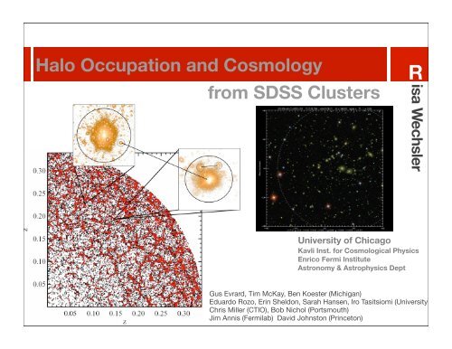
Halo Occupation <strong>and</strong> Cosmology<br />
from SDSS Clusters<br />
<strong>Risa</strong> <strong>Wechsler</strong><br />
University of Chicago<br />
Kavli Inst. for Cosmological Physics<br />
Enrico Fermi Institute<br />
<strong>Astronomy</strong> & <strong>Astrophysics</strong> Dept<br />
Gus Evrard, Tim McKay, Ben Koester (Michigan)<br />
Eduardo Rozo, Erin Sheldon, Sarah Hansen, Iro Tasitsiomi (University of Chic<br />
Chris Miller (CTIO), Bob Nichol (Portsmouth)<br />
Jim Annis (Fermilab) David Johnston (Princeton)
SDSS data now covers >8000 sq<br />
degrees<br />
Cluster finder (maxBCG), uses<br />
photometric data to identify<br />
BCGs <strong>and</strong> red sequence galaxies<br />
More than 800,000 objects with at<br />
least 2 bright red galaxies.<br />
172000 with >=10 bright red<br />
galaxies<br />
dn/dlogN for 0.05
Cluster mass profiles from weak lensing<br />
(the galaxy mass correlation function)<br />
!" [h M O•<br />
pc #2 ]<br />
!" [h M O•<br />
pc #2 ]<br />
!" [h M O•<br />
pc #2 ]<br />
10 4<br />
10 3<br />
10 2<br />
10<br />
1<br />
0.1<br />
10 -2<br />
10 4<br />
10 3<br />
10 2<br />
10<br />
1<br />
0.1<br />
10 -2<br />
10 4<br />
10 3<br />
10 2<br />
10<br />
1<br />
0.1<br />
10 -2<br />
10 -2<br />
1 $ N gals $ 3<br />
8 $ N gals $ 9<br />
31 $ N gals $ 40<br />
0.1 1 10<br />
R [h #1 Mpc]<br />
Sheldon et al 2005 (in prep)<br />
10 -2<br />
4 $ N gals $ 4<br />
10 $ N gals $ 15<br />
41 $ N gals $ 50<br />
0.1 1 10<br />
R [h #1 Mpc]<br />
10 -2<br />
5 $ N gals $ 5<br />
16 $ N gals $ 20<br />
51 $ N gals $ 75<br />
0.1 1 10<br />
R [h #1 Mpc]<br />
10 -2<br />
6 $ N gals $ 7<br />
21 $ N gals $ 30<br />
76 $ N gals $ 343<br />
0.1 1 10<br />
R [h #1 Mpc]<br />
Based on a sample of ~100000 groups (DR3+)
M 200<br />
Lensing Mass<br />
Cluster Size<br />
10 14<br />
10 13<br />
10 12<br />
r 200 [h !1 Mpc]<br />
S<br />
M200 = A Ngal A= 2.1±0.4 ×10 11<br />
S= 1.56±0.07<br />
χ 2 = 11.1 DOF=10<br />
1 10 100<br />
<br />
2.0<br />
1.0<br />
0.9<br />
0.8<br />
0.7<br />
0.6<br />
0.5<br />
Sheldon et al 2005 (in prep)<br />
Hansen et al 2005,<br />
ApJ in press<br />
0.4<br />
6 8 10 20 40 60 80 100<br />
N gals<br />
Sigma diff<br />
Velocity Dispersion<br />
1000<br />
100<br />
Real Data<br />
McKay et al 2005 (in prep)<br />
1 10 100 1000<br />
N gals<br />
several ways to measure the scaling<br />
between cluster richness <strong>and</strong> “mass”<br />
only problem: you don’t know what N is,<br />
<strong>and</strong> you don’t know what M (or sigma or R) is!
M 200<br />
Lensing Mass<br />
r200 [h !1 Cluster Mpc] Size<br />
10 14<br />
10 13<br />
10 12<br />
2.0<br />
1.0<br />
0.9<br />
0.8<br />
0.7<br />
0.6<br />
0.5<br />
S<br />
M200 = A Ngal A= 2.1±0.4 ×10 11<br />
S= 1.56±0.07<br />
χ 2 = 11.1 DOF=10<br />
0.4<br />
6 8 10 20 40 60 80 100<br />
N gals<br />
lensing mass<br />
Sigma diff<br />
1000<br />
several ways to<br />
measure the<br />
scaling between<br />
cluster richness<br />
<strong>and</strong> “mass”<br />
Real Data<br />
• need to underst<strong>and</strong> velocity bias (as a function of radius & L)<br />
1<br />
Sheldon et al 2005 (in prep)<br />
• can measure scatter<br />
10 100<br />
cluster sizes<br />
100<br />
1 10<br />
McKay et al 2005 (in prep)<br />
100 1000<br />
Ngals Hansen et al 2005,<br />
ApJ in press<br />
Velocity Dispersion<br />
• well understood theoretically<br />
• selection biases <strong>and</strong> centering effects need to be understood<br />
• no direct method to measure scatter<br />
cluster velocity dispersions<br />
• need additional data (spectra), which is typically redshift dependent<br />
1000.0<br />
• depends on galaxy background, degenerate with cosmology<br />
cluster-cluster correlation function<br />
• no direct method to measure scatter<br />
ξ(r)<br />
Cluster Correlation<br />
Function<br />
100.0<br />
10.0<br />
• uncertainties in redshifts can bias measurements<br />
probably have more scatter than Lx, SZ,<br />
1.0<br />
but order of magnitude easier to find<br />
0.1<br />
1 10 100<br />
r [Mpc/h]
how to predict cluster observables theoretically?<br />
two-part question:<br />
• how are galaxies connected to dark matter (bias/halo occupation)<br />
• how are clusters observables connected to real groups/clusters of galaxies?<br />
mock catalogs that connect theoretically understood quantities to the full<br />
richness of the SDSS data set:<br />
• need a large simulated volume: would like to have a method that can work<br />
without high resolution simulations<br />
• best cluster finders depend on galaxy luminosity <strong>and</strong> color; need galaxies with<br />
realistic luminosities & colors <strong>and</strong> to match joint luminosity-color distribution as a<br />
function of redshift & local density<br />
• run identical analysis code used on data on simulations<br />
basic method<br />
1. populate the simulation with the measured luminosity function.<br />
2. luminosity dependent bias: assign galaxies to dark matter particles based on<br />
the local dark matter galaxy distribution by tuning P(δ dm |L) to match the<br />
observed luminosity dependent 2-pt. correlation function<br />
3. color based on the luminosity <strong>and</strong> local galaxy density: each mock galaxy gets<br />
assigned a real SDSS galaxy from a volume-limited sample, based on its<br />
luminosity <strong>and</strong> galaxy density
Adding Density Determined GAlaxies to Light-cone Simulations<br />
(ADDGALS)<br />
assign galaxies to dark matter particles<br />
based on their local dark matter, with<br />
some probability P(δm|Mr)<br />
a useful measure of local mass density:<br />
radius enclosing M=M* (~2x10 13 Msun/<br />
h)--for dm, distribution is a lognormal<br />
+gaussian<br />
assume that at every luminosity, the<br />
galaxy population has a local density PDF<br />
with this form, for some choice of<br />
parameters<br />
as a function of luminosity, constrain the<br />
values of the PDF with the two-point<br />
correlation function wp(r, L)<br />
use an MCMC approach to constrain the<br />
five parameters of the distribution as a<br />
function of luminosity<br />
probability<br />
0.6<br />
0.5<br />
0.4<br />
0.3<br />
0.2<br />
0.1<br />
Mr
slope of this fraction R_delta at L*<br />
slope of R_delta<br />
fraction of “field”galaxies<br />
probability<br />
0.6<br />
0.5<br />
0.4<br />
0.3<br />
0.2<br />
0.1<br />
Mr
the recipe<br />
1. populate the simulation with a given luminosity function. was<br />
using SDSS r-b<strong>and</strong> LF with 1.6mag evolution per unit redshift.<br />
(switch to 1.3mag per unit z?)<br />
2. luminosity dependent bias: assign galaxies to dark matter particles<br />
based on the local dark matter galaxy distribution by tuning P<br />
(δ dm |Mr) to match the observed luminosity dependent 2-pt.<br />
correlation function<br />
3. each mock galaxy gets assigned a real SDSS galaxies, based on<br />
its luminosity <strong>and</strong> local galaxy<br />
measure the 5th/10th nearest neighbor galaxy for a volume<br />
limited sample. for 0.4L* (Mr = -19.78), this is ~z=0.05-0.1.<br />
measure this same density estimator for each of the mock<br />
galaxies<br />
bin galaxies in L <strong>and</strong> dg, choose a real galaxy from the<br />
appropriate bin<br />
4. apply simple target selection algorithm, main + LRGs
probability<br />
probability<br />
this mock catalog matches the<br />
data in several key respects<br />
1.2<br />
1.0<br />
0.8<br />
0.6<br />
0.4<br />
M z<br />
M r<br />
M g<br />
M u<br />
0.2<br />
0.0<br />
-23 -22 -21 -20 -19 -18 -17 -16<br />
M-5logh<br />
color distribution & evolution<br />
6<br />
5<br />
4<br />
3<br />
2<br />
1<br />
0<br />
luminosity function & evolution<br />
r-z<br />
g-i<br />
0 1 2 3<br />
color<br />
u-r<br />
!<br />
g-r color<br />
hv_2c_nn4/<br />
1000.0<br />
100.0<br />
10.0<br />
1.0<br />
0.1<br />
!23
halo occupation this method<br />
N gals<br />
100.00<br />
10.00<br />
1.00<br />
0.10<br />
0.01<br />
10 12<br />
M r < -20<br />
subhalo vf (KBW04)<br />
galaxy-mass (TKWP 04)<br />
ξ gg; bias(W05)<br />
ξ gg; CLFWW05<br />
M r
halo occupation: cosmological dependence<br />
fraction of<br />
“field”galaxies<br />
1.0<br />
0.9<br />
0.8<br />
σ 8<br />
0.7<br />
2.0 2.5 3.0 3.5 4.0<br />
denser regions<br />
σ 8<br />
fixed galaxy clustering (now well measured!) + cosmologically dependent dark matter <strong>and</strong> halo<br />
clustering --> changing bias model.<br />
lower normalization + same galaxy clustering -- same galaxies in more massive halos<br />
--> higher halo occupation, same galaxies live in denser regions
First thing to calibrate in the cluster finder:<br />
P(Ngals, obs| Ng, true)<br />
number of galaxies identified by cluster finder<br />
(within 1Mpc)<br />
number of galaxies within Rvir<br />
Turns out the problem is<br />
basically separable into<br />
two parts:<br />
1) for a given cosmology,<br />
how do the galaxies<br />
populate the dark matter?<br />
2) for a given cluster finder,<br />
how does Ntrue relate to<br />
Nobserved?<br />
**not dependent on<br />
cosmology or the relation<br />
between galaxies <strong>and</strong> dark<br />
matter**
cluster abundance alone<br />
number of halos<br />
10000<br />
1000<br />
100<br />
10<br />
10 13<br />
1<br />
10 14<br />
halo mass<br />
σ 8 =0.77, 0.9<br />
10 15<br />
number of clusters<br />
10000<br />
1000<br />
100<br />
10<br />
for ~5000 sq degrees to z~0.3<br />
with cluster richness<br />
as the “mass” measurement<br />
1<br />
10 100<br />
Ngals
M 200<br />
Lensing Mass<br />
Cluster Size<br />
10 14<br />
10 13<br />
10 12<br />
r 200 [h !1 Mpc]<br />
S<br />
M200 = A Ngal A= 2.1±0.4 ×10 11<br />
S= 1.56±0.07<br />
χ 2 = 11.1 DOF=10<br />
Sigma diff<br />
1000<br />
Real Data<br />
Sheldon et al 2005 (in prep) McKay et al 2005 (in prep)<br />
100<br />
1 10 100<br />
<br />
2.0<br />
1.0<br />
0.9<br />
0.8<br />
0.7<br />
0.6<br />
0.5<br />
Hansen et al 2005,<br />
ApJ in press<br />
0.4<br />
6 8 10 20 40 60 80 100<br />
N gals<br />
Velocity Dispersion<br />
1 10 100 1000<br />
N gals<br />
Now we know what the x-axis is.<br />
Since we have realistic clusters, we can now<br />
measure each of the y-axes for these plots in<br />
the same way in the models as they are<br />
measured in the data.<br />
Combining these constraints with the cluster<br />
abundance will provide powerful constraints on<br />
both cosmology <strong>and</strong> the true halo occupation.<br />
This extremely rich data set requires<br />
realistic simulations to make the most of it!
Thanks to S<strong>and</strong>y, Joel & George!