chapter 1 - Bentham Science

Multiplexing Techniques for FBG Sensors Fiber Bragg Grating Sensors 101
Multiplexing optical fiber sensors includes four basic tasks [3]: i) Launching an optical signal into the network having a
suitable power, spectral distribution, polarization and modulation; ii) The detection of the signal which has been coded or
modulated by the sensor element, and sent back to the optoelectronic unit by transmission or reflection; iii) Uniquely
identifying the information corresponding to each sensor in the network, by means of proper addressing, polling and
decoding; iv) The evaluation of the generated optical signals by modulating each sensor with a calibrated electrical signal.
To efficiently design the most appropriate sensor network, it is necessary to take into account different aspects: the
modulation and coding format of the optical signal, the network topology, the inclusion or not of optical
amplification technologies, the decoding method for the received signal, and the type or types of sensors
multiplexed in the same network. Finally, it must be also considered the economic conditions, which would
eventually determine the most appropriate network (see Fig. 3).
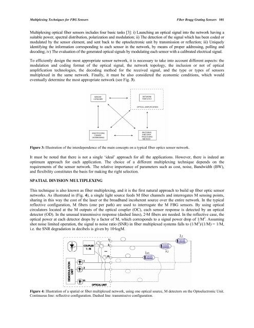
Figure 3: Illustration of the interdependence of the main concepts on a typical fiber optics sensor network.
It must be noted that there is not a single ‘ideal’ approach for all the applications. However, there is indeed an
optimum approach for each application. The choice of a different multiplexing technique depends on the
requirements of the sensor network. The relative importance of parameters such as cost, noise, Bandwidth (BW),
and flexibility constitutes the basis for making the right selection.
SPATIAL DIVISION MULTIPLEXING
This technique is also known as fiber multiplexing, and it is the first natural approach to build up fiber optic sensor
networks. As illustrated in (Fig. 4), a single light source feeds M fiber channels and interrogates M sensing points,
sharing in this way the cost of the laser or the broadband incoherent source over the entire network. In the typical
reflective configuration, M fibers (one per path) are used to interrogate the M FBG sensors. By using optical
circulators located at the M outputs of the optical coupler (OC), each sensor response is detected by an optical
detector (OD). In the unusual transmissive response (dashed lines), 2·M fibers are needed. In the reflective case, the
optical power at each detector drops by a factor of M, which corresponds to a signal power drop of 1/M 2 . Assuming
shot noise limited operation, the signal to noise ratio (SNR) in fiber multiplexed systems falls to (1/M 2 )/(1/M) = 1/M,
i.e. the SNR degradation in decibels is given by 10·logM.
Figure 4: Illustration of a spatial or fiber multiplexed network, using one optical source, M detectors on the Optoelectronic Unit.
Continuous line: reflective configuration. Dashed line: transmissive configuration.