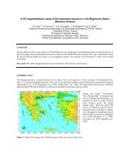
Cave detection using the Self-Potential-Surface (SPS) technique on ...
Cave detection using the Self-Potential-Surface (SPS) technique on ...
Cave detection using the Self-Potential-Surface (SPS) technique on ...

Create successful ePaper yourself
Turn your PDF publications into a flip-book with our unique Google optimized e-Paper software.
19. Kolloquium Elektromagnetische Tiefenforschung, Burg Ludwigstein, 1.10.-5.10.2001, Hrsg.: A. Hördt und J. B. Stoll<br />
<str<strong>on</strong>g>Cave</str<strong>on</strong>g> <str<strong>on</strong>g>detecti<strong>on</strong></str<strong>on</strong>g> <str<strong>on</strong>g>using</str<strong>on</strong>g> <str<strong>on</strong>g>the</str<strong>on</strong>g> <str<strong>on</strong>g>Self</str<strong>on</strong>g>-<str<strong>on</strong>g>Potential</str<strong>on</strong>g>-<str<strong>on</strong>g>Surface</str<strong>on</strong>g> (<str<strong>on</strong>g>SPS</str<strong>on</strong>g>) <str<strong>on</strong>g>technique</str<strong>on</strong>g> <strong>on</strong> a<br />
karstic terrain in <str<strong>on</strong>g>the</str<strong>on</strong>g> Jura mountains (Switzerland)<br />
Marcus Gurk 1,3 , Frank Bosch 2<br />
1 Groupe de Géomagnétisme, Université de Neuchâtel, Switzerland, marcus.gurk@unine.ch<br />
2 Centre D'Hydrogéologie, Université de Neuchâtel, Switzerland, frank.bosch@unine.ch<br />
1 Introducti<strong>on</strong><br />
Originally, Aubert & Atangana (1996)<br />
developed <str<strong>on</strong>g>the</str<strong>on</strong>g> <str<strong>on</strong>g>Self</str<strong>on</strong>g>-<str<strong>on</strong>g>Potential</str<strong>on</strong>g>-<str<strong>on</strong>g>Surface</str<strong>on</strong>g> (<str<strong>on</strong>g>SPS</str<strong>on</strong>g>)<br />
<str<strong>on</strong>g>technique</str<strong>on</strong>g> for hydrogeological explorati<strong>on</strong> of<br />
volcanic areas. Provided that two c<strong>on</strong>diti<strong>on</strong>s<br />
are satisfied, <str<strong>on</strong>g>the</str<strong>on</strong>g>y experimentally found a<br />
linear relati<strong>on</strong> between <str<strong>on</strong>g>the</str<strong>on</strong>g> range of negative<br />
<str<strong>on</strong>g>Self</str<strong>on</strong>g>-<str<strong>on</strong>g>Potential</str<strong>on</strong>g> (SP) anomalies and <str<strong>on</strong>g>the</str<strong>on</strong>g><br />
thickness of <str<strong>on</strong>g>the</str<strong>on</strong>g> unsaturated z<strong>on</strong>e. The first<br />
c<strong>on</strong>diti<strong>on</strong> is a str<strong>on</strong>g c<strong>on</strong>trast between <str<strong>on</strong>g>the</str<strong>on</strong>g><br />
resistivity of <str<strong>on</strong>g>the</str<strong>on</strong>g> unsaturated z<strong>on</strong>e and <str<strong>on</strong>g>the</str<strong>on</strong>g><br />
resistivity of <str<strong>on</strong>g>the</str<strong>on</strong>g> substratum and <str<strong>on</strong>g>the</str<strong>on</strong>g> watersaturated<br />
z<strong>on</strong>e. The sec<strong>on</strong>d c<strong>on</strong>diti<strong>on</strong> is <str<strong>on</strong>g>the</str<strong>on</strong>g><br />
homogeneity of <str<strong>on</strong>g>the</str<strong>on</strong>g> unsaturated z<strong>on</strong>e. The<br />
qualitative interpretati<strong>on</strong> of SP maps<br />
indicates that <str<strong>on</strong>g>the</str<strong>on</strong>g> lines of maximum negative<br />
values corresp<strong>on</strong>d to <str<strong>on</strong>g>the</str<strong>on</strong>g> drainage axes and<br />
<str<strong>on</strong>g>the</str<strong>on</strong>g> lines of minimum negative values to <str<strong>on</strong>g>the</str<strong>on</strong>g><br />
boundaries between two watersheds (Jacks<strong>on</strong><br />
& Kauahikaua (1987)).<br />
We expected similar c<strong>on</strong>diti<strong>on</strong>s to be valid in<br />
carb<strong>on</strong>ate aquifers. Especially in a karstic cave, <str<strong>on</strong>g>the</str<strong>on</strong>g> resistivity c<strong>on</strong>trast created by <str<strong>on</strong>g>the</str<strong>on</strong>g> air-layer must be<br />
significant, so that <str<strong>on</strong>g>the</str<strong>on</strong>g> <str<strong>on</strong>g>SPS</str<strong>on</strong>g> <str<strong>on</strong>g>technique</str<strong>on</strong>g> can be used to detect <str<strong>on</strong>g>the</str<strong>on</strong>g>se structures.<br />
Motivated by this hypo<str<strong>on</strong>g>the</str<strong>on</strong>g>sis, an experiment was c<strong>on</strong>ducted in co-work with <str<strong>on</strong>g>the</str<strong>on</strong>g> Centre of<br />
Hydrogeology Neuchâtel (CHYN).<br />
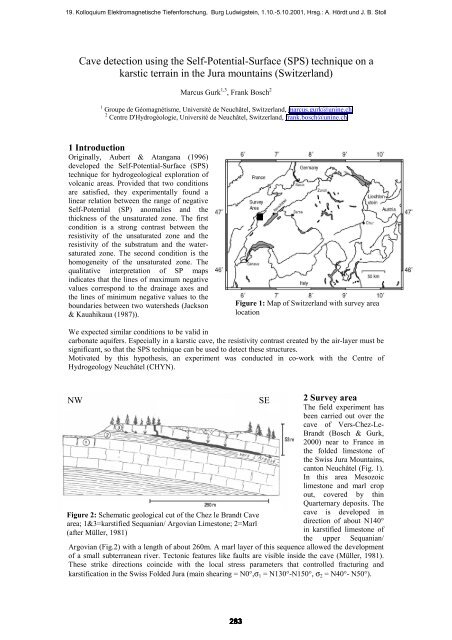
NW SE<br />
Figure 2: Schematic geological cut of <str<strong>on</strong>g>the</str<strong>on</strong>g> Chez le Brandt <str<strong>on</strong>g>Cave</str<strong>on</strong>g><br />
area; 1&3=karstified Sequanian/ Argovian Limest<strong>on</strong>e; 2=Marl<br />
(after Müller, 1981)<br />
Figure 1: Map of Switzerland with survey area<br />
locati<strong>on</strong><br />
2 Survey area<br />
The field experiment has<br />
been carried out over <str<strong>on</strong>g>the</str<strong>on</strong>g><br />
cave of Vers-Chez-Le-<br />
Brandt (Bosch & Gurk,<br />
2000) near to France in<br />
<str<strong>on</strong>g>the</str<strong>on</strong>g> folded limest<strong>on</strong>e of<br />
<str<strong>on</strong>g>the</str<strong>on</strong>g> Swiss Jura Mountains,<br />
cant<strong>on</strong> Neuchâtel (Fig. 1).<br />
In this area Mesozoic<br />
limest<strong>on</strong>e and marl crop<br />
out, covered by thin<br />
Quarternary deposits. The<br />
cave is developed in<br />
directi<strong>on</strong> of about N140°<br />
in karstified limest<strong>on</strong>e of<br />
<str<strong>on</strong>g>the</str<strong>on</strong>g> upper Sequanian/<br />
Argovian (Fig.2) with a length of about 260m. A marl layer of this sequence allowed <str<strong>on</strong>g>the</str<strong>on</strong>g> development<br />
of a small subterranean river. Tect<strong>on</strong>ic features like faults are visible inside <str<strong>on</strong>g>the</str<strong>on</strong>g> cave (Müller, 1981).<br />
These strike directi<strong>on</strong>s coincide with <str<strong>on</strong>g>the</str<strong>on</strong>g> local stress parameters that c<strong>on</strong>trolled fracturing and<br />
karstificati<strong>on</strong> in <str<strong>on</strong>g>the</str<strong>on</strong>g> Swiss Folded Jura (main shearing = N0°,σ1 = N130°-N150°, σ2 = N40°- N50°).
19. Kolloquium Elektromagnetische Tiefenforschung, Burg Ludwigstein, 1.10.-5.10.2001, Hrsg.: A. Hördt und J. B. Stoll<br />
3 <str<strong>on</strong>g>SPS</str<strong>on</strong>g> method<br />
Figure 3a represents <str<strong>on</strong>g>the</str<strong>on</strong>g> <str<strong>on</strong>g>SPS</str<strong>on</strong>g> model for a subhoriz<strong>on</strong>tal layered structure in karst. According to Aubert<br />
et al. (1990) and Aubert & Atangana (1996), three specific c<strong>on</strong>diti<strong>on</strong>s shall be satisfied in this model:<br />
1) A high ratio between <str<strong>on</strong>g>the</str<strong>on</strong>g> resistivity of <str<strong>on</strong>g>the</str<strong>on</strong>g> unsaturated z<strong>on</strong>e (A) and <str<strong>on</strong>g>the</str<strong>on</strong>g> resistivity of <str<strong>on</strong>g>the</str<strong>on</strong>g><br />
impermeable z<strong>on</strong>e (B)<br />
2) Z<strong>on</strong>e (A) is composed out of porous and homogenous medium<br />
3) The resistivity distributi<strong>on</strong> of z<strong>on</strong>e (A) is homogenous<br />
The interface (C) is <str<strong>on</strong>g>the</str<strong>on</strong>g> c<strong>on</strong>tact between z<strong>on</strong>e (A) and z<strong>on</strong>e (B). Under <str<strong>on</strong>g>the</str<strong>on</strong>g> above menti<strong>on</strong>ed c<strong>on</strong>diti<strong>on</strong>s,<br />
Aubert et al. (1990) and Aubert & Atangana (1996) give <str<strong>on</strong>g>the</str<strong>on</strong>g> following experimental linear relati<strong>on</strong>:<br />
V(<br />
x,<br />
y)<br />
d(<br />
x y)<br />
= + d°<br />
K<br />
, (1)<br />
d ( x,<br />
y)<br />
is <str<strong>on</strong>g>the</str<strong>on</strong>g> thickness of <str<strong>on</strong>g>the</str<strong>on</strong>g> unsaturated z<strong>on</strong>e (A) and V( x,<br />
y)<br />
is <str<strong>on</strong>g>the</str<strong>on</strong>g> range of SP anomaly measured at<br />
<str<strong>on</strong>g>the</str<strong>on</strong>g> surface.<br />
K is a coefficient in Volt/Meter, E° is <str<strong>on</strong>g>the</str<strong>on</strong>g> known thickness of z<strong>on</strong>e (A) below <str<strong>on</strong>g>the</str<strong>on</strong>g> SP reference point<br />
R, where V ( R)<br />
= 0 Volt by c<strong>on</strong>venti<strong>on</strong>.<br />
The interface (C) would <str<strong>on</strong>g>the</str<strong>on</strong>g>n be an equipotential surface, called <str<strong>on</strong>g>the</str<strong>on</strong>g> <str<strong>on</strong>g>Self</str<strong>on</strong>g>-<str<strong>on</strong>g>Potential</str<strong>on</strong>g>-<str<strong>on</strong>g>Surface</str<strong>on</strong>g> (<str<strong>on</strong>g>SPS</str<strong>on</strong>g>).<br />
K is a functi<strong>on</strong> of various parameters including <str<strong>on</strong>g>the</str<strong>on</strong>g> average resistivity of z<strong>on</strong>e (A) and <str<strong>on</strong>g>the</str<strong>on</strong>g> resistivity of<br />
z<strong>on</strong>e (B). When <str<strong>on</strong>g>the</str<strong>on</strong>g> <str<strong>on</strong>g>SPS</str<strong>on</strong>g> is sub-horiz<strong>on</strong>tal, K defines <str<strong>on</strong>g>the</str<strong>on</strong>g> topographic effect in SP and we can derive<br />
K by:<br />
dV<br />
K = , (2)<br />
dh<br />
i.e. by <str<strong>on</strong>g>the</str<strong>on</strong>g> vertical SP gradient from <str<strong>on</strong>g>the</str<strong>on</strong>g> reference point R down to <str<strong>on</strong>g>the</str<strong>on</strong>g> surface of z<strong>on</strong>e (B):<br />
dV(<br />
R )<br />
K = , (3)<br />
d°<br />
K can be determined from borehole informati<strong>on</strong> or laboratory measurements of rock samples of z<strong>on</strong>e<br />
(A).<br />
If <str<strong>on</strong>g>the</str<strong>on</strong>g> field topography ( x y)<br />
topography of <str<strong>on</strong>g>the</str<strong>on</strong>g> <str<strong>on</strong>g>SPS</str<strong>on</strong>g>:<br />
h , and <str<strong>on</strong>g>the</str<strong>on</strong>g> SP mapping ( x,<br />
y)<br />
V are known, we can <str<strong>on</strong>g>the</str<strong>on</strong>g>n calculate <str<strong>on</strong>g>the</str<strong>on</strong>g><br />
V(<br />
x,<br />
y)<br />
H(<br />
x,<br />
y)<br />
= h(<br />
x,<br />
y)<br />
− d°<br />
−<br />
(4)<br />
K<br />
The <str<strong>on</strong>g>SPS</str<strong>on</strong>g> topography will give <str<strong>on</strong>g>the</str<strong>on</strong>g> topography of <str<strong>on</strong>g>the</str<strong>on</strong>g> impermeable z<strong>on</strong>e (B).<br />
A cave will significantly change <str<strong>on</strong>g>the</str<strong>on</strong>g> potential distributi<strong>on</strong> in <str<strong>on</strong>g>the</str<strong>on</strong>g> structure and <str<strong>on</strong>g>the</str<strong>on</strong>g>refore <str<strong>on</strong>g>the</str<strong>on</strong>g> SP mapping<br />
at surface. In our working model for <str<strong>on</strong>g>the</str<strong>on</strong>g> field experiment (Fig. 3b), a possible equipotential surface is<br />
thought to align with <str<strong>on</strong>g>the</str<strong>on</strong>g> bottom of <str<strong>on</strong>g>the</str<strong>on</strong>g> cave. Ano<str<strong>on</strong>g>the</str<strong>on</strong>g>r possible equipotential surface can be c<strong>on</strong>sidered<br />
to follow <str<strong>on</strong>g>the</str<strong>on</strong>g> roof of <str<strong>on</strong>g>the</str<strong>on</strong>g> cave.
19. Kolloquium Elektromagnetische Tiefenforschung, Burg Ludwigstein, 1.10.-5.10.2001, Hrsg.: A. Hördt und J. B. Stoll<br />
Figure 4: <str<strong>on</strong>g>Self</str<strong>on</strong>g>-<str<strong>on</strong>g>Potential</str<strong>on</strong>g><br />
equipment "Type Münster"<br />
Figure 3a: <str<strong>on</strong>g>SPS</str<strong>on</strong>g> model for a subhoriz<strong>on</strong>tal<br />
layered structure in karst<br />
Figure 3b: <str<strong>on</strong>g>SPS</str<strong>on</strong>g> model for a subhoriz<strong>on</strong>tal<br />
layered structure in karst with<br />
a cave<br />
4 Field experiment<br />
The experiment was carried out over a<br />
shallow part (depth between 5 to 12 m)<br />
of <str<strong>on</strong>g>the</str<strong>on</strong>g> cave (Fig. 5).<br />
Positi<strong>on</strong>ing of <str<strong>on</strong>g>the</str<strong>on</strong>g> reference Electrode<br />
Besides <str<strong>on</strong>g>the</str<strong>on</strong>g> careful sampling of <str<strong>on</strong>g>the</str<strong>on</strong>g> SP<br />
anomalies, <str<strong>on</strong>g>the</str<strong>on</strong>g> accurate estimate of K is<br />
crucial for <str<strong>on</strong>g>the</str<strong>on</strong>g> method. One of <str<strong>on</strong>g>the</str<strong>on</strong>g> main<br />
problems in a cave is to determine<br />
E° and <str<strong>on</strong>g>the</str<strong>on</strong>g> plumb line between <str<strong>on</strong>g>the</str<strong>on</strong>g> SP<br />
reference point R to <str<strong>on</strong>g>the</str<strong>on</strong>g> vertical<br />
electrode inside <str<strong>on</strong>g>the</str<strong>on</strong>g> cave. d° must be<br />
taken from maps and crosscuts.<br />
To delineate <str<strong>on</strong>g>the</str<strong>on</strong>g> projecti<strong>on</strong> of <str<strong>on</strong>g>the</str<strong>on</strong>g><br />
positi<strong>on</strong> of <str<strong>on</strong>g>the</str<strong>on</strong>g> vertical electrode (placed<br />
inside <str<strong>on</strong>g>the</str<strong>on</strong>g> cave) to <str<strong>on</strong>g>the</str<strong>on</strong>g> surface we now<br />
use a triangulati<strong>on</strong> method:<br />
At <str<strong>on</strong>g>the</str<strong>on</strong>g> chosen positi<strong>on</strong> of <str<strong>on</strong>g>the</str<strong>on</strong>g> vertical<br />
electrode in <str<strong>on</strong>g>the</str<strong>on</strong>g> cave we set up a<br />
portable VLF transmitter of 13.5 kHz<br />
(Fig. 6) and triangulating its projecti<strong>on</strong><br />
to <str<strong>on</strong>g>the</str<strong>on</strong>g> surface with <str<strong>on</strong>g>the</str<strong>on</strong>g> RMT<br />
(RadiofrequencyMagnetoTelluric)<br />
equipment (Fig. 7) developed at CHYN.<br />
This method will give <str<strong>on</strong>g>the</str<strong>on</strong>g> positi<strong>on</strong> R for<br />
<str<strong>on</strong>g>the</str<strong>on</strong>g> reference electrode of <str<strong>on</strong>g>the</str<strong>on</strong>g> SP<br />
mapping at <str<strong>on</strong>g>the</str<strong>on</strong>g> surface (Fig. 3a and 3b).<br />
Vertical SP gradient (K)<br />
Estimates of K were obtained by placing an electrode in <str<strong>on</strong>g>the</str<strong>on</strong>g> bottom of <str<strong>on</strong>g>the</str<strong>on</strong>g><br />
cave (z<strong>on</strong>e (B)) beneath reference point R and sampling <str<strong>on</strong>g>the</str<strong>on</strong>g> vertical SP<br />
gradient between this electrode and <str<strong>on</strong>g>the</str<strong>on</strong>g> reference electrode at <str<strong>on</strong>g>the</str<strong>on</strong>g> surface.<br />
K was found in this experiment to be –10.3 mV/15m.<br />
Topography and SP mapping at <str<strong>on</strong>g>the</str<strong>on</strong>g> surface<br />
We sampled topographic and SP data at <str<strong>on</strong>g>the</str<strong>on</strong>g> surface in a 10m x 20m area (x -><br />
East, y-> South). SP data were collected every meter <str<strong>on</strong>g>using</str<strong>on</strong>g> saturated Cu-<br />
CuSO4 electrodes arranged <strong>on</strong> a spade stick (Fig. 4). All SP values are<br />
sampled in addicti<strong>on</strong> to <str<strong>on</strong>g>the</str<strong>on</strong>g> surface reference electrode at positi<strong>on</strong> R.
19. Kolloquium Elektromagnetische Tiefenforschung, Burg Ludwigstein, 1.10.-5.10.2001, Hrsg.: A. Hördt und J. B. Stoll<br />
Figure 5: The experiment site and part of <str<strong>on</strong>g>the</str<strong>on</strong>g> cave Vers-Chez-Le-Brandt<br />
Figure 6 (left): Portable VLF transmitter (grey box) of 13.5 kHz <strong>on</strong> <str<strong>on</strong>g>the</str<strong>on</strong>g> bottom of <str<strong>on</strong>g>the</str<strong>on</strong>g> cave, <str<strong>on</strong>g>the</str<strong>on</strong>g> vertical<br />
electrode will be placed in <str<strong>on</strong>g>the</str<strong>on</strong>g> centre of <str<strong>on</strong>g>the</str<strong>on</strong>g> rectangular coil<br />
Figure 7 (right): CHYN’s RMT receiver and horiz<strong>on</strong>tal coil above <str<strong>on</strong>g>the</str<strong>on</strong>g> cave to triangulate <str<strong>on</strong>g>the</str<strong>on</strong>g><br />
projecti<strong>on</strong> of <str<strong>on</strong>g>the</str<strong>on</strong>g> transmitter positi<strong>on</strong> to <str<strong>on</strong>g>the</str<strong>on</strong>g> surface. This will give <str<strong>on</strong>g>the</str<strong>on</strong>g> SP reference point R .<br />
5 Results<br />
The findings of <str<strong>on</strong>g>the</str<strong>on</strong>g> experiment are presented in Figure 8. First of all we find that <str<strong>on</strong>g>the</str<strong>on</strong>g> SP-mapping is decoupled<br />
from <str<strong>on</strong>g>the</str<strong>on</strong>g> surface topography, indicating that <str<strong>on</strong>g>the</str<strong>on</strong>g> SP is created by internal features of <str<strong>on</strong>g>the</str<strong>on</strong>g><br />
subsoil. The SP data varies between values of –8 to +4 mV, which is found to be a typical range for SP<br />
data <strong>on</strong> karst areas in <str<strong>on</strong>g>the</str<strong>on</strong>g> Jura mountain (Bosch & Gurk, 2000). The SP mapping itself allows drawing<br />
c<strong>on</strong>clusi<strong>on</strong> about <str<strong>on</strong>g>the</str<strong>on</strong>g> positi<strong>on</strong> of <str<strong>on</strong>g>the</str<strong>on</strong>g> cave: Maximum negative SP values at y = 20-28m are indicating<br />
<str<strong>on</strong>g>the</str<strong>on</strong>g> main cave and main drainage axis to be East – Sou<str<strong>on</strong>g>the</str<strong>on</strong>g>ast with a branch (minimum negative values)<br />
that leads towards <str<strong>on</strong>g>the</str<strong>on</strong>g> North.<br />
However, <str<strong>on</strong>g>the</str<strong>on</strong>g> valence of <str<strong>on</strong>g>the</str<strong>on</strong>g> SP data with <str<strong>on</strong>g>the</str<strong>on</strong>g> topographic informati<strong>on</strong> and <str<strong>on</strong>g>the</str<strong>on</strong>g> vertical SP gradient (K)<br />
gives a detailed view insight <str<strong>on</strong>g>the</str<strong>on</strong>g> cave’s topography. The estimate of d ° and K was sufficient to give a<br />
comparable topography of <str<strong>on</strong>g>the</str<strong>on</strong>g> bottom of <str<strong>on</strong>g>the</str<strong>on</strong>g> cave (Fig. 9).
19. Kolloquium Elektromagnetische Tiefenforschung, Burg Ludwigstein, 1.10.-5.10.2001, Hrsg.: A. Hördt und J. B. Stoll<br />
Figure 8: Topography, SP-mapping and <str<strong>on</strong>g>the</str<strong>on</strong>g> resulting <str<strong>on</strong>g>SPS</str<strong>on</strong>g> over <str<strong>on</strong>g>the</str<strong>on</strong>g> cave Vers-Chez-Le-Brandt.<br />
For spatial positi<strong>on</strong> of <str<strong>on</strong>g>the</str<strong>on</strong>g> survey see Fig. 5 (x-> East, y -> South).
19. Kolloquium Elektromagnetische Tiefenforschung, Burg Ludwigstein, 1.10.-5.10.2001, Hrsg.: A. Hördt und J. B. Stoll<br />
Figure 9: Comparis<strong>on</strong> of <str<strong>on</strong>g>SPS</str<strong>on</strong>g> slices of Fig 8 (x=<br />
1,2, …,10, blue, respectively thin lines) and its<br />
visual average (red, respectively thick line) with <str<strong>on</strong>g>the</str<strong>on</strong>g><br />
crosscut based <strong>on</strong> speological data of <str<strong>on</strong>g>the</str<strong>on</strong>g> cave taken<br />
from Fig. 5.<br />
6 Discussi<strong>on</strong><br />
By definiti<strong>on</strong>, <str<strong>on</strong>g>the</str<strong>on</strong>g> <str<strong>on</strong>g>SPS</str<strong>on</strong>g> <str<strong>on</strong>g>technique</str<strong>on</strong>g> does not account<br />
for any inhomogeneities, such as a cave.<br />
Theoretically, <str<strong>on</strong>g>the</str<strong>on</strong>g> method should have failed.<br />
However, to explain our experimental observati<strong>on</strong><br />
at surface we divide <str<strong>on</strong>g>the</str<strong>on</strong>g> problem into an active and<br />
static part. The active part comprises <str<strong>on</strong>g>the</str<strong>on</strong>g><br />
mechanism that creates a charge accumulati<strong>on</strong> al<strong>on</strong>g<br />
<str<strong>on</strong>g>the</str<strong>on</strong>g> <str<strong>on</strong>g>SPS</str<strong>on</strong>g>, whereas <str<strong>on</strong>g>the</str<strong>on</strong>g> passive part explains how this<br />
charge distributi<strong>on</strong> is mirrored to <str<strong>on</strong>g>the</str<strong>on</strong>g> surface. The<br />
latter questi<strong>on</strong> can be qualitatively explained in<br />
terms of a capacitor with various dielectric media:<br />
Static model for a subhoriz<strong>on</strong>tal layered structure<br />
without a cave<br />
We state that <str<strong>on</strong>g>the</str<strong>on</strong>g> K factor, as defined in <str<strong>on</strong>g>the</str<strong>on</strong>g> original<br />
idea by Aubert et al. (1990) and Aubert & Atangana<br />
(1996) for a subhoriz<strong>on</strong>tal layered structure of<br />
homogenious media, is similar to <str<strong>on</strong>g>the</str<strong>on</strong>g> electric field<br />
strength in a capacitor (Fig. 10 a)):<br />
EF ≅ K . (5)<br />
E F electrical field strength<br />
A area<br />
Q charge<br />
D displacement of charge<br />
d distance<br />
ε 0 electrical permittivity of vacuum<br />
1 −9<br />
As<br />
( 10 )<br />
36π<br />
Vm<br />
ε r relative electrical permittivity<br />
( ε lim est<strong>on</strong>e = 8 – 12, ε water = 80, ε air =1)<br />
V potential<br />
(Values taken from Landolt & Börnstein<br />
(1952))<br />
Figure 10: a) Capacitor without and b) capacitor with a dielectric media. c) Capacitor with a series of<br />
dielectric media.
19. Kolloquium Elektromagnetische Tiefenforschung, Burg Ludwigstein, 1.10.-5.10.2001, Hrsg.: A. Hördt und J. B. Stoll<br />
For a given charge distributi<strong>on</strong><br />
r F E D<br />
Q<br />
= = ε 0ε<br />
, (6)<br />
A<br />
<str<strong>on</strong>g>the</str<strong>on</strong>g> electric field strength is defined as:<br />
E<br />
F<br />
V(<br />
x,<br />
y)<br />
= (7)<br />
d ( x,<br />
y)<br />
From this equati<strong>on</strong> we obtain <str<strong>on</strong>g>the</str<strong>on</strong>g> potential:<br />
( x,<br />
y)<br />
= E F ⋅ d ( x y)<br />
, respectively V ( x,<br />
y)<br />
= K ⋅ d ( x,<br />
y)<br />
. (8)<br />
V ,<br />
Similar to a capacitor, <str<strong>on</strong>g>the</str<strong>on</strong>g> charge <strong>on</strong> its boundaries is depending <strong>on</strong> <str<strong>on</strong>g>the</str<strong>on</strong>g> polarisati<strong>on</strong> effect in a given<br />
dielectric medium between <str<strong>on</strong>g>the</str<strong>on</strong>g>se boundaries. In a carb<strong>on</strong>ate aquifer, <str<strong>on</strong>g>the</str<strong>on</strong>g> electrical permittivity of<br />
limest<strong>on</strong>e enhances <str<strong>on</strong>g>the</str<strong>on</strong>g> charge by a factor 8 – 12:<br />
Q<br />
= D = ε 0ε lim est<strong>on</strong>e K<br />
(9)<br />
A<br />
With<br />
D<br />
K = we get a measure for <str<strong>on</strong>g>the</str<strong>on</strong>g> thickness of <str<strong>on</strong>g>the</str<strong>on</strong>g> structure:<br />
ε 0ε lim est<strong>on</strong>e<br />
V(<br />
x,<br />
y)<br />
( x,<br />
y)<br />
= ε 0ε<br />
est<strong>on</strong>e . (10)<br />
D<br />
d lim<br />
And <str<strong>on</strong>g>the</str<strong>on</strong>g> potential is given by:<br />
V<br />
( x,<br />
y)<br />
d ( x,<br />
y)<br />
= D . (11)<br />
ε ε<br />
0 lim est<strong>on</strong>e<br />
Static model for a subhoriz<strong>on</strong>tal layered structure with a cave and water<br />
This model is characterised by a series of capacitors with different dielectric media:<br />
D ε<br />
1 0 1 F 1 E ε = , 2 0 2 F 2 E D ε ε<br />
= , …, Di = ε 0ε i2<br />
EF<br />
i<br />
(12)<br />
Since <str<strong>on</strong>g>the</str<strong>on</strong>g> charge distributi<strong>on</strong> at <str<strong>on</strong>g>the</str<strong>on</strong>g> boundaries are equal:<br />
D D Di<br />
D = =<br />
1 = 2 ... . (13)<br />
The resulting potential of a multiple layered structure is:<br />
D ⎛ d1<br />
d 2 di<br />
⎞ D d i<br />
V(<br />
′ x,<br />
y)<br />
= ⎜<br />
⎟<br />
⎜<br />
+ + ... +<br />
⎟<br />
= ∑ . (14)<br />
ε 0 ⎝ ε1<br />
ε 2 ε i ⎠ ε 0 ε i<br />
To estimate <str<strong>on</strong>g>the</str<strong>on</strong>g> effect of <str<strong>on</strong>g>the</str<strong>on</strong>g>se structures <strong>on</strong> our field experiment, we calculate <str<strong>on</strong>g>the</str<strong>on</strong>g> resulting potential<br />
for three specific models (Figure 11):<br />
Model A: limest<strong>on</strong>e<br />
D ⎛ d1<br />
⎞<br />
V( ′ x , y)<br />
=<br />
⎜<br />
⎟ , 1 8<br />
ε 0 ⎝ ε1<br />
⎠<br />
= ε , (15)
19. Kolloquium Elektromagnetische Tiefenforschung, Burg Ludwigstein, 1.10.-5.10.2001, Hrsg.: A. Hördt und J. B. Stoll<br />
Model B: limest<strong>on</strong>e and air<br />
D ⎛ d1<br />
d 2 ⎞<br />
V( ′ x , y)<br />
=<br />
⎜ +<br />
⎟ , ε1 = 8, d 1 = 5m,<br />
ε 2 = 1,<br />
ε 0 ⎝ ε1<br />
ε 2 ⎠<br />
(16)<br />
Model C: limest<strong>on</strong>e, air and water<br />
D ⎛ d<br />
⎞<br />
⎜ 1 d 2 d3<br />
V( ′ x , y)<br />
=<br />
⎟<br />
⎜<br />
+ +<br />
⎟<br />
, ε1 = 8, d 1 = 5m,<br />
ε 2 = 1,<br />
d 2 = 10m,<br />
ε 3 = 80.<br />
ε 0 ⎝ ε1<br />
ε 2 ε 3 ⎠<br />
(17)<br />
For <str<strong>on</strong>g>the</str<strong>on</strong>g> calculati<strong>on</strong> we used <str<strong>on</strong>g>the</str<strong>on</strong>g> experimental estimate of <str<strong>on</strong>g>the</str<strong>on</strong>g> electric displacement D = Kε<br />
0ε lim est<strong>on</strong>e .<br />
Figure 11: The resulting potential V for three specific layered capacitor models.<br />
Model A is a <strong>on</strong>e-layer structure c<strong>on</strong>sisting solely of limest<strong>on</strong>e with increasing thickness. Figure 11<br />
shows that this limest<strong>on</strong>e layer will have a measurable effect <strong>on</strong> <str<strong>on</strong>g>the</str<strong>on</strong>g> potential distributi<strong>on</strong> at surface<br />
with a beginning thickness of some meters.<br />
In Model B, we kept <str<strong>on</strong>g>the</str<strong>on</strong>g> thickness of <str<strong>on</strong>g>the</str<strong>on</strong>g> limest<strong>on</strong>e roof c<strong>on</strong>stant (5m) and inserted a cavity (air) of<br />
varying thickness. This will enhance <str<strong>on</strong>g>the</str<strong>on</strong>g> measurable effect <strong>on</strong> <str<strong>on</strong>g>the</str<strong>on</strong>g> potential distributi<strong>on</strong> at surface.<br />
The str<strong>on</strong>gest effect <strong>on</strong> <str<strong>on</strong>g>the</str<strong>on</strong>g> potential distributi<strong>on</strong> is shown in Model C. Here, we studied <str<strong>on</strong>g>the</str<strong>on</strong>g> wetting<br />
effect of a (thin) water layer at <str<strong>on</strong>g>the</str<strong>on</strong>g> bottom or at <str<strong>on</strong>g>the</str<strong>on</strong>g> roof of a given cave (roof out of limest<strong>on</strong>e 5m<br />
thick, cavity (air) 10m thick). As Figure 11 shows, a thin water layer affects <str<strong>on</strong>g>the</str<strong>on</strong>g> measurable potential<br />
distributi<strong>on</strong> at surface enormously.<br />
From <str<strong>on</strong>g>the</str<strong>on</strong>g>se simple models we can c<strong>on</strong>clude, that an air layer and <str<strong>on</strong>g>the</str<strong>on</strong>g> wetting effect of water will locally<br />
affect <str<strong>on</strong>g>the</str<strong>on</strong>g> SP values at <str<strong>on</strong>g>the</str<strong>on</strong>g> surface. Hence, <str<strong>on</strong>g>the</str<strong>on</strong>g> cave is detectable with <str<strong>on</strong>g>the</str<strong>on</strong>g> SP <str<strong>on</strong>g>technique</str<strong>on</strong>g>.<br />
Compared to <str<strong>on</strong>g>the</str<strong>on</strong>g> model by Aubert et al. (1990) and Aubert & Atangana (1996) our capacitor model is<br />
independent from <str<strong>on</strong>g>the</str<strong>on</strong>g> resistivities of Z<strong>on</strong>e (A) and (B). In analogy to <str<strong>on</strong>g>the</str<strong>on</strong>g> geo-battery model for large SP<br />
anomalies created by geochemical processes (Bigalke & Grabner, 1997) we term our static model a<br />
geo-capacitor model.
19. Kolloquium Elektromagnetische Tiefenforschung, Burg Ludwigstein, 1.10.-5.10.2001, Hrsg.: A. Hördt und J. B. Stoll<br />
Active model<br />
Superimposed <strong>on</strong> <str<strong>on</strong>g>the</str<strong>on</strong>g> static charge distributi<strong>on</strong> we assume an active charge separati<strong>on</strong> that is c<strong>on</strong>trolled<br />
by <str<strong>on</strong>g>the</str<strong>on</strong>g> (micro) climatic c<strong>on</strong>diti<strong>on</strong>s in <str<strong>on</strong>g>the</str<strong>on</strong>g> cave. For shallow cavities, heat and water transport by<br />
oscillatory c<strong>on</strong>vecti<strong>on</strong> plays an important role (Morat et al., 1999). Periodical variati<strong>on</strong>s of <str<strong>on</strong>g>the</str<strong>on</strong>g><br />
temperature, relatively humidity, air pressure and <str<strong>on</strong>g>the</str<strong>on</strong>g> <str<strong>on</strong>g>Self</str<strong>on</strong>g>-<str<strong>on</strong>g>Potential</str<strong>on</strong>g> (at <str<strong>on</strong>g>the</str<strong>on</strong>g> roof of <str<strong>on</strong>g>the</str<strong>on</strong>g> cave !) are<br />
interpreted as manifestati<strong>on</strong>s of oscillatory c<strong>on</strong>vecti<strong>on</strong> moti<strong>on</strong>s of <str<strong>on</strong>g>the</str<strong>on</strong>g> air inside <str<strong>on</strong>g>the</str<strong>on</strong>g> cave, driven by <str<strong>on</strong>g>the</str<strong>on</strong>g><br />
geo<str<strong>on</strong>g>the</str<strong>on</strong>g>rmal gradient and transporting water as well as heat from <str<strong>on</strong>g>the</str<strong>on</strong>g> bottom to <str<strong>on</strong>g>the</str<strong>on</strong>g> roof.<br />
Morat (1999) state that c<strong>on</strong>vecti<strong>on</strong> is a much more efficient mechanism of heat transport than<br />
c<strong>on</strong>ducti<strong>on</strong> through <str<strong>on</strong>g>the</str<strong>on</strong>g> air of <str<strong>on</strong>g>the</str<strong>on</strong>g> cavity. The air will c<strong>on</strong>vect and transport heat, but, at <str<strong>on</strong>g>the</str<strong>on</strong>g> same time,<br />
it will entrain upward <str<strong>on</strong>g>the</str<strong>on</strong>g> water vapour released at <str<strong>on</strong>g>the</str<strong>on</strong>g> floor of <str<strong>on</strong>g>the</str<strong>on</strong>g> cave by evaporati<strong>on</strong>. The vapour will<br />
c<strong>on</strong>dense <strong>on</strong> <str<strong>on</strong>g>the</str<strong>on</strong>g> roof and <str<strong>on</strong>g>the</str<strong>on</strong>g> upper part of <str<strong>on</strong>g>the</str<strong>on</strong>g> pillars. In general, <str<strong>on</strong>g>the</str<strong>on</strong>g> c<strong>on</strong>densed water enters <str<strong>on</strong>g>the</str<strong>on</strong>g> rock<br />
by capillarity, and <str<strong>on</strong>g>the</str<strong>on</strong>g> relative humidity of <str<strong>on</strong>g>the</str<strong>on</strong>g> air remains c<strong>on</strong>stant in <str<strong>on</strong>g>the</str<strong>on</strong>g> cave. This aspect toge<str<strong>on</strong>g>the</str<strong>on</strong>g>r<br />
with <str<strong>on</strong>g>the</str<strong>on</strong>g> streaming potential in <str<strong>on</strong>g>the</str<strong>on</strong>g> porous media of z<strong>on</strong>e (A) (Revil et al., 1999a, Revil et al., 1999b)<br />
plays an important role in our observati<strong>on</strong>s.<br />
7 C<strong>on</strong>clusi<strong>on</strong><br />
We showed that a shallow cave in karst is detectable with <str<strong>on</strong>g>the</str<strong>on</strong>g> SP <str<strong>on</strong>g>technique</str<strong>on</strong>g>. Never<str<strong>on</strong>g>the</str<strong>on</strong>g>less, we expect<br />
that <str<strong>on</strong>g>the</str<strong>on</strong>g> effect of a potential distributi<strong>on</strong> in a deeper structure will be so<strong>on</strong> attenuated towards <str<strong>on</strong>g>the</str<strong>on</strong>g><br />
surface and <str<strong>on</strong>g>the</str<strong>on</strong>g> method will fail. It remains unknown whe<str<strong>on</strong>g>the</str<strong>on</strong>g>r <str<strong>on</strong>g>the</str<strong>on</strong>g> <str<strong>on</strong>g>SPS</str<strong>on</strong>g> follows <str<strong>on</strong>g>the</str<strong>on</strong>g> bottom or <str<strong>on</strong>g>the</str<strong>on</strong>g> roof of<br />
<str<strong>on</strong>g>the</str<strong>on</strong>g> cave. However, from <str<strong>on</strong>g>the</str<strong>on</strong>g> findings in <str<strong>on</strong>g>the</str<strong>on</strong>g> field experiment (Fig. 8 and Fig. 9) we can c<strong>on</strong>clude that<br />
<str<strong>on</strong>g>the</str<strong>on</strong>g> <str<strong>on</strong>g>SPS</str<strong>on</strong>g> <str<strong>on</strong>g>technique</str<strong>on</strong>g> gives <str<strong>on</strong>g>the</str<strong>on</strong>g> relief of <str<strong>on</strong>g>the</str<strong>on</strong>g> bottom of <str<strong>on</strong>g>the</str<strong>on</strong>g> cave. To answer this questi<strong>on</strong>, it is planned to<br />
study <str<strong>on</strong>g>the</str<strong>on</strong>g> potential distributi<strong>on</strong> al<strong>on</strong>g a crosscut inside <str<strong>on</strong>g>the</str<strong>on</strong>g> cave.<br />
3<br />
New mailing address: Institut für experimentelle Biomechanik, WWU Münster, Germany, marcus.gurk@unimuenster.de<br />
8 References<br />
Aubert, M., I. N. Dana, M. Livet (1990): Vérificati<strong>on</strong> des limites de nappes aquifères en terrain<br />
volcanique par la méthode de polarisati<strong>on</strong> sp<strong>on</strong>tanée, C.R.Ac.Sc. Paris, 311, 999-1004.<br />
Aubert, M. & Q. Atangana (1996): <str<strong>on</strong>g>Self</str<strong>on</strong>g>-<str<strong>on</strong>g>Potential</str<strong>on</strong>g> Method in Hydrogeological Explorati<strong>on</strong> of Volcanic<br />
Areas, Ground Water, 34, 1010-1016.<br />
Bigalke, J. & E.W. Grabner (1997): The Geobattery Model: A c<strong>on</strong>tributi<strong>on</strong> to large scale<br />
Electrochemistry, Electrochimic Acta, 42, 23-24.<br />
Bosch, F. & M. Gurk (2000): Comapris<strong>on</strong> of RF-EM, RMT and SP measurements <strong>on</strong> a karstic terrain<br />
in <str<strong>on</strong>g>the</str<strong>on</strong>g> Jura mountains (Switzerland), in A. Hoerdt & J. Stoll (eds.): Kolloquium Elektromagnetische<br />
Tiefenforschung in Altenberge/Bergisches Land vom 20.-24. April 2000, 18, 51-59.<br />
Jacks<strong>on</strong>, D. B. & J: Kauahikaua (1987): Regi<strong>on</strong>al SP anomalies <strong>on</strong> Kilauea Volc. in Hawaii, U.S. Geol.<br />
Surv. Prof. Paper. , 40, 947-959.<br />
Landolt, Börnstein (1952): Zahlenwerte und Funkti<strong>on</strong>en aus Physik, Chemie, Astr<strong>on</strong>omie, Geophysik<br />
und Technik, Springer Verlag, Heidelberg, pp. 795.<br />
Morat, P., J.-L. LeMouel, J.-P. Poirier, V. Kossobokov (1999): Heat and water transport by oscillatory<br />
c<strong>on</strong>vecti<strong>on</strong> in an underground cavity, C.R. Acad. Sci. Paris, Sciences de la terre et des planètes, 328, 1-<br />
8.<br />
Müller, I. (1981): La Grotte de “Chez-le-Brandt” (Jura Neuchâtelois, Coord. 526 425/ 199 000). Essai<br />
de synthèse des d<strong>on</strong>nées géologiques et hydrogéologiques. <str<strong>on</strong>g>Cave</str<strong>on</strong>g>rnes (Neuchâtel), 25 (1), 8-14.<br />
Revil, A., P.A. Pezard, et al. (1999a): Streaming potential in porous media, 1: Theory of <str<strong>on</strong>g>the</str<strong>on</strong>g> zeta<br />
potential, Journal of Geophysical Research, 104, 20021-20031.<br />
Revil, A., H. Schwaeger, et al. (1999b): Streaming potential in porous media, 1: Theory and applicati<strong>on</strong><br />
to geo<str<strong>on</strong>g>the</str<strong>on</strong>g>rmal systems, Journal of Geophysical Research, 104, 20033-20048.