proceedings

FORUM PROCEEDINGS
In this manner we finish with as many stacks as there
are singularities. They are properly coded with respect to
each other. Next they are fed through the collator. Here
all cards belonging to the same coordinates are stacked together.
This new total stack enters the accounting machine
where the values cp, tf' x, yare added together for each
coordinate. A new card is summary punched for each addition.
The new resulting stack is the solution. Other singularities
can be added to it if a modification of it is desired.
The solution is not yet in the fon11 in which we need it.
We must find the points for a number of (equally spaced)
constant values of tf (stream lines). The .t' and y values
appearing along these lines furnish coordinates of the
physical stream lines. One of these is the profile. What is
needed is a fast and simple inverse interpolation for tf and
a direct interpolation for .t' and y. In the absence of a fast
method, we use the old and time-honored method of cross
plotting. We hope to be able some day to do this part by
machine. As long as machines become faster there is hope.
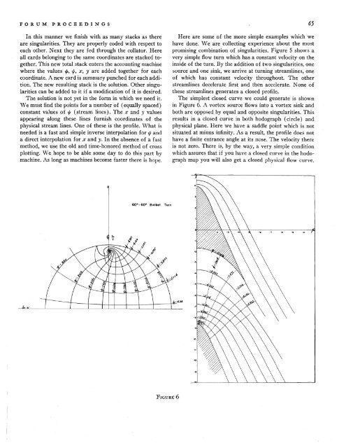
60· - 60· Bucket Turn
FIGURE 6
Here are some of the more simple examples which we
have done. We are collecting experience about the most
promising combination of singularities. Figure 5 shows· a
very simple flow turn which has a constant velocity on the
inside of the turn. By the addition of two singularities, one
source and one sink, we arrive at turning streamlines, one
of which has constant velocity throughout. The other
streamlines decelerate first and then accelerate. None of
these streamlines generates a closed profile.
The simplest closed curve we could generate is shown
in Figure 6. A vortex source flows into a vortex sink and
both are 0pP9sed by equal and opposite singularities. This
results in a closed curve in both hodograph (circle) and
physical plane. Here we have a saddle point which is not
situated at minus infinity. As a result, the profile does not
have a finite entrance angle at its nose. The velocity there
is not zero. There is, by the way, a very simple condition
which assures that if you have a closed curve in the hodograph
map you will also get a closed physical flow curve.
65