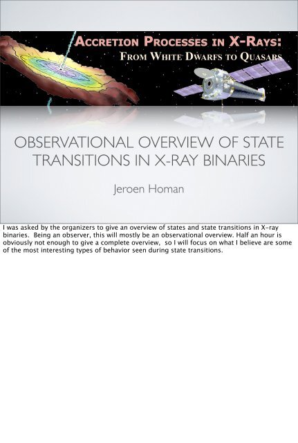
observational overview of state transitions in x-ray binaries

!""#$%&'()*#'"$++$+)&(),-#!.+/ 

4566789( :;6?@76A6B7@( CD5; 

9B>8BE7F(9C7(@95F=(>G(8(B8(FBA76@7(IC=@BH

BACKGROUND 

• Known since the 1970’s that X-ray binaries can show different 

spectral states (Cyg X-1, Tananbaum et al. 1972). 

• Reflect different modes of accretion (inflow/outflow) 

• mid 1980‘s - early 1990’s: EXOSAT and GINGA. Additional 

states identified in black hole binaries. Z and atoll classification 

for neutron star binaries. 

• State dependency of rapid X-ray variability and radio emission 

Let me first start with a little background. Observations of the black hole X-ray binary Cyg 

X-1 in the early 70’s showed that it displayed two distinct spectral states; a high luminosity 

state with a soft, thermal X-ray spectrum without radio emission, and a low-luminosity state 

with a hard, non-thermal spectrum accompanied with radio emission. The spectral states are 

now thought to reflect different modes of accretion onto a compact object. 

Observations between the mid 80s and early 90‘s with EXOSAT and Ginga revealed additional 

spectral states in black hole X-ray binaires and also distinct spectral states in neutron star 

sources (with the identification of the so-called Z and atoll sources). We also saw the first 

indications for a spectral state dependency of the rapid X-ray variability and radio emission. 

For the rest of the talk I will simply refer to spectral states as states, since it is not only the 

spectral properties that change.

MORE 

BACKGROUND 

• 1996>: Dedicated monitoring programs with Rossi X-ray 

Timing Explorer. Major progress. 

• SAX/Chandra/XMM/Suzaku/INTEGRAL are completing the 

X-ray picture. 

• Radio and nIR monitoring greatly expanded. Studies of jets. 

• Links with AGN / ULX 

Major progress in our understanding of states was made after the launch of the Rossi X-ray 

Timing Explorer, which performed many dedicated monitoring campaigns of transient and 

highly variably sources. This was important to establish the relation between the various 

states. 

It also provided a strong framework for observations with satellites that provide information 

that cannot be obtained with RXTE, most notably high resolution spectra to study winds and 

outflows, low energy coverage to study disk evolution, broader energy range, and highenergy 

coverage. 

The last decade has also seen an large increase in radio and nIR observations that allow 

studies of jet outflows. Together these observations are completing our picture of states and 

state transitions, at least in an observational sense, and allows for a better interpretation of 

the underlying changes in the accretion flow. 

Although I will not discuss the topic in my talk, observations of states in black hole X-ray 

binaries are also relavant to the study of AGN, as we heard earlier today, and also that of 

ULXs.

• black hole transients 

• light curves, hardness-intensity diagrams (HID) 

• implications for accretion flows 

• black hole states (classification) 

• variability (quasi-periodic oscillations - QPOs) 

• jets, winds - relation to states 

• neutron star transients 

OUTLINE 

Here’s a brief outline of the talk. Most of my talk will deal with black hole systems, as our 

knowledge of the different states appears to be a bit more complete. I’ll start with an 

overview of transient outbursts and will introduce the hardness-intensity diagram, which is 

useful tool to study the spectral evolution of transients. I’ll discuss some of the implications 

of the observed evolution for accretion flows. I’ll go on to identify the various states in the 

HID and summarize their spectral and variability properties. 

I’ll continue by showing how the different types of variability map onto the hardness intensity 

diagram. I will do the same for jets and winds. 

I’ll end with a brief comparison with neutron stars, where a lot of progress has been made 

recently.

TRANSIENT SOURCES 

• Relation between different states is best studied in transient 

(or highly variable) sources: 

• large change in mass accretion rate 

• Monitoring with RXTE has been very valuable 

For my discussion of states I'll limit myself to transient sources. These 

sources undergo large changes in the mass accretion rates during their 

outbursts, as the result of which they makes transitions between several 

states. 

Almost all observations that I will present today are from RXTE, which 

has been able to monitor the outbursts of tens of transients in great 

detail. Moreover, it gives two of the key ingredients necessary for 

classifying observations: broadband spectra and rapid variability

LONG-TERM LIGHT CURVES 

4U 1543-47 

GRO J1655-40 

RXTE All-Sky Monitor 

H1743-332 

GX 339-4 

Here I show a few examples of long-term light curves from the All-Sky monitor on RXTE. As 

you can see there is quite a variety in the duty cycle of these systems and also in the length 

and brightness of the outbursts of individual sources. The general consensus is the longterm 

transient behavior is the result of instabilities in the outer disk, just as in dwarf novae.

OUTBURST LIGHT CURVES 

4U 1543-47 

GRO J1655-40 

RXTE/PCA 

GX 339-4 

H1743-322 

Here I show a few examples of individual outbursts as observed with the RXTE/PCA. The large 

variety in outburst shapes is obvious. Outbursts typically last from a few weeks to a year. 

Some show a very fast rise to their peak, while in other sources it is much slower. Others 

show multiple peaks or very irregular shapes. Strong flaring, like shown here in GRO 

J1655-40 and H1743-322, is typically only seen in the brightest outbursts, which go above, 

say 20% Eddington.

LIGHT CURVE 

GX 339-4 

Let me illustrate the typical spectral evolution that is seen in most transient outburst. I’m 

taking GX 339-4 as an example, as it show fairly clean behavior, compared to some other 

systems. This is a light curve in the full RXTE/PCA energy band

ENERGY DEPENDENCE 

This movie (Homan_GX339-4_movie.mov) shows how the outburst shape depends on energy. 

During the movie the energy of the light curve goes down from 20 keV to 2 keV. In the high 

energy band we see a large peak at the start of the outburst. Going down to lower energies 

that peak disappears. Instead we see peaks appear later in the 

outburst. Obviously, there are considerable spectral changes during the outburst.

SPECTRAL EVOLUTION 

GX 339-4 

Let me go back to the full band light curve again and discuss in more 

detail the spectral (or color) evolution during an outburst


GX 339-4 

First I’ll switch to a logarithmic scale for the outburst, since some spectral evolution takes 

place at the lowest count rates. This way it is more convenient to get a look at changes at all 

luminosity levels

COLOR EVOLUTION 

hard soft 

hardest = power-law cominated (index 1.5) 

softest = accretion disk dominated (1 keV) 

GX 339-4 

hard 

hardness = 10.0-20.0 keV / 3.0-5.0 keV 

The next panel I’m adding shows the evolution of the spectral hardness, which is a simple 

ratio of count rates in two energy bands, in this case the 10-20 keV and 3.0/5.0 keV. It 

shows that the outburst starts with the source having a hard spectrum, switching to a soft 

spectrum, and at the end back to a hard spectrum. In this case the hardest spectra 

correspond to power-law dominated spectra, with an index of around 1.5, while the softest 

ones are accretion disk dominated, with a typical temperature of 1 keV. Note that the 

behavior seen in other black hole transients is mostly consistent with this, i.e. going from 

hard to soft and back to hard. By combining these two curves into a hardness-intensity 

diagram, we can see how this spectral evolution occurs as a function of the overall intensity 

level.

COLOR EVOLUTION 

hardness-intensity diagram (HID) 

Here is the HID that is the result of combining the light and hardness curves I just showed. 

The HID is a diagnostic plot 

that is used extensively in interpreting the X-ray evolution of black hole and neutron star Xray 

binaries. 

As a function of time, GX 339-4 traces out a q-shaped track during its bright outbursts. The 

branches that are shown correspond to different spectral states or transitions between them.


hardness-intensity diagram (HID) 

The arrows indicate the evolution in time. The source starts out faint and hard and increases 

in luminosity while the spectrum remains hard. At some point a sudden softening of the 

spectrum takes place, with only minor changes in the count rate. The spectrum remains soft 

as the source decays, but at some point the spectrum shows a sudden hardening and returns 

to the same hardness as at the start of the outburst. For the remainder of the decay the 

spectrum remains hard. The q-shaped diagram is traced out in an anti-clockwise manner. 

There are two important aspect of this diagram that should be noted. 

First, while at low luminosities the spectrum is always hard, at higher luminosities, the 

spectrum can be hard, soft, or of intermediate hardness. 

Second, the transition from hard to soft takes place at a significantly higher luminosity than 

the reverse transition. 

Similar behavior is also seen in other sources, as I will show later.

Luminosity (erg/s) 


ux 

hardness 

1- 

Disk Fraction 

Dunn et al. 2010 

Alternative ways to trace the evolution that actually involve some spectral fitting, produce 

similar looking diagrams. Here I’m showing a figure taken from a paper by Dunn et al. It 

show a so-called disk-fraction-luminosity diagram, where disk fraction is defined as the ratio 

of disk flux and total flux. It is useful to compare outbursts of different sources, but it 

requires a lot more work and is less sensitive to subtle changes. For comparison they show 

how certain selected observations in a HID map onto such a diagram - it clearly show the 

limitation to constrain disk fraction with RXTE, which is the reason I prefer to stick with the 

HID.

XTE J1752-223 

XTE J1908+094 


XTE J1650-500 

XTE J1550-564 

Here are four outburst from other sources. In three of them the rise of the outburst was not 

fully covered, but the behavior is consistent with what we saw in GX 339-4.

XTE J1752-223 

XTE J1908+094 


XTE J1650-500 

XTE J1550-564 

Again, q-shaped diagrams are traced out in and anti-clockwise manner. Note that this anticlockwise 

behavior is seen in almost all transients. The five HIDs I’ve showed so far are all 

from outburst in which no flaring was present. Let’s take a look at an outburst that does 

show flaring, since it shows some additional behavior.


GRO J1655-40 

Here is a light curve of GRO J1655-40, which shows clear flaring, with large changes in the 

count rate on a time scale of a day.


GRO J1655-40 

I’ll switch to a log scale again, which makes the flaring it little less impressive, but reveals 

more detail at low count rates.


hard 

GRO J1655-40 

And here I’m adding the hardness evolution. We still see the main hard -> soft -> hard 

transitions, but the behavior around the time of the flaring actually shows some changes in 

hardness as well. Let’s see what the HID looks like. 

soft 

hard


GRO J1655-40 

We still see a roughly q-shaped diagram, but on top of it we see some additional structure 

that corresponds to the flaring, and as I will show in a few minutes, this additional branch 

corresponds to a distinct spectral state.


GRO J1655-40 H1743-322 

XTE J1859+226 

brighter outburst: additional structure 

Here I show additional HIDs, which also show additional back and forth motion at their 

highest count rates, again corresponding to flaring in the light curve.


GX 339-4 

Transitions at 

different 

luminosities 

XTE 1550-564 

Not always full 

transitions 

Flaring only at 

high luminosity 

GRO J1655-40 

Flaring at similar 

luminosity 

The HIDs I showed until now were all from single outbursts. To complicate matters a bit, I’m 

going to show HIDs with multiple outbursts of the same source. First is GX 339-4, which 

clearly shows that transitions between states do not always occur at the same luminosity. 

In the second panel I show XTE J1550-564. The first outburst, in black, actually consistent of 

two parts, resulting in a complicated track. The red curve shows a different outburst, and it 

shows that transitions do not always make it to the soft side. In fact, in later outbursts this 

source never left the right branch of the HID. Also worth mentioning is the fact that the lower 

luminosity outburst did not show flaring. 

Finally two outbursts of GRO J16550. Unfortunately the red one was not covered in great 

detail, but at least it suggests that the additional structure due to the flaring falls in more or 

less the same location of the HID, suggesting that the ‘flaring branch’ has a more fixed 

relation to luminosity than the other branches with intermediate colors.


Yu & Yan 2009 

Some recent papers by Wenfei Yu and collaborators shed some new light on why these 

different paths can be traced out. They find that the luminosity at which the transitions from 

hard to soft take place correlates very well with the peak luminosity of the soft state that 

follows the transition. So somehow, at the time of the transition, the system already seems to 

have a knowledge of the maximum mass accretion rate that is going to be reached later on. 

Also, they find that the faster the rise of the transient, the higher the luminosity of the 

transition, which suggests that the path of a transient depends on the recent accretion rate 

history.

IMPLICATIONS FOR 

ACCRETION 

• outbursts must be driven by accretion rate changes 

• assuming count rate is roughly proportional to accretion rate: 

• no unique relation between accretion rate and spectral state 

• different paths for single sources suggest dependence on recent 

accretion history 

• ‘second paramater’ needed? 

• similar tracks seen for neutron stars, white dwarfs and AGN 

Before discussing the different branches in more detail, let me first note that some lessons 

about accretion flows can be learned from these simply diagrams. 

From spectral fits we know that the count rate in these diagrams is a reasonable tracer of the 

luminosity. We don’t know exactly how well it traces the accretion rate, but if we assume that 

it does so on a global scale, we most conclude that there is no one-to-one relation between 

the spectral state of the accretion flow and the mass accretion rate. This has led to the 

suggestion that there is a second independent parameter that determines the spectra state of 

a system, although I must say, I don’t really like that idea anymore. Moreover, the fact that 

even for a single source the evolution of and transitions between spectral states can change, 

strongly suggests that the recent accretion history plays an important role in determining the 

spectral state. 

These two properties appear to be a fundamental property of accretion flows, since we also 

see it in neutron star systems, dwarf novae, and AGN. However, it is not clear what is causing 

this behavior.

HYSTERESIS 

• Disc magnetization (Petrucci et al. 2008) 

• Compton cooling/heating (Liu et al. 2005) 

• Two flow model - Keplerian/sub-Keplarian (Chakrabarti and 

Titarchuk 1995, Smith et al. 2002) 

radial inflow 

standard accretion disk 

black 

hole 

•Accretion disk ‘feeds’ faster radial inflow 

•Could explain some of the behavior 

Some explanations have been proposed for the observed hysteresis. Pertucci et al. try to 

explain the hysteresis in terms of a large scale magnetic field that results in different 

luminosities for transitions between standard disk and jet producing disc. Liu et al. suggest 

that differences in Compton heating and cooling rates of the corona can explain the 

hysteresis. And finally, there is the two-flow accretion model which has been proposed by 

several authors, which I find a rather elegant solution, although I don’t have time to discuss it 

in detail.

STATE CLASSIFICATION 

• Various classification schemes, using (broadband) spectral and 

variability information 

• McClintock & Remillard 2005 (focused on three ‘stable’ 

states) 

• Homan & Belloni 2005 (focused on transitions) 

• Future schemes may use X-ray line spectra, multi-wavelength 

information, etc. 

Okay, let’s move on to the states. As I said before, states are typically defined as distinct 

combinations of X-ray spectral and variability properties, and, as I said earlier we believe that 

these states reflect different modes of accretion. 

Through the years various state classification schemes have been proposed, but the two most 

commonly used ones are the ones by McClintock and Remillard, which put more emphasis on 

the ‘stable’ states, and the one by myself and Tomaso Belloni, which puts more emphasis on 

the transitions between states. To a large extend these schemes are consistent though, and I 

will use definitions from both schemes 

With the wealth of multi-wavelength data becoming available, future schemes might actually 

include more than X-ray spectra and variability alone.

Relation between HID 

branches and states 

MAPPING THE STATES 

In the next few slides, I’ll summarize the properties of the various states and show how they 

map on to this hardness-intensity diagram of GRO J1655-40. 

Before I continue, first a few words on rapid X-ray variability, since together with X-ray 

spectra, it is a crucial ingredient of state classifications.

RAPID X-RAY VARIABILITY 

• power density spectra (1 mHz - 1 kHz) 

• broad (noise) and narrow (QPO) components 

• correlates with spectral properties and map well 

onto HID 

When I talk about rapid variability, I typically mean frequencies between 1 mHz and 1 kHz. 

This rapid variability is often studied terms in terms of power spectra, since most of the 

variability is too fast and/or too weak to be seen directly in the light curve. As Phil Uttley 

showed this morning, the power spectra often show combinations of broad components, 

which are often referred to as noise, and narrow features referred to as quasi-periodic 

oscillations, or QPOs. The rapid X-ray variability changes strongly between states and their 

evolution maps well onto the HID.

(McClintock & Remillard 2005) 

HARD STATE 

I’ll use the Figures from MClintock and Remillard to illustrate the spectral and variability 

properties, with energy spectra on the left and power spectra on the right. 

The first state that I show is the hard state, the most common state. This state has a very hard 

spectrum that is often completely dominated by a non-thermal component, whose origin is 

still a topic of debate, but is likely related to the presence of a steady radio jet outflow. The 

thermal accretion disk component is very weak in this state. 

Variability is very strong. The power spectra show very strong noise with corresponding 

amplitudes of 40%. QPOs are only seen when the source is becoming luminous and is close to 

a state transition. 

Hard states have been observed up to 20% Ledd, so the term low/hard that was often used is 

a bit of a misnomer. It is (together with the quiescent state) the only state observed below 1% 

Ledd. 

As mentioned before, sources in the hard state also show strong radio emission, with a flat or 

inverted spectrum, which indicates a self-absorbed compact jet. The jet also contributes 

significantly to the near-infrared emission.

• low-luminosity version of the 

hard state 

• slightly softer, still highly 

variable (V404 Cyg) 

• jet still present (falls on LX-LR 

relation - Gallo et al. 2006) 

QUIESCENCE 

The next state is quiescence. It is not really clear whether it is a separate state, or simply a 

low-luminosity version of the hard state. Quiescence is slight softer than quiescence, but 

appears still to be quite variable. Jets are still present at 10e-8 Ledd, following the same 

radio/X-ray relations seen in the hard state.

SOFT STATE 

The next state is called the soft state or the thermal dominant state. As the name already 

suggests, the spectrum is very soft and it is dominated by the thermal emission from the 

accretion disk - it is probably the best understood state. Weak non-thermal emission is also 

present in the form a weak tail. It’s origin is not well understood. Variability is very weak, 

with amplitudes of only a few percent of the total flux. QPO can be seen together if one 

combines data from many observations. Unlike the hard state, the soft state is only observed 

at high luminosities. 

There is no significant radio emission from the central source in the soft state.

INTERMEDIATE STATE 

Intermediate (transitional) states 

(TRANSITIONS) 

Moving on to the so-called intermediate states or transitional states. These correspond to the 

horizontal branches in the diagram. There is some debated as to whether these should be 

considered real states, or merely short lived unstable configurations. In the intermediate state 

the spectrum can be described by a combination of thermal and non-thermal emission, with 

the latter being stronger on the right hand side in the diagram. Not only the ratio of the two 

components changes, but also the slope of the non-thermal component, which steepens 

considerably. Both effects result in lower values of the hardness. 

Variability is interesting in this states. QPOs of different types are seen and I will describe 

their behavior shortly. Amplitudes decrease from tens of percent to a few percents. The 

intermediate state also gives radio to occasional radio flares. Radio emission usually starts to 

weaken when the source turns this corner, followed days later by a giant radio flare, 

associated with the ejection of matter in the form of an outflow. 

Intermediate states can be observed over a wide range of luminosities - typically the same as 

that of the soft state.

STEEP POWER-LAW STATE 

radio ejections 

Finally there’s the steep power-law state. In light curve this state is characterized by very 

strong flaring on a time scale of days. This state is only observed at the very highest 

luminosities. The spectrum of this state is dominated by a steep power -law component on 

top of a very hot accretion disk component. Again, the non-thermal component is poorly 

understood, but is is probably the results of inverse Compton scattering. 

We see many different types of power spectra and they seem to combine elements of power 

spectra seen in the other states, with different types of noise and QPOs. In the radio with 

often see optically thin ejection events. 

In a way it is quite similar to the intermediate state, with a hotter disk and the power-law 

changing in normalization rather than index. It has been suggested that this state 

corresponds to the presence of a thickened or slim disk.


Okay, let’s go back to see how the rapid X-ray variability evolves in the HID. First let me show 

how the overall strength of the variability changes.


0.1-100 Hz 

rms-drop 

Here I add an extra panel showing the integrated rms variability between 0.1 and 100 Hz. As 

one can see, the strength of the variability changes rather smoothly from a few tens of 

percent in the hard state down to a few percent in the soft state. Both in the hard state and in 

the soft state the power spectra are rather featureless, with broad components dominating 

the power spectra. Most of the interesting stuff occurs in between these two states, and this 

is also where we see a rather mysterious drop in the rms variability, as pointed out here. This 

drop in rms is related to a short and sudden changes in the power spectral properties, as I 

will show in the next slide.

Power 

type-B frequency up 

1 10 100 1000 

Power 

2 

2 5 10 20 50 100 

Frequency (Hz) 

0.01 0.1 1 10 100 1000 



Power 

1 10 100 1000 

rms-drop 

0.01 0.1 1 10 100 1000 


type-C frequency up 

Power 

1 10 100 1000 

0.01 0.1 1 10 100 1000 


hard 

Power 

1 10 100 1000 

0.01 0.1 1 10 100 1000 


Power 

1 10 100 1000 

0.01 0.1 1 10 100 1000 


High Frequency QPOs 

Let’s take a look at what happens during the transitions between the hard and soft state. 

These transitions are host to various types of QPOs, with the two most common ones being 

named type-B and type-C QPOs - not very imaginative. Let me start with the type-C. It 

usually sits on top of a strong noise component in a power spectrum. And it actually evolves 

from one of the broad noise components seen in the hard state. The evolution of the type-C 

power spectra is shown at the top. From hard to soft, or right to left, the type-C QPO 

increases in frequency by about a factor of a hundred, while it becomes weaker. Weak 

remnants of this QPO can be found in the soft state, and we found that the maximum 

frequency observed scales inversely with the mass of the black hole in the few systems in 

which it was found. The type-C QPOs can change from 0.01 to a few tens of Hz at varying 

luminosity levels. 

It is still not clear what the changes mean, but if the QPO frequency is related to a radius, for 

example the inner disk radius or the outer radius of the corona, this radius is getting smaller. 

Of course, as Phil mentioned earlier, it doesn’t have to be a radius, it could also be scale 

height of the disk for example. 

This smooth evolution in type-C QPOs is almost always briefly interrupted by a short and 

sudden change in the variability properties. At a more or less fixed value of the spectral 

hardness, we see a drop in the overall strength of the variability. Just before that we actually 

see a change in the type of QPO from type-C to type-B. The broad peaked noise component 

disappears as well. The evolution of type-B QPO, which is shown on the left, is actually quite 

different - rather than a frequency dependence on hardness, we see a dependence of 

frequency on luminosity. 

The zone of strange power spectral properties also gives rise to the so-called high frequency 

QPOs, wich are typically observed at a few hundred Hz. They are observed as single peaks, or 

as pairs. The single peaks can move around by up to 15-20%, but the pairs are only observed 

at fixed frequencies, sometimes even years apart, suggesting they are set by GR.

JETS 

radio and nIR monitoring: lots of progress 

We can try to do the same for jets. How does jet activity map onto the HID? The last decade 

has seen an enormous increase in the amount of radio and near-infrared observations, both 

of which can be used to study the evolution of jet outflows.

No Compact Jet 

(interaction with 

ISM) 

Fender, Belloni, Gallo 2004 

Fender, Homan, Belloni, 2009 


Ejection 

Events 

rms-drop 

type-B QPOs 

JETS 

Compact 

Jet Switches on 

(radio) 

Radio 

Flare 

hard 

Compact 

Jet Weakens 

(radio/nIR) 

Compact 

Jet 

Compact 

Jet Switches on 

(nIR) 

Homan et al. 2005 

Russell et al. 2006 

Coriat et al. 2009 

I’m going to use the same schematic again and will summarize the picture that is emerging 

from various radio and nIR papers. I’ll start with the hard state and progress through the 

diagram in an anti-clockwise manner. The hard state gives rise to steady radio emission from 

a compact jet. Radio and nIR emission scale in similar ways with the X-ray luminosity. Once a 

system turns the corner the radio and nIR start to weaken, suggesting the jet is getting less 

powerful. Than at some point during the transition a radio flare is observed, which is thought 

to be the result of an ejection event. Interestingly, this flare always seems to take place within 

a few days of this zone with odd variability properties that I just discussed. In sources that 

cross this zone multple times during an outburst, like XTE J1858+226, we see radio flares 

associated with rms drops in all cases. Bright sources that enter the steep power law state 

suggest that ejection events continue to occur in that state. 

No radio emission from the central source is seen in the soft state. If there is radio emission it 

is likely the result of interaction of the jet ejecta with the ISM. 

At some point the source starts it return to the hard state. We’re not exactly sure when the 

jet switches on again in the radio, but from at least one source it is clear that it start 

somewhere halfway in the transition, and perhaps even earlier. In the near-infrared jet 

emission only becomes significant when it reaches the hard state.

4 

H1743-322 

3 

1 

2 

WINDS 

Miller et al. 2006 

Of course, we can do the same as well for winds. In this case we rely on high resolution 

spectra to observe the line features from the wind, but unfortunately such simultaneous 

observations with RXTE are not very common. Nevertheless, I’ll decided to give it a try for two 

sources. 

First is an example from H1743-332. Four Chandra observations were made. Remember that 

radio emission is mostly confined to the right half of the track. The hardest of the four 

observations, nr 2, shows no absorption lines. The three softer ones do and indicate the 

presence of a wind outflow.

GRO J1655-40 

weak abs. lines 

weak emission lines 

WINDS 

keV -1 

) 

Residuals (Counts s -1 

5 

0 

-5 

-10 

-15 

-20 

-25 

-30 

5 6 7 8 9 10 

Energy (keV) 

The second example is GRO J1655-40, which had a few more observations. The hardest 

observation showed an iron emission lines (not shown on slide). Going to the softer ones, we 

start seeing weak absorption lines (not shown slide). The slightly harder observations, in 

green, start showing stronger iron absorption lines, and the softest one, marked by the red 

star, shows a complete forest of lines. This indicates an ever stronger growing wind as we 

move from hard to soft. This hints at an anti-correlation between jet outflows and wind 

outflows. Such an anti-correlation was more directly observed in the microquasar GRS 

1915+105 by Joey Neilsen and Julia 

Lee. Obviously, more simultaneous observations are needed to from a more complete picture.

NEUTRON STARS 

Two topics: 

•HID of ‘ordinary’ transients 

•HID evolution near LEdd 

In the last few slides I’d like to show some of the behavior seen in neutron star transients. I’ll 

discuss the HIDs of ordinary sub-Eddington transients as well as the evolution of our only 

super-Eddington transient.

Aql X-1 

NEUTRON STARS 

hard - soft - transitions 


transitional 

hard 

q-shaped 

anti-clockwise 

motion 

This is Aql X-1, a transient that shows frequency outbursts. The HID is q-shaped, like in black 

holes, and motion is anti-clockwise. The spectral evolution has very little to do with nature of 

compact object and as I mentioned earlier similar looking diagrams can be constructed for 

white dwarfs and AGN. Spectrally, the states in systems like this are very similar to black 

holes, except for an additional of a thermal component from the neutron star surface or 

boundary layer. Similar tracks are seen for almost all sub-Eddington transients. (below 20% 

Eddington)

NEUTRON STARS 

Jet Formation 

Aql X-1 

Miller-Jones et al. 2010 

A quick look at how radio maps onto the HID of sub-Eddington neutron star systems. The 

best example so far comes from Aql X-1. Overall behavior is quite similar to that of black 

holes.

Aql X-1 

Back to the HID again. 

NEUTRON STARS 



transitional 

hard 

q-shaped 

anti-clockwise 

motion

NEUTRON STARS 


hard 

transitional 


Let me flip the diagram around and increase the time resolution a bit, for my discussion of 

the super-Eddington transient XTE J1701-462. The same three states are identified in this 

diagram.

hard 

transitional 

Lin et al. 2009 



NEUTRON STARS 

XTE J1701-462: super-Eddington transient 

hard 

transitional 


I’ll make it a little smaller and add the HID of XTE J1701-462, starting with the lowluminosity 

phase. Unfortunately XTE J1701-462 moved very rapidly through its low 

luminosity phase, but we can still identify a hard, transitional and soft state.

hard 

transitional 




NEUTRON STARS 


hard 

transitional 


Moving up in luminosity we start seeing some flaring, perhaps similar to that seen in BHCs.



NEUTRON STARS 


Flaring becomes stronger at higher luminosities (i.e. more pronounced in count rate).



NEUTRON STARS 


Z source (Sco X-1 like) 

At some point we start seeing an additional branch and the source is actually turning into a Z 

source, similar to Sco X-1.



NEUTRON STARS 


Z source (Sco X-1 like) 

At higher luminosity a more complete Sco-like Z track can be seen.



NEUTRON STARS 


Z source (Cyg X-2 like) 

And at even higher luminosities we see Z source behavior similar to Cyg X-2.



NEUTRON STARS 


Z source (Cyg X-2 like) 

And finally, at the highest luminosities the source start to become a little crazy, with 

enormous luminosity swings. 

This completes for the first time our view of behavior from super-Eddington to lower Lx, 

something we still don’t have in BHCs unfortunately.

CONCLUSIONS 

• HIDs provide quick overview of spectral evolution and reveal 

complex behavior 

• Variability properties map well onto HID. Sudden change in 

timing related to HFQPOs and radio flares 

• Jet activity maps well onto HID - anti-correlated with winds? 

• Neutron stars show similar evolution. However, above 0.2 LEdd 

they become crazy 

• Slowly completing our picture of states, allowing for more 

detailed interpretation

observational overview of state transitions in x-ray binaries

Create successful ePaper yourself

Delete template?

Save as template?