This issue is sponsored by the Philips Romania, Lighting Division
This issue is sponsored by the Philips Romania, Lighting Division
This issue is sponsored by the Philips Romania, Lighting Division
Create successful ePaper yourself
Turn your PDF publications into a flip-book with our unique Google optimized e-Paper software.
C Ţicleanu<br />
and vector of parameters a of arbitrary<br />
length. Note that using <strong>the</strong> LM method,<br />
any nonlinear equation with an arbitrary<br />
number of parameters can be used as <strong>the</strong><br />
data modelling equation. Then, <strong>the</strong> “merit<br />
function” we are trying to minimize <strong>is</strong><br />
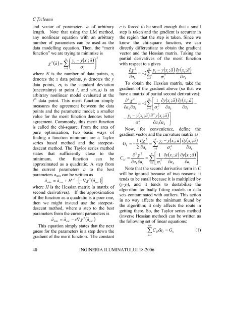
N<br />
r 2<br />
2 r ⎛ yi<br />
− y(<br />
xi<br />
; a)<br />
⎞<br />
χ ( a)<br />
= ∑ ⎜<br />
⎟<br />
i= 1 ⎝ σ i ⎠<br />
where N <strong>is</strong> <strong>the</strong> number of data points, xi<br />
denotes <strong>the</strong> x data points, yi denotes <strong>the</strong> y<br />
data points, σi <strong>is</strong> <strong>the</strong> standard deviation<br />
(uncertainty) at point i, and y(xi,a) <strong>is</strong> an<br />
arbitrary nonlinear model evaluated at <strong>the</strong><br />
i th data point. <strong>Th<strong>is</strong></strong> merit function simply<br />
measures <strong>the</strong> agreement between <strong>the</strong> data<br />
points and <strong>the</strong> parametric model; a smaller<br />
value for <strong>the</strong> merit function denotes better<br />
agreement. Commonly, th<strong>is</strong> merit function<br />
<strong>is</strong> called <strong>the</strong> chi-square. From <strong>the</strong> area of<br />
pure optimization, two basic ways of<br />
finding a function minimum are a Taylor<br />
series based method and <strong>the</strong> steepestdescent<br />
method. The Taylor series method<br />
states that sufficiently close to <strong>the</strong><br />
minimum, <strong>the</strong> function can be<br />
approximated as a quadratic. A step from<br />
<strong>the</strong> current parameters a to <strong>the</strong> best<br />
parameters amin can be written as<br />
r r<br />
−1<br />
2 r<br />
amin<br />
= acur<br />
+ H ⋅ [ − ∇χ<br />
( acur<br />
) ]<br />
where H <strong>is</strong> <strong>the</strong> Hessian matrix (a matrix of<br />
second derivatives). If <strong>the</strong> approximation<br />
of <strong>the</strong> function as a quadratic <strong>is</strong> a poor one,<br />
<strong>the</strong>n we might instead use <strong>the</strong> steepestdescent<br />
method, where a step to <strong>the</strong> best<br />
parameters from <strong>the</strong> current parameters <strong>is</strong><br />
r r<br />
2 r<br />
amin<br />
= acur<br />
− c∇χ<br />
( acur<br />
)<br />
<strong>Th<strong>is</strong></strong> equation simply states that <strong>the</strong> next<br />
guess for <strong>the</strong> parameters <strong>is</strong> a step down <strong>the</strong><br />
gradient of <strong>the</strong> merit function. The constant<br />
40<br />
c <strong>is</strong> forced to be small enough that a small<br />
step <strong>is</strong> taken and <strong>the</strong> gradient <strong>is</strong> accurate in<br />
<strong>the</strong> region that <strong>the</strong> step <strong>is</strong> taken. Since we<br />
know <strong>the</strong> chi-square function, we can<br />
directly differentiate to obtain <strong>the</strong> gradient<br />
vector and <strong>the</strong> Hessian matrix. Taking <strong>the</strong><br />
partial derivatives of <strong>the</strong> merit function<br />
with respect to a gives<br />
2 N r r<br />
∂χ<br />
yi<br />
− y(<br />
xi<br />
; a)<br />
∂y(<br />
xi<br />
; a)<br />
= −2∑<br />
2<br />
∂ak<br />
i= 1 σ i ∂ak<br />
To obtain <strong>the</strong> Hessian matrix, take <strong>the</strong><br />
gradient of <strong>the</strong> gradient above (so that we<br />
have a matrix of partial second derivatives):<br />
2 2<br />
N<br />
r r<br />
∂ χ ⎡ 1 ∂y(<br />
xi<br />
; a)<br />
∂y(<br />
xi<br />
; a)<br />
= −2∑<br />
⎢<br />
−<br />
2<br />
∂ak<br />
∂al<br />
i= 1 ⎣σ<br />
i ∂ak<br />
∂al<br />
r 2 r<br />
y − ( ) ∂ ( ) ⎤<br />
i y xi<br />
; a y xi<br />
; a<br />
− 2<br />
⎥⎦<br />
σ ∂a<br />
∂a<br />
i<br />
l<br />
Now, for convenience, define <strong>the</strong><br />
gradient vector and <strong>the</strong> curvature matrix as<br />
2 N r r<br />
1 ∂χ<br />
yi<br />
− y(<br />
xi<br />
; a)<br />
∂y(<br />
xi<br />
; a)<br />
Gk<br />
= − = ∑ 2<br />
2 ∂ak<br />
i= 1 σ i ∂ak<br />
2 2 N<br />
r r<br />
∂ χ ⎡ 1 ∂y(<br />
x ) ∂ ( ) ⎤<br />
i ; a y xi<br />
; a<br />
Ckl<br />
= = ∑ ⎢ 2<br />
⎥<br />
∂ak<br />
∂al<br />
i= 1 ⎣σ<br />
i ∂ak<br />
∂al<br />
⎦<br />
Note that <strong>the</strong> second derivative term in C<br />
will be ignored because of two reasons: it<br />
tends to be small because it <strong>is</strong> multiplied <strong>by</strong><br />
(y-yi), and it tends to destabilize <strong>the</strong><br />
algorithm for badly fitting models or data<br />
sets contaminated with outliers. <strong>Th<strong>is</strong></strong> action<br />
in no way affects <strong>the</strong> minimum found <strong>by</strong><br />
<strong>the</strong> algorithm; it only affects <strong>the</strong> route in<br />
getting <strong>the</strong>re. So, <strong>the</strong> Taylor series method<br />
(inverse Hessian method) can be written as<br />
<strong>the</strong> following set of linear equations:<br />
NP<br />
∑<br />
k =1<br />
INGINERIA ILUMINATULUI 18-2006<br />
kl<br />
l<br />
k<br />
C δ a = G<br />
(1)<br />
k


