This issue is sponsored by the Philips Romania, Lighting Division
This issue is sponsored by the Philips Romania, Lighting Division
This issue is sponsored by the Philips Romania, Lighting Division
Create successful ePaper yourself
Turn your PDF publications into a flip-book with our unique Google optimized e-Paper software.
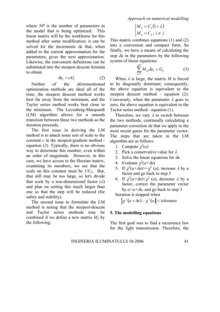
where NP <strong>is</strong> <strong>the</strong> number of parameters in<br />
<strong>the</strong> model that <strong>is</strong> being optimized. <strong>Th<strong>is</strong></strong><br />
linear matrix will be <strong>the</strong> workhorse for th<strong>is</strong><br />
method after some modification; it can be<br />
solved for <strong>the</strong> increments δa that, when<br />
added to <strong>the</strong> current approximation for <strong>the</strong><br />
parameters, gives <strong>the</strong> next approximation.<br />
Likew<strong>is</strong>e, <strong>the</strong> convenient definitions can be<br />
substituted into <strong>the</strong> steepest descent formula<br />
to obtain<br />
δ a l = cGl<br />
(2)<br />
Nei<strong>the</strong>r of <strong>the</strong> aforementioned<br />
optimization methods are ideal all of <strong>the</strong><br />
time; <strong>the</strong> steepest descent method works<br />
best far away from <strong>the</strong> minimum, and <strong>the</strong><br />
Taylor series method works best close to<br />
<strong>the</strong> minimum. The Levenberg-Marquardt<br />
(LM) algorithm allows for a smooth<br />
transition between <strong>the</strong>se two methods as <strong>the</strong><br />
iteration proceeds.<br />
The first <strong><strong>is</strong>sue</strong> in deriving <strong>the</strong> LM<br />
method <strong>is</strong> to attach some sort of scale to <strong>the</strong><br />
constant c in <strong>the</strong> steepest-gradient method -<br />
equation (2). Typically, <strong>the</strong>re <strong>is</strong> no obvious<br />
way to determine th<strong>is</strong> number, even within<br />
an order of magnitude. However, in th<strong>is</strong><br />
case, we have access to <strong>the</strong> Hessian matrix;<br />
examining its members, we see that <strong>the</strong><br />
scale on th<strong>is</strong> constant must be 1/Cll. But,<br />
that still may be too large, so let's divide<br />
that scale <strong>by</strong> a non-dimensional factor (λ)<br />
and plan on setting th<strong>is</strong> much larger than<br />
one so that <strong>the</strong> step will be reduced (for<br />
safety and stability).<br />
The second <strong><strong>is</strong>sue</strong> to formulate <strong>the</strong> LM<br />
method <strong>is</strong> noting that <strong>the</strong> steepest-descent<br />
and Taylor series methods may be<br />
combined if we define a new matrix Mij <strong>by</strong><br />
<strong>the</strong> following:<br />
Approach on numerical modelling<br />
( 1+ λ )<br />
⎧M<br />
ii = Cii<br />
⎨<br />
⎩M<br />
ij = Cij<br />
, i ≠ j<br />
<strong>Th<strong>is</strong></strong> matrix combines equations (1) and (2)<br />
into a convenient and compact form. So<br />
finally, we have a means of calculating <strong>the</strong><br />
step δa in <strong>the</strong> parameters <strong>by</strong> <strong>the</strong> following<br />
system of linear equations:<br />
NP<br />
∑<br />
k =1<br />
M δ a = G (3)<br />
kl<br />
When λ <strong>is</strong> large, <strong>the</strong> matrix M <strong>is</strong> forced<br />
to be diagonally dominant; consequently,<br />
<strong>the</strong> above equation <strong>is</strong> equivalent to <strong>the</strong><br />
steepest descent method - equation (2).<br />
Conversely, when <strong>the</strong> parameter λ goes to<br />
zero, <strong>the</strong> above equation <strong>is</strong> equivalent to <strong>the</strong><br />
Taylor series method - equation (1).<br />
Therefore, we vary λ to switch between<br />
<strong>the</strong> two methods, continually calculating a<br />
parameter correction δa that we apply to <strong>the</strong><br />
most recent guess for <strong>the</strong> parameter vector.<br />
The steps that are taken in <strong>the</strong> LM<br />
algorithm are as follows:<br />
1. Compute χ 2 (a)<br />
2. Pick a conservative value for λ<br />
3. Solve <strong>the</strong> linear equations for δa<br />
4. Evaluate χ 2 (a+δa)<br />
5. If χ 2 (a+δa)>=χ 2 (a), increase λ <strong>by</strong> a<br />
factor and go back to step 3<br />
6. If χ 2 (a+δa)


