Download PDF - Springer

More documents

Recommendations

Info

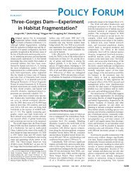
224 BERLING-WOLFF AND WU Figure 3. The land use maps of the Phoenix metropolitan area in 1975 and 1995: (A) empirical map of 1975 compiled from survey data, (B) empirical map of 1995 compiled from remote sensing and survey data, and (C) simulated map from PHX-UGM with a grain size of 120 m.
MODELING URBAN LANDSCAPE DYNAMICS 225 indicated that comparison at one single resolution was not adequate for evaluating spatial models and thus suggested a multiple-resolution measure, or a multi-scale goodnessof-fit. This method requires intensive resampling with a moving window whose size is increased progressively. The average goodness-of-fit is repetitively calculated at each window size. The formula for the fit at a particular sampling window size, Fw,is(Turner et al., 1989): Fw = P tw s=1 1 − tw i=1 [a1i −a2i ] 2w 2 s where w is the linear dimension of the (square) sampling window, aki (k = 1, 2; referring to the two maps to be compared) is the number of cells of category i in scene k in the sampling window, P is the number of different categories in the sampling window, s denotes the moving window that slides through the map one cell at a time, and tw is the total number of sampling windows in the map for window size w. Iftwo maps are identical, Fw = 1, and it remains 1 for all sampling window sizes (w); if two maps have the same proportions of cover types, but very different spatial pattern, Fw will increase gradually with the window size; if the spatial patterns of the two maps are slightly different, Fw will increase rapidly at first and soon start to approach 1 (Turner et al., 1989). We selected seven window sizes (1 × 1, 2 × 2, 4 × 4, 8 × 8, 16 × 16, 32 × 32, and 64 × 64 pixels), and a multi-scale goodness-of-fit plot was accordingly constructed (figure 4). In all cases, Fw increased rapidly first and then tended to approach the maximum value of 1 (figure 4a). While the overall goodness-of-fit was quite high for all window sizes (due partly to the large proportion of desert area), the mean value of Fw (averaged over all window sizes) varied among the five different grain sizes (figure 4b). To quantify the differences, we had 30 simulation runs at each grain size and then computed the mean goodness-of-fit over all sampling window sizes for each grain size. This result suggested the existence of a limited range of grain sizes (i.e., 120–480 meters) for which the overall fit of the model was higher. Landscape indices Error matrix and multiple resolution goodness-of-fit are valuable for assessing the accuracy of spatial models, but it is difficult to determine how well the spatial patterns of the modeled and empirical maps match each other. However, the model accuracy in terms of spatial patterns may be important ecologically and technically, and can be assessed using landscape indices (Turner et al., 1989). Landscape ecologists have developed and applied a suite of indices to quantify spatial patterns in the past two decades (O’Neill et al., 1988; Turner et al., 1991; Gustafson, 1998; Wu et al., 2002). We used FRAGSTATS, a landscape analysis package developed by McGarigal and Marks (1995), to compute the values of 18 selected metrics at different grain sizes (Wu et al., 2002; Wu, 2004). However, to reduce redundancy we report the results of only 6 metrics: number of patches (NP), edge density (ED), mean patch size (MPS), patch size coefficient of variation (2)
Page 1 and 2: Urban Ecosystems, 7: 215-240, 2004
Page 3 and 4: MODELING URBAN LANDSCAPE DYNAMICS 2
Page 9: MODELING URBAN LANDSCAPE DYNAMICS 2

Download PDF - Springer

Create successful ePaper yourself

Delete template?

Save as template?