Download PDF - Springer

228 BERLING-WOLFF AND WU
we desire to detect, γ is the degrees of freedom of the sample standard deviation with b
groups of samples and n samples per group (or γ = b(n − 1)), α is the significance level,
P is the desired probability that a difference will be found to be significant if it is as small
as δ and tα,γ and t2(1−P),γ are values from a two-tailed t-table with γ degrees of freedom
corresponding to probabilities of α and 2(1 − P), respectively. One cannot solve for n
directly because γ is a function of n. Instead, one guesses a value of n, calculates γ , then
solves the equation for n.Ifthe calculated n is not equal to the guessed n,adifferent value
of n is guessed accordingly and the procedure repeats. Here, an estimate of the variability
of selected sampling items (in this case landscape indices) needs to be obtained by running
30 baseline simulations and calculating the sample variance. The minimum number of runs
required to compute the mean of each of the 6 selected metrics is listed in Table 2. At
the landscape level, the minimum number of runs tended to increase with increasing grain
size (i.e., decreasing resolution), but such a trend was absent at the class level (Table 2).
Instead, the finest and coarsest grain sizes required the largest number of runs for deriving
meaningful means of the metrics. To simplify the simulation procedures, we derived the
means of all the metrics based on 30 simulation runs, which was larger than the minimum
number of runs for most landscape metrics (except NP and MPS) at all grain sizes based
on Eq. 3.
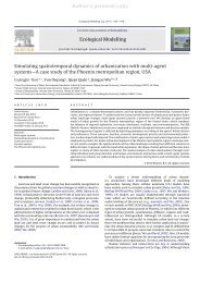
Figure 5 shows the results of the six landscape metrics computed for both the whole
landscape including all land use types and the urban class only. The relative differences
between the model and data at each grain size are listed in Table 3. In general, two kinds
of scale effects were apparent: (1) the values of the landscape metrics changed with grain
size (Wu, 2004), and (2) the agreement between the model and the empirical data also
varied with grain size. For a given metric, these scale effects showed similar patterns at
the urban class and the whole landscape levels, but model accuracy measured by these
metrics was consistently higher at the landscape level than the class level (Table 3). Specifically,
the values of the number of patches, edge density, and patch size coefficient of
variation decreased with grain size, and the discrepancy between the model and data measured
by these metrics was greatest at the 60 m grain size, smallest at the 120 m grain
size, and moderate to small for larger grain sizes (figures 5a–d, g–h; Table 3). The average
shape of individual patches (AWMSI) showed a similar pattern without the dramatically
large discrepancy at the finest grain size (figures 5i–j). In contrast, the mean size
of individual patches (MPS) and the shape complexity of the whole landscape (DLFD)
tended to increase with grain size, and so did the model errors represented by these metrics
(figures 5e–f, k–l).
Projecting future urban growth of Phoenix
A major goal of this study was to explore how the Phoenix urban landscape would change
in the future. To achieve this goal, we designed three development scenarios based on
the current political climate and the desires of the residents, and then ran simulations to
examine how these scenarios led to different future development patterns. The sources of
information for developing these scenarios include the Maricopa County Comprehensive