- Page 1:
Université Paris Diderot UFR de Ph
- Page 5 and 6:
Remerciements i Dans le cadre profe
- Page 7 and 8:
Table des matières Remerciements i
- Page 9 and 10:
Curriculum vitæ État civil Né le
- Page 11 and 12:
Activités d’encadrement Encadrem
- Page 13 and 14:
Résumé Résumé ix Mes travaux de
- Page 15 and 16:
Abstract Abstract xi The scientific
- Page 17:
EXPOSÉ DES RECHERCHES
- Page 20 and 21:
4 Introduction identifiées par leu
- Page 22 and 23:
6 Introduction - Le symbole Lv dés
- Page 25 and 26:
Une première étape pour la résol
- Page 27 and 28:
à chaque instant, et seules deux
- Page 29 and 30:
Chapitre 1 A constrained scheme for
- Page 31 and 32:
1.1 Introduction and motivations 15
- Page 33 and 34:
1.2 Covariant 3+1 conformal decompo
- Page 35 and 36:
1.2 Covariant 3+1 conformal decompo
- Page 37 and 38:
where 1.2 Covariant 3+1 conformal d
- Page 39 and 40:
1.3 Einstein equations in terms of
- Page 41 and 42:
1.3 Einstein equations in terms of
- Page 43 and 44:
1.4 Maximal slicing and Dirac gauge
- Page 45 and 46:
with ˜R ij ∗ = 1 2 1.4 Maximal
- Page 47 and 48:
1.4 Maximal slicing and Dirac gauge
- Page 49 and 50:
1.5 A resolution scheme based on sp
- Page 51 and 52:
1.5 A resolution scheme based on sp
- Page 53 and 54:
(e î ), 1.5 A resolution scheme ba
- Page 55 and 56:
1.5 A resolution scheme based on sp
- Page 57 and 58:
Asymptotic behavior 1.5 A resolutio
- Page 59 and 60:
1.5 A resolution scheme based on sp
- Page 61 and 62:
1.6 First results from a numerical
- Page 63 and 64:
Relative error on d Psi / dt 0.01 0
- Page 65 and 66:
1.A Degenerate elliptic operators o
- Page 67 and 68:
Chapitre 2 Mathematical issues in a
- Page 69 and 70:
2.1 A Fully-Constrained evolution s
- Page 71 and 72:
2.1 A Fully-Constrained evolution s
- Page 73 and 74:
2.2 First-order reduction of the re
- Page 75 and 76:
2.3 Characteristic structure of the
- Page 77 and 78:
2.3 Characteristic structure of the
- Page 79 and 80:
2.4 Dirac gauge and system of conse
- Page 81 and 82:
following six scalar fields: 2.5 Di
- Page 83 and 84:
2.6 Discussion. 67 Then the six sca
- Page 85 and 86:
Chapitre 3 Improved constrained sch
- Page 87 and 88:
3.2 The fully constrained formalism
- Page 89 and 90:
3.2 The fully constrained formalism
- Page 91 and 92:
3.3 The new scheme in the conformal
- Page 93 and 94:
3.3 The new scheme in the conformal
- Page 95 and 96:
3.4 Numerical results 79 where the
- Page 97 and 98:
3.4 Numerical results 81 of nd −
- Page 99 and 100:
N c 10 0 10 -1 10 -2 10 -3 D1 D4 SU
- Page 101 and 102:
3.5 Generalization to the fully con
- Page 103 and 104:
3.6 Discussion 87 which is equivale
- Page 105 and 106:
3.6 Discussion 89 used recently by
- Page 107 and 108:
3.A Consistency of the approximatio
- Page 109:
Deuxième partie Méthodes spectral
- Page 112 and 113:
96 les coalescences de binaires d
- Page 115 and 116:
Chapitre 4 Spectral methods for num
- Page 117 and 118:
4.1 Introduction 101 In a more form
- Page 119 and 120:
4.1 Introduction 103 with a similar
- Page 121 and 122:
4.2 Concepts in One Dimension 4.2 C
- Page 123 and 124:
y 4 3 2 1 0 -1 -2 4.2 Concepts in O
- Page 125 and 126:
y 1 0.5 0 -0.5 N=4 -1 -0.5 0 0.5 1
- Page 127 and 128:
• Gauss quadrature: δ = 1. • G
- Page 129 and 130:
4.2 Concepts in One Dimension 113 T
- Page 131 and 132:
0.5 -0.5 Chebyshev polynomials 1 0
- Page 133 and 134:
max Λ |I N f -f| 10 0 10 -3 10 -6
- Page 135 and 136:
4.2 Concepts in One Dimension 119 F
- Page 137 and 138:
0.5 0.4 0.3 0.2 0.1 N=4 Exact solut
- Page 139 and 140:
0.5 0.4 0.3 0.2 0.1 N=4 Exact solut
- Page 141 and 142:
4.2 Concepts in One Dimension 125 T
- Page 143 and 144:
domain): ξ ′ nu ′ dx = ξn (
- Page 145 and 146:
Error 10 -4 10 -8 10 -12 10 -16 4.2
- Page 147 and 148:
4.3 Multidimensional Cases 131 The
- Page 149 and 150:
4.3 Multidimensional Cases 133 matc
- Page 151 and 152:
4.3 Multidimensional Cases 135 the
- Page 153 and 154:
4.3 Multidimensional Cases 137 for
- Page 155 and 156:
4.3.3 Going further 4.3 Multidimens
- Page 157 and 158:
4.4 Time-Dependent Problems 4.4 Tim
- Page 159 and 160:
Stability 4.4 Time-Dependent Proble
- Page 161 and 162: Imaginary part 4.4 Time-Dependent P
- Page 163 and 164: Strong enforcement 4.4 Time-Depende
- Page 165 and 166: 4.4 Time-Dependent Problems 149 Thu
- Page 167 and 168: 4.4 Time-Dependent Problems 151 the
- Page 169 and 170: 4.4 Time-Dependent Problems 153 Bou
- Page 171 and 172: 4.4 Time-Dependent Problems 155 the
- Page 173 and 174: 4.4 Time-Dependent Problems 157 4.4
- Page 175 and 176: 4.5 Stationary Computations and Ini
- Page 177 and 178: 4.5 Stationary Computations and Ini
- Page 179 and 180: 4.5 Stationary Computations and Ini
- Page 181 and 182: 4.5 Stationary Computations and Ini
- Page 183 and 184: Extensions 4.5 Stationary Computati
- Page 185 and 186: 4.5 Stationary Computations and Ini
- Page 187 and 188: 4.5 Stationary Computations and Ini
- Page 189 and 190: 4.6 Dynamic Evolution of Relativist
- Page 191 and 192: 4.6 Dynamic Evolution of Relativist
- Page 193 and 194: 4.6 Dynamic Evolution of Relativist
- Page 195 and 196: 4.6 Dynamic Evolution of Relativist
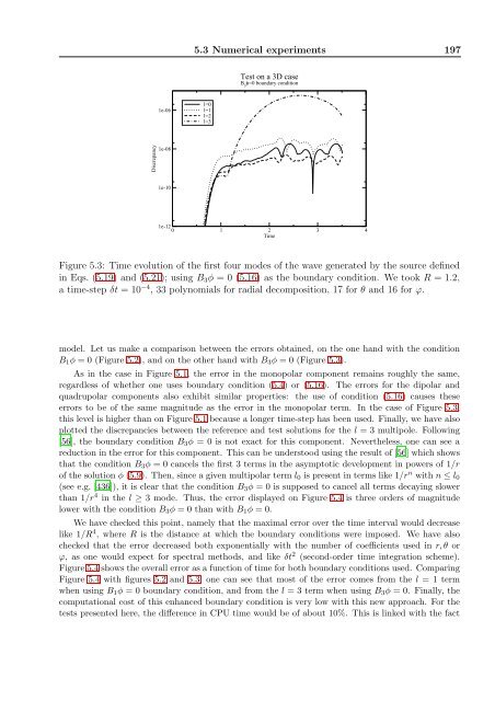
- Page 197 and 198: 4.6 Dynamic Evolution of Relativist
- Page 199 and 200: 4.6 Dynamic Evolution of Relativist
- Page 201 and 202: 4.6 Dynamic Evolution of Relativist
- Page 203 and 204: 4.7.3 Future developments 4.7 Concl
- Page 205 and 206: Chapitre 5 Absorbing boundary condi
- Page 207 and 208: 5.2 Absorbing boundary conditions 1
- Page 209 and 210: 5.2 Absorbing boundary conditions 1
- Page 211: Error on each multipolar component
- Page 215 and 216: 5.4 Conclusions 199 Our approach is
- Page 217 and 218: Chapitre 6 A spectral method for th
- Page 219 and 220: 6.1 Introduction 203 system we stud
- Page 221 and 222: defined from the scalar spherical h
- Page 223 and 224: 6.2 Vector case 207 6.2.3 Link with
- Page 225 and 226: 6.3 Symmetric tensor case 209 indic
- Page 227 and 228: 6.3.2 Divergence-free degrees of fr
- Page 229 and 230: 6.3.3 Traceless case 6.3 Symmetric
- Page 231 and 232: 6.4 Boundary conditions 215 There r
- Page 233 and 234: 6.4 Boundary conditions 217 When ex
- Page 235 and 236: Absolute error 0,01 0,0001 1e-06 1e
- Page 237 and 238: Absolute error 0.01 0.0001 1e-06 1e
- Page 239 and 240: 6.6 Concluding remarks 223 onto vec
- Page 241 and 242: Chapitre 7 A new spectral apparent
- Page 243 and 244: 7.3 The Nakamura et al. algorithm 2
- Page 245 and 246: We also expand all tensor fields on
- Page 247 and 248: 7.5 Tests 231 Table 7.1: Convergenc
- Page 249 and 250: 7.5 Tests 233 Table 7.2: Robustness
- Page 251 and 252: z 1.5 1 0.5 7.6 Conclusions 235 N
- Page 253: Troisième partie Simulations d’a
- Page 256 and 257: 240 mais requièrent beaucoup de m
- Page 258 and 259: 242 représente les neutrons superf
- Page 260 and 261: 244
- Page 262 and 263:
246 “Mariage des maillages” (Di
- Page 264 and 265:
248 “Mariage des maillages” (Di
- Page 266 and 267:
250 “Mariage des maillages” (Di
- Page 268 and 269:
252 “Mariage des maillages” (Di
- Page 270 and 271:
254 “Mariage des maillages” (Di
- Page 272 and 273:
256 “Mariage des maillages” (Di
- Page 274 and 275:
258 “Mariage des maillages” (Di
- Page 276 and 277:
260 “Mariage des maillages” (Di
- Page 278 and 279:
262 “Mariage des maillages” (Di
- Page 280 and 281:
264 “Mariage des maillages” (Di
- Page 282 and 283:
266 “Mariage des maillages” (Di
- Page 284 and 285:
268 “Mariage des maillages” (Di
- Page 286 and 287:
270 “Mariage des maillages” (Di
- Page 288 and 289:
272 “Mariage des maillages” (Di
- Page 290 and 291:
274 “Mariage des maillages” (Di
- Page 292 and 293:
276 “Mariage des maillages” (Di
- Page 294 and 295:
278 “Mariage des maillages” (Di
- Page 296 and 297:
280 “Mariage des maillages” (Di
- Page 298 and 299:
282 “Mariage des maillages” (Di
- Page 300 and 301:
284 “Mariage des maillages” (Di
- Page 302 and 303:
286 “Mariage des maillages” (Di
- Page 304 and 305:
288 “Mariage des maillages” (Di
- Page 306 and 307:
290 “Mariage des maillages” (Di
- Page 308 and 309:
292 “Mariage des maillages” (Di
- Page 310 and 311:
294 Rotating stars in Dirac gauge (
- Page 312 and 313:
296 Rotating stars in Dirac gauge (
- Page 314 and 315:
298 Rotating stars in Dirac gauge (
- Page 316 and 317:
300 Rotating stars in Dirac gauge (
- Page 318 and 319:
302 Rotating stars in Dirac gauge (
- Page 320 and 321:
304 Rotating stars in Dirac gauge (
- Page 322 and 323:
306 Rotating stars in Dirac gauge (
- Page 324 and 325:
308 Rotating stars in Dirac gauge (
- Page 326 and 327:
310 Rotating stars in Dirac gauge (
- Page 328 and 329:
312 Superluid neutron stars (Prix e
- Page 330 and 331:
314 Superluid neutron stars (Prix e
- Page 332 and 333:
316 Superluid neutron stars (Prix e
- Page 334 and 335:
318 Superluid neutron stars (Prix e
- Page 336 and 337:
320 Superluid neutron stars (Prix e
- Page 338 and 339:
322 Superluid neutron stars (Prix e
- Page 340 and 341:
324 Superluid neutron stars (Prix e
- Page 342 and 343:
326 Superluid neutron stars (Prix e
- Page 344 and 345:
328 Superluid neutron stars (Prix e
- Page 346 and 347:
330 Superluid neutron stars (Prix e
- Page 348 and 349:
332 Superluid neutron stars (Prix e
- Page 350 and 351:
334 Superluid neutron stars (Prix e
- Page 352 and 353:
336 Superluid neutron stars (Prix e
- Page 354 and 355:
338 Superluid neutron stars (Prix e
- Page 356 and 357:
340 Superluid neutron stars (Prix e
- Page 358 and 359:
342 Gyromagnetic ratio of relativis
- Page 360 and 361:
344 Gyromagnetic ratio of relativis
- Page 362 and 363:
346 Gyromagnetic ratio of relativis
- Page 364 and 365:
348 Gyromagnetic ratio of relativis
- Page 366 and 367:
350 Gyromagnetic ratio of relativis
- Page 368 and 369:
352 Gyromagnetic ratio of relativis
- Page 370 and 371:
354 Collapse of stable neutron star
- Page 372 and 373:
356 Collapse of stable neutron star
- Page 374 and 375:
358 Collapse of stable neutron star
- Page 376 and 377:
360 Collapse of stable neutron star
- Page 378 and 379:
362 Collapse of stable neutron star
- Page 380 and 381:
364 Collapse of stable neutron star
- Page 382 and 383:
366 Kerr solution in Dirac gauge (V
- Page 384 and 385:
368 Kerr solution in Dirac gauge (V
- Page 386 and 387:
370 Kerr solution in Dirac gauge (V
- Page 388 and 389:
372 Kerr solution in Dirac gauge (V
- Page 390 and 391:
374 Kerr solution in Dirac gauge (V
- Page 392 and 393:
376 Kerr solution in Dirac gauge (V
- Page 394 and 395:
378 Kerr solution in Dirac gauge (V
- Page 396 and 397:
380 Kerr solution in Dirac gauge (V
- Page 398 and 399:
382 Kerr solution in Dirac gauge (V
- Page 400 and 401:
384 Kerr solution in Dirac gauge (V
- Page 402 and 403:
386 Kerr solution in Dirac gauge (V
- Page 404 and 405:
388 Kerr solution in Dirac gauge (V
- Page 406 and 407:
390 Conclusions beaucoup trop pauvr
- Page 408 and 409:
392 Perspectives actuellement [73,
- Page 410 and 411:
394 Perspectives
- Page 412 and 413:
396 Liste des publications 11. S. B
- Page 414 and 415:
398 Liste des publications 3. J. No
- Page 416 and 417:
400 BIBLIOGRAPHIE [12] Alcubierre,
- Page 418 and 419:
402 BIBLIOGRAPHIE [44] Baker, J. G.
- Page 420 and 421:
404 BIBLIOGRAPHIE [76] Bonazzola, S
- Page 422 and 423:
406 BIBLIOGRAPHIE [109] Carter, B.,
- Page 424 and 425:
408 BIBLIOGRAPHIE [142] Damour, T.,
- Page 426 and 427:
410 BIBLIOGRAPHIE [174] Finn, L. S.
- Page 428 and 429:
412 BIBLIOGRAPHIE [206] Gondek-Rosi
- Page 430 and 431:
414 BIBLIOGRAPHIE [238] Hannam, M.,
- Page 432 and 433:
416 BIBLIOGRAPHIE [271] Katsoulakis
- Page 434 and 435:
418 BIBLIOGRAPHIE [304] Lockitch, K
- Page 436 and 437:
420 BIBLIOGRAPHIE [336] Novak, J.,
- Page 438 and 439:
422 BIBLIOGRAPHIE [368] Pollney, D.
- Page 440 and 441:
424 BIBLIOGRAPHIE [400] Salgado, M.
- Page 442 and 443:
426 BIBLIOGRAPHIE [431] Shu, C. W.,
- Page 444 and 445:
428 BIBLIOGRAPHIE [463] Thornburg,
- Page 446:
430 BIBLIOGRAPHIE [495] Zdunik, J.