Download the lab manual

Inverted Pendulum 

1 Introduction 

Welcome to the ECP line of educational control systems. These systems are designed to provide insight to 

control system principles through hands-on demonstration and experimentation. Each consists of an 

electromechanical plant and a full complement of control hardware and software. The user interface to the 

system is via a friendly, versatile, PC window environment which supports a broad range of controller 

specification, trajectory generation, data acquisition, and plotting features. The systems are designed to 

accompany introductory through advanced level controls courses and support either high level usage (i.e. direct 

controller specification and execution) or detailed user-written algorithms. 

The Model 505 Inverted Pendulum apparatus is a unique mechanism which provides vivid demonstrations and 

challenging experiments for both undergraduate and graduate studies in controls. This novel design steers a 

horizontal sliding rod in the presence of gravity to balance and control the position of the vertical ("pendulum") 

rod. The mechanism is open loop unstable (right half plane pole) and non-minimum phase (right half plane 

zero). As a result feedback control is essential for stability and the structure of the controller must be selected 

carefully due the non-minimum phase characteristics. 

1.1 System Overview 

Page 1 of 82 

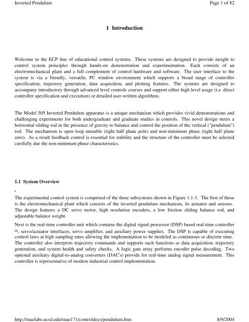
The experimental control system is comprised of the three subsystems shown in Figure 1.1-1. The first of these 

is the electromechanical plant which consists of the inverted pendulum mechanism, its actuator and sensors. 

The design features a DC servo motor, high resolution encoders, a low friction sliding balance rod, and 

adjustable balance weight. 

Next is the real-time controller unit which contains the digital signal processor (DSP) based real-time controller 

[1] , servo/actuator interfaces, servo amplifier, and auxiliary power supplies. The DSP is capable of executing 

control laws at high sampling rates allowing the implementation to be modeled as continuous or discrete time. 

The controller also interprets trajectory commands and supports such functions as data acquisition, trajectory 

generation, and system health and safety checks. A logic gate array performs encoder pulse decoding. Two 

optional auxiliary digital-to-analog converters (DAC's) provide for real-time analog signal measurement. This 

controller is representative of modern industrial control implementation. 

http://maelabs.ucsd.edu/mae171/controldocs/pendulum.htm 

8/9/2004


Electromechanical 

Apparatus 

Figure 1.1-1. The Experimental Control System 

The third subsystem is the executive program which runs on a PC under the DOS or Windows operating 

system. This menu-driven program is the user's interface to the system and supports controller specification, 

trajectory definition, data acquisition, plotting, system execution commands, and more. Controllers may 

assume a broad range of selectable block diagram topologies and dynamic order. The interface supports an 

assortment of features which provide a friendly yet powerful experimental environment. 

1.2 Manual Overview 

Real-time Controller 

Servo Amplifier 

Executive 

Software 

Page 2 of 82 

The next chapter, Chapter 2, describes the system and gives instructions for its operation. Section 2.3 contains 

important information regarding safety and is mandatory reading for all users prior to operating this equipment. 

Chapter 3 is a self-guided demonstration in which the user is easily walked through the salient system 

operations before reading all of the details in Chapter 2. A description of the system's real-time control 

implementation as well as a discussion of generic implementation issues is given in Chapter 4. Chapter 5 

presents dynamic equations useful for control modeling. Chapter 6 gives some example experiments including 

system identification, pole placement, and LQR control. Finally, Appendix A gives some details of the 

development of plant modeling equations. 


8/9/2004


2 System Description & Operating Instructions 

This chapter contains descriptions and operating instructions for the executive software and the mechanism. 

The safety instructions given in Section 2.3 must be read and understood by any user prior to operating this 

equipment. 

2.1 ECP Executive Software 

The ECP Executive program is the user's interface to the system. It is a menu driven / window environment 

that the user will find is intuitively familiar and quickly learned - see Figure 2.1-1. This software runs on an 

IBM PC or compatible computer and communicates with ECP's digital signal processor (DSP) based real-time 

controller. Its primary functions are supporting the downloading of various control algorithm parameters 

(gains), specifying command trajectories, selecting data to be acquired, and specifying how data should be 

plotted. In addition, various utility functions ranging from saving the current configuration of the Executive to 

specifying analog outputs on the auxiliary DAC's are included as menu items. 

2.1.1 The DOS Version of the Executive Program 

2.1.1.1 PC System Requirements 

Page 3 of 82 

For the ECP Executive (DOS version), you will need at least 2 megabyte of RAM and a hard disk drive with at 

least 4 megabytes of space. All DOS versions of the Executive program run under any of DOS versions 3.x, 

4.x, 5.x, and 6.x. The Executive requires a VGA monitor with a VGA graphics card installed on the PC. 

The Executive Program runs best on a 386, 486, or Pentium ® based PC with 4 megabytes or more of memory 

under DOS 5.0 or higher with HIGHMEM.SYS driver included in your CONFIG.SYS file. [2] Also, if the 

software does not "see" at least 2 megabytes of free RAM, you may find the program executing somewhat 

slowly since it will use the hard disk as virtual memory. 


8/9/2004



Page 4 of 82 

8/9/2004


2.1.1.2 Installation Procedure For The DOS Version 

The ECP Executive Program consists of several files on a 3.25" 1.44 megabyte distribution diskette in a 

compressed form. The key files on the distribution diskette are: 

ECPDYN.EXE 

ECP.DAT 

ECPBMP.DAT 

*.CFG 

*.PLT 

*.PMC 

The "ECP*.*" files are needed to run the Executive Program. The "*.CFG" and "*.PLT" files are some 

driving function configuration and plotting files that are included for the initial self-guided demonstration. The 

"*.PMC" file is the controller Personality File and should only be used in the case of a non curable system fault 

(see Utility Menu below). 

To install the Executive program, it is recommended that you make a dedicated sub directory on the hard disk 

and enter this sub directory. For example type: 

>MD ECP 

>CD ECP 

Next insert the distribution diskette in either "A:" or "B:" drive, as appropriate. Copy all files in the 

distribution diskette to the hard disk under the "ECP" sub directory. For example if the "B:" drive is used: 

>COPY B:*.* C: 

Next execute INSTALL.EXE by typing: 

>INSTALL 

You will notice some file decompression activities. This completes the installation procedure. You may run 

the ECP Dynamics Executive by typing: 

>ECPDYN 

Page 5 of 82 

The Executive program is window based with pull-down menus and dialog boxes. You may either use the 

cursor keys on the keyboard or a mouse to make selections from the pull-down menus. Vertical movement 

within these menus is accomplished by the up and down arrow keys, respectively. To make a selection with 

the keyboard, simply highlight the desired choice and press . Menu choices with highlighted letters 

may also be selected by pressing the corresponding function key. (The indicated key for menus; "alt" plus the 

indicated key within dialog boxes). 

Within dialog boxes, movement from one object to the next is accomplished by using the and the 


8/9/2004


keys. Here, "objects" includes input lines, check boxes, and "radio buttons". As you move 

from one object to the next, the selected object is highlighted. Pressing will effect the function of the 

highlighted button (e.g. termination of the dialog box will result if the Cancel button is highlighted). 

2.1.2 The Windows Version of the Executive Program 

2.1.2.1 PC System Requirements 

The ECP Executive 16-bit code runs on any PC compatible computer under Windows 3.1x and/or Windows 

95. You will need at least 8 megabyte of RAM and a hard disk drive with at least 12 megabytes of space. The 

16-bit Windows version of the Executive Program runs best with Pentium ® based PC having 16 megabytes or 

more of memory. 

2.1.2.2 Installation Procedure For The Windows Version 

The ECP Executive Program consists of several files on two 3.25" 1.44 megabyte distribution diskettes in a 

compressed form. The key files on the distribution diskettes are: 

ECPDYN.EXE 

ECP.DAT 

ECPBMP.DAT 

*.CFG 

*.PLT 

*.PMC 

The "ECP*.*" files are needed to run the Executive Program. The "*.CFG" and "*.PLT" files are some 

driving function configuration and plotting files that are included for the initial self-guided demonstration. The 

"*.PMC" file is the controller Personality File and should only be used in the case of a non curable system fault 

(see "Utility Menu" below). 

To install the Executive program enter the Windows operating system. Then go to the “Run” menu, and simply 

run the SETUP.EXE file from diskette labeled 1. Follow the interactive dialog boxes of the installation 

program until completion. 

2.1.3 Background Screen 

Page 6 of 82 

The Background Screen , shown in Figure 2.1.-1, remains in the background during system operation including 

times when other menus and dialog boxes are active. It contains the main menu and a display of real-time data, 

system status, and an Abort Control button to immediately discontinue control effort in the case of an 

emergency. 


8/9/2004


Figure 2.1-1. The Background Screen 


Page 7 of 82 

8/9/2004


2.1.3.1 Real-Time Data Display 

In the Data Display fields, the instantaneous commanded position, the encoder positions, the following errors 

(instantaneous differences between the commanded position and the actual encoder positions), and the control 

effort in volts (on the DAC) are shown. 

2.1.3.2 System Status Display 

The Control Loop Status ("Open" or "Closed"), indicates "Closed" unless an open loop trajectory is being executed 

or a "Limit Exceeded" condition has occurred. In either of these cases the Control Loop Status will indicate 

"Open". The Controller Status will indicate "Active" unless a motor over-speed, an over-travel (limit switch), or 

motor/amplifier over-temperature condition has occurred (see Section 2.3 for more details). In either of these 

cases the Controller Status will indicate "Limit Exceeded". The Limit Exceeded indicator will reoccur unless 

the user takes one of the two following actions depending on the nature of the over-limit cause. Either a stable 

controller (one that does not cause limiting conditions) must be implemented via the Control Algorithm box under 

the Setup menu or an acceptable trajectory must be executed under the Command menu. An "acceptable" 

trajectory is one that does not over-speed the motor, cause excessive travel of the sliding rod or result in 

sustained high current to the motor. The controller must be "re implemented" in order to clear the Limit 

Exceeded condition – see Section 2.1.5.1.1. 

2.1.3.3 Abort Control Button 

Also included on the Background Screen is the Abort Control button. Clicking the mouse on this button simply 

opens the control loop. This is a very useful feature in various situations including one in which a marginally 

stable or a noisy closed loop system is detected by the user and he/she wishes to discontinue control action 

immediately. Note also that control action may always be discontinued immediately by pressing the red "OFF" 

button on the control box. The latter method should be used in case of an emergency. 

2.1.3.4 Main Menu Options 

The Main menu is displayed at the top of the screen and has the following choices: 

File 

Setup 

Command 

Data 

Plotting 

Utility 


Page 8 of 82 

8/9/2004


2.1.4 File Menu 

The File menu contains the following pull-down options: 

Load Settings 

Save Settings 

About 

Exit 

2.1.4.1 The Load Settings dialog box allows the user to load a previously saved configuration file into the 

Executive. A configuration file is any file with a ".cfg" extension which has been previously saved by the 

user using Save Settings. Any "*.cfg" file can be loaded at any time. The latest loaded "*.cfg" file will 

overwrite the previous configuration settings in the ECP Executive but changes to an existing controller 

residing in the DSP real-time control card will not take place until the new controller is "implemented" – see 

Section 2.1.5.1. The configuration files include information on the control algorithm, trajectories, data 

gathering, and plotting items previously saved. To load a "*.cfg" file simply select the Load Settings command 

and when the dialog box opens, select the appropriate file from the desired directory. [3] Note that every time the 

Executive program is entered, a particular configuration file called "default.cfg" (which the user may 

customize - see below) is loaded. This file must exist in the same directory as the Executive Program in order 

for it to be automatically loaded. 

2.1.4.2 The Save Settings option allows the user to save the current control algorithm, trajectory, data gathering 

and plotting parameters for future retrieval via the Load Settings option. To save a "*.cfg" file, select the Save 

Settings option and save under an appropriately named file (e.g. "pid2.cfg"). By saving the configuration 

under a file named "default.cfg" the user creates a default configuration file which will be automatically 

loaded on reentry into the Executive program. You may tailor "default.cfg" to best fit your usage. 

2.1.4.3 Selecting About brings up a dialog box with the current version number of the Executive program. 

2.1.4.4 The Exit option brings up a verification message. Upon confirming the user's intention, the Executive 

is exited. 

2.1.5 Setup Menu 

The Setup menu contains the following pull-down options: 

Control Algorithm 

User Units 

Communications 

2.1.5.1 Setup Control Algorithm allows the entry of various control structures and control parameter values to the 

real-time controller – see Figure 2.1-2. In addition to feedforward which will be described later, the currently 

available feedback options are: 

PID 

PI With Velocity Feedback 

PID+Notch 

Dynamic Forward Path 


Page 9 of 82 

8/9/2004


Dynamic Prefilter/Return Path 

State Feedback 

General Form 

2.1.5.1.1 Discrete Time Control Specification 

Figure 2.1-2. Setup Control Algorithm Dialog Box 

Page 10 of 82 

The user chooses the desired option by selecting the appropriate "radio button" and then clicking on Setup 

Algorithm. The user must also select the sampling period which is always in multiples of 0.000884 seconds (1.1 

KHz is the maximum sampling frequency). [4] To run the selected choice on the real-time controller click on the 

Implement Algorithm button. The control action will begin immediately. To stop control action and open the loop 

with zero control effort click on the Abort button. To upload the current controller select General Form then click on 

the Upload Algorithm button followed by Setup Algorithm. Here you will find the current controller in the form that is 

actually executed in real-time – see Figure 2.1-3. 


8/9/2004


Figure 2.1-3. Dialog Box For Generalized Control Algorithm Input 

Page 11 of 82 

A typical sequence of events is as follows: Select the desired servo loop closure sampling time T s in multiples 

of 0.000884 seconds. Then select the control structure you wish to implement (e.g. radio buttons for PID, 

PID+Notch etc.). Select Setup Algorithm to input the gain parameters (coefficients). You must also select the 

desired feedback channel by choosing the correct encoder(s) used for your particular control design. Exit Setup 

by selecting OK. Now you should be back in the Setup Control Algorithm dialog box with a selected set of gains for a 

specified control structure. To download this set of control parameters to the real-time controller click on 

Implement Algorithm. This action results in an immediate running of your selected control structure on the real-time 

controller. If you notice unacceptable behavior (instability and/or excessive ringing or noise) simply click on 

Abort Control which opens up the control loop with zero control effort commanded to the actuator. 

To inspect the form by which your particular control structure is actually implemented on the real-time 

controller, simply click on Preview In General Form. You may edit the algorithm in the General Form box, however 

when you exit, you must select General Form prior to "implementing" if you want the changes to become 

effective. (i.e. the radio button will still indicate the box you were in prior to previewing and this one will be 

downloaded unless General Form is selected). 

The Setup Feed Forward option allows the user to add feedforward action to any of the above feedback structures. 

By clicking on this button a dialog box appears which allows the feedforward control parameters (coefficients) 

to be entered. To augment the feedforward action to the feedback algorithm the user must then check the 

Feedforward Selected check-box. Any subsequent downloading (via the Implement Algorithm button) combines the 

feedforward control algorithm with the selected feedback control algorithm. 

Important Note: Every time a set of control coefficients are downloaded via Implement Algorithm button, the 

commanded position as well as all of the encoder positions are reset to zero. This action is taken in order to 

prevent any instantaneous unwanted transient behavior from the controller. The control action then begins 

immediately. 


8/9/2004


Important Note: For high order control laws (those using more than 2 or 3 terms of either the R, S, T, K, or L 

polynomials), it is often important that the coefficients be entered with relatively high precision– say at least 5 

to 6 points after the decimal. The real-time controller works with 96-bit real number arithmetic (48-bit integer 

plus 48-bit fraction). Although the Executive displays the coefficients with nine points after the decimal, it 

accepts higher precision numbers and downloads them correctly. 

2.1.5.1.1 Continuous Time Control Specification 

Depending on your course of study, It may be desirable to specify the control algorithm in continuous time 

form. [5] The method for inputting control parameters is identical to that described for the discrete time case. 

Again you may preview your controller in the continuos General Form prior to implementing. Upon selecting 

either Implement Algorithm or Preview in General Form, the algorithm also gets mapped into the discrete General Form 

where it may be viewed either before (following "Preview") or after (following "Implement") downloading to the 

real time controller. [6] 

Again it is the discrete time general form that is actually executed in real time. The input coefficients are 

transformed to discrete time using one of the two following substitutions. For polynomials: n(s), d(s) in PID + 

Notch; s(s), t(s), and r(s) in Dynamic Forward Path, Dynamic Prefilter / Return Path, and the General Form; and k(s), l(s) in Feed 

Forward, the Tustin (bilinear) transform 

s = 2 

Ts 

1-z-1 

1+z -1 

is used. All other cases (first order) use the Backwards Difference method: 

s = 1-z-1 

Ts 

Blocks using the Tustin transform must be proper in s while those using backwards difference may be improper 

– e.g. a differentiator. [7] 

2.1.5.2 The User Units dialog box provides the user with various choices of angular or linear units. For Model 

505 the choices are counts, centimeters, millimeters, inches, degrees, and radians. There are 502 counts per 

centimeter travel of the sliding rod and 44.4 counts per degree (16,000 counts per revolution) of the pendulum 

rod. By clicking on the desired radio button the units are changed automatically for trajectory inputs as well as 

the Background Screen displays, plotting and jogging activities. Units of counts are used exclusively for the 

examples in this manual. 

2.1.5.3 The Communications dialog box is usually used only at the time of installation of the real-time 

controller. The choices are serial communication (RS232 mode) or PC-bus mode – see Figure 2.1-4. If your 

system was ordered for PC-bus mode of communication, you do not usually need to enter this dialog box unless 

the default address at 528 on the ISA bus is conflicting with your PC hardware. In such a case consult the 

factory for changing the appropriate jumpers on the controller. If your system was ordered for serial 

communication the default baud rate is set at 34800 bits/sec. To change the baud rate consult factory for 

changing the appropriate jumpers on the controller. You may use the Test Communication button to check data 

exchange between the PC and the real-time controller. This should be done after the correct choice of 

Communication Port has been made. The Timeout should be set as follows: 

ECP Executive For Windows with Pentium Computer: Timeout 50,000 

ECP Executive For Windows with 486 Computer: Timeout 20,000 


Page 12 of 82 

8/9/2004


ECP Executive For DOS with Pentium Computer: Timeout 150 

ECP Executive For Windows with 486 or lower Computer: Timeout 80 

2.1.6 Command Menu 

Figure 2.1-4. The Communications Dialog Box 

The Command menu contains the following pull-down options 

Trajectory Configuration 

Execute 


Page 13 of 82 

8/9/2004


2.1.6.1 The Trajectory Configuration dialog box (see Figure 2.1.-5) provides a selection of trajectories through 

which the apparatus can be maneuvered. These are: 

Step 

Ramp 

Parabolic 

Cubic 

Sinusoidal 

Sine Sweep 

User Defined 

A mathematical description of these is given later in Section 4.1. 

Figure 2.1-5. The Trajectory Configuration Dialog Box 

Page 14 of 82 

By clicking the desired radio button followed by the Setup button one selects a specific dialog box for each 

trajectory. 

The Step dialog box allows both Closed loop and Open loop step inputs. The Closed loop step subjects the closed loop 

system to a step command and is always in units of displacement (counts, inches, degrees etc.). The step size is 

incremental from the current commanded position and is always forward and backward with a specified dwell 

time and a number of repetitions. There are range limits for the maximum step size and dwell time which are 

apparatus-specific. Out-of-bounds inputs will cause an error message indicating the acceptable parameter 

range. The Open loop step [8] subjects the plant to a step input and its units are always in volts. The maximum 

voltage is +/- 3 volts. Remember that a large open loop step size combined with a large open loop dwell time 

will result in an overtravel condition which is detected by the real-time controller. This condition will cause the 

open loop step test to be aborted and the Controller Status display in the Background screen to indicate Limit Exceeded. 

To run the test again you should reduce either or both the step size and the dwell time. Also note that for very 

large closed loop step sizes the Limit Exceeded condition may occur. This is generally true for all trajectories 

whose parameters have been selected such that they generate either too large a motion or a motor/amplifier 

over-temperature (stalled) condition (see Section 2.3 on safety). 

The Ramp dialog box allows a constant speed closed loop input command. The displacement size is incremental 


8/9/2004


Page 15 of 82 

from the current commanded position and is always forward and backward with a specified speed, dwell time, 

and number of repetitions. 

The Parabolic trajectory allows a constant acceleration (quadratic in position) closed loop input command. The 

displacement size is again incremental from the current position and is always forward and backward with a 

specified acceleration time, speed, dwell time and number of repetitions. Note that the total displacement time 

may be longer than acceleration/deceleration time depending on the selected displacement size and the speed 

input. In this case the parabolic acceleration/deceleration curves are joined by a constant velocity ramp. 

The Cubic option allows a constant jerk (cubic in position) closed loop input command. As before, displacement 

size is incremental from the current position and is always forward and backward with a specified acceleration 

time, speed, dwell time and number of repetitions. Again, the total displacement time may be longer than 

acceleration/deceleration time depending on the selected displacement size and the speed input. 

Note that the only difference between a parabolic trajectory and a cubic trajectory is that, during the 

acceleration/deceleration times a constant acceleration is commanded in a parabolic input and a constant jerk 

(linearly changing acceleration) is commanded in the cubic input. Of course, in a ramp input the commanded 

acceleration/deceleration is infinite at the ends of a commanded displacement stroke and zero at all other times 

during the motion. 

The Sinusoidal dialog box provides for both Closed loop and Open loop sine wave inputs. The Closed loop option subjects 

the closed loop system to a sine wave command with amplitude in units of displacement (counts, inches, 

degrees etc.). The amplitude is incremental from the current commanded position. The user also specifies the 

frequency in Hz and the number of cycles. The open loop option specifies a sine wave input to the plant with 

amplitude in volts (at the DAC). The maximum voltage is +/- 3 volts. Remember that a open loop input to an 

unstable plant will result in an overtravel condition. Also note that very high frequency large amplitude closed 

loop tests or smaller commands near a resonant frequency result in the Limit Exceeded condition. In general, all 

trajectories which generate either too large a travel, or excessive motor power will cause this condition – see the 

safety section 2.3. These conditions will cause the open loop test to be aborted and the Controller Status display in 

the Background Screen to indicate Limit Exceeded. 

The Sine Sweep dialog box supports both Closed Loop and Open Loop sine sweep inputs. The Closed Loop option 

specifies a sine sweep in units of displacement (counts, inches, degrees etc.). The amplitude is incremental 

from the current commanded position. The user also specifies the starting and the ending frequencies in Hz and 

the sweep time. The frequency increase is linear in time. For example a sweep from 0 Hz to 10 Hz in 10 

seconds results in a one Hertz per second frequency increase. There is an apparatus-specific amplitude limit 

beyond which the Executive will not accept the inputs. The Open Loop sine sweep subjects the plant to a sine 

sweep input whose units are always in volts. The maximum voltage is +/- 3 V. Remember again that any of the 

following may result in a Limit Exceeded condition: large open loop amplitude size combined with a low 

frequency; high frequency large amplitude closed loop tests and operation near or through resonances. [9] 

The User Defined trajectory dialog box provides the interface for the input of any form of trajectory created by the 

user. In order to make use of this feature the user must first create an ASCII text file with an extension 

".trj" (e.g. "random.trj"). The content of this file should be as follows: 

The first line should provide the number of points in the trajectory. The maximum number of points is limited 

to 100. This line should not contain any other information. The subsequent lines (up to 100) should contain 


8/9/2004


the consecutive set points. For example to input twenty points equally spaced in distance one can create a file 

called "example.trj' using any text editor as follows 

20 

5 

10 

15 

20 

25 

30 

35 

40 

45 

50 

55 

60 

65 

70 

75 

80 

85 

90 

95 

100 

Page 16 of 82 

Now the segment time which is a time between each consecutive point can be changed in the dialog box. For 

example if a 100 milliseconds segment time is selected, the above trajectory would take 2 seconds to complete 

(100*20=2000 ms). The minimum segment time is restricted to five milliseconds by the real-time controller. The 

format of any ".trj" file is the same regardless of whether it was created for an open loop test or a closed loop 

test. When the points of a ".trj" file are selected for an open loop test their units are assumed to be in volts. 

For the closed loop tests the units are the current displacement units (counts, degrees, or radians). Obviously a 

user defined trajectory may also cause over-speed or over-deflection of the plant if the segment time is too short 

and the distance between the consecutive points is too long. Finally note that the closed loop user defined 

trajectories are cubic spline fitted in-between consecutive points by the real-time controller. 

2.1.6.2 The Execute dialog box (see Figure 2.1-6) is normally entered after a trajectory is selected. [10] Here the 

user has a choice of sampling the data by clicking the Sample Data check box or not sampling data by clearing the 

check box (for the details of Data Gathering see "Setup Data Acquisition" below). To move the system through the 

currently specified trajectory, click on the Run button; the trajectory will be executed by the real-time controller. 

Once finished, and provided the Sample Data check box was checked, the data will be uploaded back into the 

Executive for plotting, saving and exporting. At any time during the execution of the trajectory or during the 

uploading of data the process may be terminated by clicking on the Abort button. 


8/9/2004


2.1.7 Data Menu 

The Data menu contains the following pull-down options 

Setup Data Acquisition 

Upload Data 

Export Raw Data 

Figure 2.1-6. The Execute Dialog Box 

2.1.7.1 Setup Data Acquisition allows the user to select one or more of the following data items to be collected at a 

chosen multiple of the servo loop closure sampling period while running any of the trajectories mentioned 

above – see Figures 2.1-7 and 4.1-1: 

Commanded Position 

Encoder 1 Position 


Encoder 3 Position (not used for Model 505) 

Control Effort (output to the servo loop or the open loop command) 

Node A (input to the H polynomial in the Generalized Control Algorithm) 

Node B (input to the E polynomial in the Generalized Control Algorithm) 

Node C (output of the 1/G polynomial in the Generalized Control Algorithm) 

Page 17 of 82 

Node D (output of the feedforward controller which is added to the node C value to form the combined 

regulatory and tracking controller). 

In this dialog box the user adds or deletes any of the above items by first selecting the item, then clicking on the 

Add Item or Delete Item button. The user must also select the data gather sampling period (in multiples of the servo 

period). For example, if the sample time (T s in the Setup Control Algorithm) is 0.00442 seconds and you choose 5 for 

your gather period here, then the selected data will be gathered once every fifth sample or once every 0.0221 

seconds. Usually for trajectories with high frequency content (e.g. Step, or high frequency Sine Sweep), one 

should choose a low data gather period. On the other hand, one should avoid gathering more often (or more 

data types) than needed since the upload and plotting routines become slower as the data size increases. The 

maximum available data size (no. variables x no. samples) is 33,586. 

2.1.7.2 Selecting Upload Data allows the most recently acquired data to be uploaded into the Executive. This 

feature is useful when one wishes to switch and compare between plotting previously saved raw data and the 

currently gathered data. Remember that the data is automatically uploaded into the executive whenever a 


8/9/2004


trajectory is executed and data acquisition is enabled. However, once a previously saved raw data file is loaded 

into the Executive, the currently gathered data is overwritten. Now the Upload Data feature allows the user to 

bring the overwritten data back from the real-time controller into the Executive. 

Figure 2.1-7. The Setup Data Acquisition Dialog Box 

2.1.7.3 The Export Raw Data function allows the user to save the currently acquired data in a text file in a format 

suitable for reviewing, editing, or exporting to other engineering/scientific packages such as Matlab ® . [11] The 

first line is a text header labeling the columns followed by bracketed rows of data items gathered. The user may 

choose the file name with a default extension of ".txt" (e.g. lqrstep.txt). The first column in the file is 

sample number, the next is time, and the remaining ones are the acquired variable values. Any text editor may 

be used to view and/or edit this file. 

2.1.8 Plotting Menu 

The Plotting menu contains the following pull-down options 

Setup Plot 

Plot Data 

Print Data 

Load Plot Data 

Save Plot Data 

Close Window 

Page 18 of 82 

2.1.8.1 The Setup Plot dialog box (see Figure 2.1-8) allows up to four acquired data items to be plotted 

simultaneously – two items using the left vertical axis units, and two using the right vertical axis units [12] . More 


8/9/2004


than four items cannot appear on the same plot. Simply click on the item you wish to add to the left or the right 

axis and then click on the Add to Left Axis or Add to Right Axis buttons. You must select at least one item for the left 

axis before plotting is allowed – i.e. if only one item is plotted, it must be on the left axis. You may also change 

the plot title from the default one in this dialog box. 

Items for comparison should appear on the same axis (e.g. commanded vs. encoder position) to ensure the same 

axis scaling and bias. Items of dissimilar scaling or bias (e.g. control effort in volts and position in counts) 

should be placed on different axes. 

2.1.8.2 Plot Data generates a plot of the selected items. By clicking on the upper blue border of the plots , they 

may dragged across the screen. The view size may be maximized by clicking on the up arrow of the upper right 

hand corner. It can also be shrunk to an icon by clicking on the down arrow of the upper left hand corner. This 

function is very useful for comparing several graphs. It can be expanded back to the full size at any time by 

double-clicking on the icon. Also more than one plot may be tiled on the Background Screen [13] . By clicking on 

any point within the area of a desired plot it will appear over the others. Plots may be arbitrarily shaped by 

moving the cursor to the lower right hand corner to the position where it becomes a double-arrow . The corner 

may then be "dragged" to reshape the plot. Finally by double clicking on the top left hand corner of a plot 

screen one can close the plot window. A typical plot as seen on screen is shown in Figure 2.1-9. 

Figure 2.1-8 The Setup Plot Dialog Box (Shows case where data was gathered for encoders 1 and 2 only. Up to 20 

variables may be made available for plotting) 

Page 19 of 82 

2.1.8.3 The Axis Scaling provides for scaling of the horizontal and vertical axes for closer data inspection – both 

visually and for printing. Grid lines may be selected or deselected and data points may be labeled. 

2.1.8.4 The Print Data option allows the user to provide a hard copy of the selected plot on either an Epson 

compatible dot matrix printer or a HP Laserjet compatible printer. 

2.1.8.5 The Load Plot Data dialog box enables the user to bring into the Executive previously saved ".plt" plot 

files. Note that such files are not stored in a format suitable for use by other programs. The ".plt" plot files 


8/9/2004


contain the sampling period of the previously saved data. As a result, after plotting any previously saved plot 

files and before running a trajectory, you should check the servo loop sampling period Ts in the Setup Control 

Algorithm dialog box. If this number has been changed, then correct it. Also, check the data gathering sampling 

period in the Data Acquisition dialog box, this too may be different and need correction. 

Figure 2.1-9. A Typical Plot Window 

2.1.8.6 The Save Plot Data dialog box enables the user to save the data gathered by the controller for later 

plotting via Load Plot Data. The default extension is ".plt" under the current directory. Note that ".plt" files 

are not saved in a format suitable for use by other programs. For this purpose the user should use the Export Raw 

Data option of the Data menu. 

2.1.8.7 The Close Window option allows the currently marked plot window to close. This can also be done by 

clicking on the top left hand corner of the plot window. 

2.1.9 Utility Menu 

The Utility menu contains the following pull-down options: 

Configure Auxiliary DACs 

Jog Position 

Zero Position 

Reset Controller 

Rephase Motor 

Download Controller Personality File 

Page 20 of 82 

2.1.9.1 The Configure Auxiliary DACs dialog box (see Figure 2.1-10) enables the user to select various items for 

analog output on the two optional analog channels in front of the ECP Control Box. Using equipment such as 


8/9/2004


an oscilloscope, plotter, or spectrum analyzer the user may inspect the following items continuously in real 

time: 

Commanded Position 



Encoder 3 Position (Not used for Model 505) 

Control Effort 

Node A 

Node B 

Node C 

Node E 

Page 21 of 82 

The scale factor which divides the item can be less than 1 (one). The DACs analog output is in the range of +/- 

10 volts corresponding to +32767 to -32768 counts. For example to output the commanded position for a sine 

sweep of amplitude 2000 counts you should choose the scale factor to be 0.061 (2000/32767=0.061) This gives 

close to full +/- 10 volt reading on the analog outputs. In contrast, if the numerical value of an item is greater 

than +/- 32767 counts, for full scale reading, you must choose a scale factor of greater than one. Note that the 

above items are always in counts (not degrees or radians) within the real time controller and since the DAC's are 

16-bit wide, + 32767 counts corresponds to +9.999 volts, and -32768 counts corresponds to -10 volts. 

2.1.9.2 The Jog Position option enables the user to move the mechanism to a different commanded position. In 

contrast to displacements executed under the Trajectory dialog box, during a Jog command no data is acquired for 

plotting purposes. Since this motion is effected via the current controller, one can only jog under closed loop 

control with a stable controller. By selecting the appropriate radio button either incremental and absolute 

displacements may be carried out. The jogging feature allows the user to return to a known position after the 

execution of the various forms of open and closed loop trajectories. 

2.1.9.3 The Zero Position option enables the user to reinitialize the current position as the zero position. Note 

that if following errors exists, then the actual positions may be other than zero even though the commanded 

position is at zero (since the action is similar to commanding an instantaneous zero set point, a sudden small 

jerk in position may occur). 

2.1.9.4 The Reset Controller option allows the user to reset the real-time controller. Upon Power up and after a 

reset activity, the loop is closed with zero gains and there it behaves in the same way as in the open loop state 

with zero control effort. Thus the user should be aware that even though the Control Loop Status indicates "closed 

loop", all of the gains are zeroed after a Reset. In order to implement (or re implement) a controller you must 

go to the Setup Control Algorithm box. 


8/9/2004


Figure 2.1-10. The Configure Auxiliary DACs Dialog Box 

Page 22 of 82 

2.1.9.5 The Rephase Motor option enables the users of other ECP mechanisms to rephase their brushless motor 

commutation phase angle. This feature is not used in Model 505 with its DC brush motors. 

2.1.9.6 The Download Controller Personality File is an option which should not be used by most users. In a case 

where the real-time controller irrecoverably malfunctions, and after consulting ECP, a user may download the 

personality file if a ".pmc" file exists. In the case of Model 505, this file is named "m505.pmc". Note that 

this downloading process takes a few seconds. If the Controller Box is powered during this download process, 

this motor phasing will be effective. 


8/9/2004


2.2 Electromechanical Plant 

2.2.1 Design Description 

The plant, shown in Figure 2.2-1, consists of a pendulum rod which supports the sliding balance rod (the figure 

also serves to define the hardware terminology used throughout this manual). The balance rod is driven via a 

belt and pulley which in turn is driven by a drive shaft connected to a dc servo motor below the pendulum rod. 

Ball bearing pivot 

Rubber safety caps 

Ball 

bearing 

bushings 

Pivot 

plate 

Pendulum 

rod 

Inverted Pendulum Apparatus 

Figure 2.2-1. 

Thus by steering the sliding rod in the presence of gravity the pendulum rod angle is controlled. [14] The weight 

at the bottom may be adjusted to alter the center of gravity of the pendulum rod and (as a result) alter the system 

dynamics. An encoder position at the back of the motor senses the position and (derived) velocity of the sliding 

rod. Another encoder connected to the pivoting base of the pendulum rod is used to sense its angular position 

and velocity. 

2.2.2 Changing The Drive Belt 

Sliding rod 

Drive 

belt 

Brass "donut" 

weights (removable) 

DC servo 

motor 

Shaft encoder 

(measures x) 

Drive shaft 

(Weights and belt 

clamp not shown) 

High 

resolution 

encoder 

(measures θ) 

Brass counter masses (height 

adjustable and removable) 

Sliding rod 

limit 

switches 

Drive 

pulley 

Page 23 of 82 

In cases of heavy use or when the sliding rod contacts its travel limit under high torque, the teeth on the toothed 

belt that drives the sliding rod may become damaged. Often, the damage is of no consequence since it is 


8/9/2004


beyond the normal operating region of the sliding rod. If the damage becomes extensive though (say more than 

two adjacent teeth, or extending into the more central operating region), the belt should be replaced. 

Referring to Figure 2.2-2, the replacement procedure is as follows: 

Page 24 of 82 

1. Disconnect the drive power cable from the servo amplifier box (this is both a safety precaution and removes 

the back EMF load from the motor) 

2. With the sliding rod horizontal, use a gram force gauge to measure the friction in moving the sliding rod 

back and forth in its center (± 5 cm) of travel. (This can be done by feel alone if a force gauge is not 

available) The reading will vary, but should generally fall in the range of 40 to 70 gr. 

3. Before removing the worn belt, memorize or record how it is routed through the clamp blocks and idler and 

drive pulleys. Remove the worn belt by loosening the clamp screws on either end. 

4. Feed the new belt through the pulley system and clamp one end via the clamping block as shown in the 

lower portion of Figure 2.2-2. Be sure to firmly torque the belt clamp screws. 

5. Clamp the opposite end in its clamp block such that the belt is slightly tensioned through the pulley system 

and with 1-2 mm of clearance between the outer face of the clamp block and the end of the sliding rod. 

Firmly torque the belt clamp screws. Loosen the rod clamp screw on the same end and slide the block back 

and forth to adjust the belt tension as described in the following steps. Temporarily retighten the rod clamp 

screw when not adjusting tension. 

6. Slide the balance rod back and forth about ten times to run it in. Measure running friction as in step 2. 

Readjust belt tension if necessary to achieve a similar friction force. The pendulum will generally run better 

with less tension (hence friction) than more; however there must be enough tension so that the belt does not 

sag, disengage the pulley system, or allow the sliding rod to rotate excessively. The two clamp blocks 

should have the same angular position about the rod center-line as described in the figure. 

7. Once the tension is satisfactorily set, the any excess belt length beyond the clamps should be cut using wire 

cutters (note that the belt cable is hardened steel). 

8. Check that the four belt clamp screws and two rod clamp screws are firmly torqued before operating 

system. 

ECP supplies a spare belt with each inverted pendulum apparatus. Additional replacement belts are available 

by contacting ECP. 


8/9/2004


Sliding rod 

Toothed belt 

First insert belt in 

block and clamp this 

end (rod and belt 

calmp screws tight)... 

2.2.3 Changing Or Moving Brass Weights 

Changing Sliding Rod Drive Belt 

(see also instructions, this section) 

Figure 2.2-2. 

For safety, the following instructions must be followed faithfully whenever the weight position is changed or a 

weight is removed. 

a) Removing Or Replacing The Sliding Rod "Donut" Weights 

1) Removal or replacement is via the retaining screws (with rubber safety cap) at either end of the 

sliding rod. Make certain that the screw and safety cap are securely torqued after making any 

changes and before operating the system. This applies whether the weights are attached or not. 

2) Both donut weights must either be attached at opposite ends of the sliding rod or neither weight 

attached. Do not attach a single weight. 

b) Removing, Replacing or Changing Position Of Balance Weights 

2.3 Safety 

Idler pulleys 

Drive pulley 

... next clamp belt on block 

at this end. Then slide clamp 

block to tension belt and 

tighten rod clamp screw. 

Rod clamp 

screws (ea end) 

Clamp block (ea end) 

Belt clamp screws (ea end) 

Correct Incorrect 

Clamp blocks should be 

aligned to one another in 

the same clocking about 

the rod center line. 

1) First unlock the weights by counter-rotating them relative to each other. Then move them to the 

new desired location and relock them by firmly counter-rotating in the opposite direction. 

2) The bottom weight must have at least three threads of full engagement. 

Page 25 of 82 

3) Two, one or zero weights may be used. If a single weight is used, lock it in place using a UNF 

3/8" nut counter-rotated against the weight. 


8/9/2004


The following are safety features of the system and cautions regarding its operation. This section must be read 

and understood by all users prior to operating the system. If any material in this section is not clear to the 

reader, contact ECP for clarification before operating system. 

Important Notice: In the event of an emergency, control effort should be immediately discontinued by 

pressing the red "OFF" button on front of the control box. 

2.3.1 Hardware 

A relay circuit is installed within the Control Box which automatically turns off power to the Box whenever the 

real-time Controller (within the PC) is turned on or off. Thus for the PC bus version of the real-time Controller 

the user should turn on the computer prior to pressing on the black ON switch. This feature prevents 

uncontrolled motor response during the transient power on/off periods. The power to the Control Box may be 

turned off at any time by pressing the red OFF switch. 

Although not recommended, it will not damage the hardware to apply power to the Control Box even when the 

PC is turned off. However, doing so does not result in motor activation as the motor's current amplifier will be 

disabled. The amplifier enable signal input to the Control Box is connected to the real-time Controller via the 

60-pin flat ribbon cable. This input operates as a normally closed mode. When power to the real-time 

Controller is off, this input indicates open condition which in turn disables the motor amplifier. 

The recommended start up sequence is as follows: 

First : Turn on the PC with the real-time Controller installed in it. 

Second: Turn on the power to Control Box (press on the black switch). 

The recommended shut down is: 

First: Turn off the power to the Control Box. 

Second: Turn off the PC.. 

FUSES: There are two 3.0A 120V slow blow fuses within the Control Box. One of them is housed at the back 

of the Control Box next to the power cord plug. The second one is inside the box next to the large blue colored 

capacitor. 

2.3.2 Software 


Page 26 of 82 

8/9/2004


The Limit Exceeded indicator of the Controller Status display indicates either one or both of the following conditions 

have occurred: 

Over-travel of the sliding rod 

Over-speed of the motor. 

The real-time Controller continuously monitors the above limiting conditions in its background routine 

(intervals of time in-between higher priority tasks). In either limit case the real-time Controller opens up the 

control loop with a zero torque command sent to the actuator. The Limit Exceeded indicator stays on until a new 

set of (stabilizing) control gains are downloaded to the real-time Controller via the Implement Algorithm button of 

the Setup Control Algorithm dialog box, or a new trajectory is executed via the Command menu. Obviously the new 

trajectory must have parameters that do not cause the Limit Exceeded condition. 

Also included is a watch-dog timer. This feature provides a fail-safe shutdown to guard against software 

malfunction and under-voltage condition. The use of the watch-dog timer is transparent to the user. This 

shutdown condition turns on the red LED on the real-time Controller card. You may need to cycle the power 

to the PC in order to reinitialize the real-time Controller should a watch-dog timer shutdown occur. 

2.3.3 Safety Checking The Controller 

While it should generally be avoided, in some cases it is instructive or useful to manually contact the 

mechanism when a controller is active. This should always be done with caution and never in such a way that 

clothing or hair may be caught in the apparatus. By staying clear of the mechanism when it is moving or when 

a trajectory has been commanded, the risk of injury is greatly reduced. Being motionless, however, is not 

sufficient to assure the system is safe to contact. In some cases an unstable controller may have been 

implemented but the system may remains motionless until perturbed – then it could react violently. 

In order to eliminate the risk of injury in such an event, you should always safety check the controller prior to 

physically contacting the system. This is done by lightly grasping a slender, light object with no sharp edges 

(e.g. a ruler without sharp edges or an unsharpened pencil) and using it to slowly move the pendulum rod (See 

Fig. 2.2-1) from side to side. Keep hands clear of the mechanism while doing this and apply only light force to 

the pendulum rod. If the rod does not react violently (a safe controller will cause the system to regulate sending 

the sliding rod in a direction to counteract the disturbance) then it may be manually contacted – but with 

caution. This procedure must be repeated whenever any user interaction with the system occurs (either via the 

Executive Program or the Controller Box) if the mechanism is to be physically contacted again. 

2.3.4 Warnings 

Page 27 of 82 

WARNING #1: Stay clear of and do not touch any part of the mechanism while it is moving, while a 

trajectory has been commanded (via Execute, Command menu), or before the active controller has been 

safety checked – see Section 2.3.3. 

WARNING #2: The following apply at all times except when motor drive power is disconnected 


8/9/2004


(consult ECP if uncertain as to how to disconnect drive power): 

a) Stay clear of the mechanism while wearing loose clothing (e.g. ties, scarves and loose sleeves) and 

when hair is not kept close to the head. 

b) Keep head and face – especially eyes – well clear of the mechanism. 

Page 28 of 82 

WARNING #3: Verify that balance and sliding rod masses are secured per Section 2.2.3 of this 

manual prior to powering up the Control Box. 

WARNING #4: Do not take the cover off or physically touch the interior of the Control Box unless its 

power cord is unplugged (first press the "Off" button on the front panel) and the PC is unpowered or 

disconnected. 

WARNING #5: The power cord must be removed from the Control box prior to the replacement of 

any fuses. 


8/9/2004


3. Start-up & Self-guided Demonstration 

This chapter provides an orientation "tour" of the system for the first time user. In Section 3.1 certain hardware 

verification steps are carried out. In Section 3.2 a self-guided demonstration is provided to quickly orient the 

user with key system operations and Executive program functions. Finally, in Section 3.3, certain system 

behaviors which may be nonintuitive to a first time user are pointed out . 

All users must read and understand Section 2.3, Safety, Before performing any procedures described in this 

chapter. 

3.1 Hardware Setup Verification 

At this stage it is assumed that 

a) The ECP Executive program has been successfully installed on the PC's hard disk (see Section 2.1.2). 

b) The actual DSP printed circuit board (the real-time Controller) has been correctly inserted into an empty 

slot of the PC's extension (ISA) bus (this applies to the PC bus version only). 

c) The supplied 60-pin flat cable is connected between the J11 connector (the 60-pin connector) of the realtime 

Controller and the JMACH connector of the Control Box [15] . 

d) The other two supplied cables are connected between the Control Box and the Inverted Pendulum 

apparatus; 

e) The Inverted Pendulum apparatus has the adjustable weight at the default height shipped from the 

factory. (i.e. Plant #2 from Section 6.1) 

f) You have read the safety section 2.3. All users must read and understand that section before 

proceeding. 

Please check the cables again for proper connections. 

3.1 Hardware Verification (For PC-bus Installation) 

Step 1: Switch off power to both the PC and the Control Box. 

Page 29 of 82 

Step 2: With power still switched off to the Control Box, switch the PC power on. Enter the ECP program 

by double clicking on its icon (or type ">ECP" in the appropriate directory under DOS). You 

should see the Background Screen (see Section 2.1.3) Gently rotate the pendulum rod and later the 

top sliding rod by hand. You should observe some following errors and changes in encoder 

counts. 

Step 3: If the ECP program cannot find the real-time Controller (a pop-up message will notify you if this is 

the case), try the Communication dialog box under the Setup menu. Select PC-bus at address 528, and 

click on the test button. If the real-time Controller is still not found, try increasing the timeout in 


8/9/2004


20 ms increments up to a maximum of 300 ms. If this doesn't correct the problem, switch off power to your 

PC and then take its cover off. With the cover removed check again for the proper insertion of the 

Controller card. Switch the power on again and observe the two LED lights on the Controller 

card. If the green LED comes on all is well; if the red LED is illuminated, you should contact ECP 

for further instructions. If the green LED comes on, turn off power to your PC, replace the cover 

and turn the power back on again. Now go back to the ECP program and you should see the 

positions change as you gently move the pendulum rod. 

Step 4: Make sure that you can rotate the pendulum rod and move the sliding rod freely. Now connect the 

power cord to the Control Box and press the black "ON" button to turn on the power to the Control 

Box. You should notice the green power indicator LED lit, but the motor should remain in a 

disabled state. Do not touch the apparatus any more, remember whenever power is applied to the 

Control Box there is a potential for uncontrolled motion of the pendulum (see the warnings in 

Section 2.3). 

Step 5: Now turn off the power to your PC. 

Page 30 of 82 

This completes the hardware verification procedure. Please refer again to Section 2.3 for future start up and 

shut down procedures. 


8/9/2004


3.2 Demonstration Of The Apparatus And ECP Executive Program 

Page 31 of 82 

This section walks the user through the salient functions of the system. By following the instructions below you 

will actually implement a controller, maneuver the system through various trajectories, and acquire and plot 

data. 

Step 1: With the power to the Control box turned off, enter the ECP Executive program. You should see 

the Background Display. Turn on power to the Control Box (press on the black button). Now 

enter the File menu, choose the Load Setting option and select the file default.cfg. This 

configuration file is supplied on the distribution diskette and should have been copied into the ECP 

directory by now. Note that this file would have been loaded into the Executive automatically (see 

Section 2.1.4.1). This particular default.cfg file contains the controller gain parameters and 

other trajectory, data gathering and plotting parameters specifically saved for the activities within 

this section. 

This file has been created to operate with a plant which has the adjustable weight at the factory default setting. 

It could generate an unstable response if the position of the adjustable weight on the lead screw is significantly 

altered. 

Step 2: Enter the Utility menu and Reset the controller. Place the sliding rod in its approximate center of 

travel. With aid of an object such as a ruler, balance the pendulum rod so that it remains vertical 

(see Fig. 3.2-1). If the pendulum remains balanced without support, you may proceed to the next 

step without holding it up. Otherwise you may need to manually keep it vertical with the ruler (so 

that you can stay clear of the mechanism). Be sure to keep your head clearly away from the 

mechanism and out of the plane of action of the sliding rod. 

Step 3: Now enter the Setup menu and choose, Setup Control Algorithm option. You should see the sampling 

time T s = 0.00884 seconds, Discrete time control, and the General Form button selected. Now select Setup 

Algorithm and you should see the following gains: T 0 =2.5, S 0 =24.61, S 1 =-24.00, H 0 =1,0 I 0 =1.8427, I 1 =- 

1.76, E 0 =0.35, and G 1 =-0.5. This controller was designed using the linear quadratic regulator (LQR) 

technique with all error weighting on encoder #1 (the pendulum angle encoder). In addition, a low 

pass filter was included (G 1 coefficient) to reduce quantization noise. 


8/9/2004


Balance Rod near 

center of travel 

Equilibrium Position For Beginning Demo 

Pendulum Rod approx vertical 

Figure 3.2-1 

Exit this dialog box and, with the pendulum in the vertical position and the sliding rod in its 

middle "T" position, select Implement Algorithm. The control law is now downloaded to the real-time 

Controller. Very gently push the pendulum rod with the ruler to verify that control action is in 

effect (see Sect. 2.3.3, "Safety Checking The Controller") If you do not notice any motor power, 

use the ruler to move it back to the vertical position and then, click on the Implement Algorithm button 

again until you notice the servo loop closed. Now select Upload Algorithm, then General Form and Setup 

Algorithm. You should see the same coefficients uploaded back from the real-time controller to the 

Executive program. Note that the general form algorithm is the only structure that actually runs in 

real-time. All other structures (e.g. PID etc.) are translated to the general form by the Executive 

prior to implementation. 

Step 4: Enter the Data menu and select Setup Data Acquisition. In this box make sure that the following four 

items are selected: Commanded Position and Encoders 1,2, & Control effort. Data sample period 

should be 5 which means that data will be collected every fifth servo cycle (in this case every 

5*0.00884 seconds). Now exit this menu. 

Step 5: Enter the Command menu and select Trajectory. In this box select Step and then Setup. You should see 

step size = 300 counts, dwell time =4000 ms and no. of repetitions = 1. If not, change the values to 

this parameter set. Exit this box and go to the Command menu. This time select Execute and with the 

Sample Data box checked run the trajectory. You should have noticed a step move of 300 counts, a 

dwell of 4 second and a return step move. Wait for the data to be uploaded from the real-time 

Controller to the Executive program running on the PC. Now enter the Plotting menu and choose 

Setup Plot. Select Encoder 1 and Commanded Position for plotting (left axis) and select Plot Data. 

Page 32 of 82 

You should see a plot similar to the one shown in Figure 3.2-2. Replace Encoder 1 with 2 via the 

Setup Plot box and then plot data. A similar plot to the one shown in Figures 3.2-3 should be seen. 

Notice the initial reverse motion which is a characteristic of a non-minimum phase plant. This 

phenomenon is explained from basic laws of dynamics. 


8/9/2004


You may re-position the plots by dragging the upper plot frame bar. Try shrinking the second plot 

by clicking on the down arrow on the top right hand corner. A minimized plot may be expanded at 

any time by double-clicking on its icon. Clicking on the top right hand upward arrow expands the 

plot to full size. (It must be brought back to normal size however prior to shrinking.) You can resize 

the plots using the cursor to "drag" the lower right hand corner of the plot frame (position 

cursor at corner and begin "dragging" when cursor becomes double arrow). 

Figure 3.2-2 Step Response at Angle Encoder (#1) 

Figure 3.2-3 Step Response at Sliding Rod Encoder (#2) 

Page 33 of 82 

Step 6: Enter the Command menu and select Trajectory. In this box select Parabolic and then Setup to enter the 

Ramp dialog box. You should see distance = 300 counts, velocity = 1000 counts/s, dwell time 

=4000 ms and no. of repetitions = 1. If not, change the values to this set. Exit this box and go to 

the Command menu. Now select Execute and with Sample Data checked, run the trajectory and wait for 

the data to be uploaded from the real-time Controller. You should have noticed the ramp move 

(constant acceleration to top speed) of 300 counts followed by a dwell of 4 seconds and then the 

reverse motion.. Now enter the Plotting menu and choose Setup Plot. Select Encoder 1 and 

Commanded Position for plotting and then plot the data. You should see a plot similar to the one 

shown in Figure 3.2-4. Note that the initial reverse motion is smaller in amplitude. You may save 

the ramp or the step response under anyname.plt using the Save Plot Data option. Any plot data 

thus saved may be reloaded from the disk using the Load Plot Data option for future inspection, 

plotting or printing. To print simply choose the Print Data menu option and select the appropriate 


8/9/2004


printer before the printing command. Alternatively, any set of collected data may be exported as an ASCII 

text file by way of the Export Data option of the Data menu. 

Now try Parabolic and Cubic trajectories all default amplitudes should be 300 counts. Compare 

commanded and actual velocities of encoder 1 under these trajectories. Many conclusions can be 

drawn regarding the nature of the actual motion based upon the commanded trajectory profiles. 

Now close all plot windows. 

If the sinusoidal trajectory is selected, the default values of amplitude and frequency should be 

200 counts and 0.5 Hz respectively with 10 repetitions selected. Executing this and plotting the 

response should yield a graph similar to the one shown in Figure 3.2-5. Note the amplitude 

attenuation and the phase lag. 

Figure 3.2-4 Ramp Response at Encoder 1 

Figure 3.2-5 Sinusoidal Response at Encoder 1 (0.5 Hz) 

Page 34 of 82 

Step 6: Again enter Trajectory and select Sine Sweep then Setup. You should see the amplitude = 175 counts, 

max. freq.= 6 Hz, min. freq.= 0.1 Hz and the sweep time = 29.5 sec. Again, if different, change the 

values to correspond this set. While running this trajectory, you should notice sinusoidal motion 

with increasing frequency for one minute. Now enter the Plotting menu and choose Setup Plot. This 

time select only Encoder 1 for plotting and then plot the data. You should see a plot similar to the 


8/9/2004


one shown in Figure 3.2-6. 

Figure 3.2-6 Sine Sweep Response at Encoder 1 (Pendulum Angle Encoder) 

3.3 Nonintuitive System Behavior 

Page 35 of 82 

An explanation of system functionality which may be nonintuitive to first time (or first few time) users is given 

below. 

Point 1: Upon PC power up, the control loop is closed but all gains are cleared to zero. As a result, even 

though the status display indicates CLOSED LOOP, the control effort is zero indicating that there is 

no force demand from the actuator. With zero gains, the closed loop system behaves like an 

open loop one. This initialization of the gains to zero also takes place every time the real-time 

controller is Reset under the Utility menu. 

Point 2 Even though the parameters for a particular control algorithm may exist within the Executive, 

the real-time Controller does not carry them until the Implement Algorithm button of the Setup Control 

Algorithm dialog box is activated. Then the control is implemented immediately 

Point 3 The Limit Exceeded message comes on as a result of either motor over-speed or sliding rod 

over travel. In either case the message does not clear until a stable set of control gains are 

downloaded or a less abrupt trajectory is requested (see Section 2.1.3 ). Also if the control box is 

turned off, the Limit Exceeded message may be shown even when the sliding rod is not in 

contact with the limits. 


8/9/2004


4. Real-Time Control Implementation 

This chapter is a description of the real-time controller functionality and a tutorial on related implementation 

issues. 

The ECP real-time Controller is a Digital Signal Processor (DSP) based single board computer which executes 

the following real-time tasks: 

Servo loop closure 

Command generation 

Brush motor commutation (not applicable to Model 505) 

Sensor Interface 

In addition, in the background (while not executing the above tasks) it carries out the following: 

User Interface via PC and/or RS232 Bus 

Limits and Safety Activities 

4.1 Servo Loop Closure 

Servo loop closure involves computing the control algorithm at the sampling time. The real-time Controller 

executes the General Form equation of the control law at each sample period T s . This period can be as short as 

0.000884 seconds (approx. 1.1 KHz) or any multiple of this number. The Executive program's Setup Control 

Algorithm dialog box allows the user to alter the sampling period. All forms of control laws are automatically 

translated by the Executive program to the General Form prior to downloading ("implementing") to the 

Controller. The General Form uses 96-bit real number (48-bit integer and 48-bit fractional) arithmetic for the 

computation of the control effort. The control effort is saturated in software at +/- 16384 to represent +/- 5 volts 

on the 16-bit DACs whose range is +/- 10 volts. The +/-5 volt limitation is due to the actuator 's amplifier input 

voltage scaling. 

Referring to Figure 4.1-1, the control equations are as follows: 

R(q -1 )nodeA(k) = T(q -1 )*c p (k)-S(q -1 )*f b1 (k) 

Page 36 of 82 

Here T ,S , and R are seventh order polynomials of the unit time shift operator q, and the letter k represents the 

k th sampling period for k=0, 1,2, ... . The variable nodeA is an intermediate value 


8/9/2004


of the overall control law equation which is stored in the memory and may be acquired by the user through the 

Data Acquisition feature of the Executive program. The variable c p (k) is the commanded position which is 

generated by the real-time Controller as described in the next section. The variable f b1 (k) may be from any of 

the three possible feedback sensors depending on the state of software loop switch 1. 


Figure 4.1-1. General Form Of The ECP Control Algorithm 

Page 37 of 82 

8/9/2004


Next the intermediate loop is computed as follows 

J(q -1 )*nodeB(k) = H(q -1 )*nodeA(k)-I(q -1 )*f b2 (k) 

Here again nodeB is an intermediate value stored in the memory and f b2 is the sensor feedback selected via loop 

switch 2. J, H, and I are second order polynomials. For the inner loop we have 

G(q -1 )*nodeC(k) = E(q -1 )*nodeB(k)-F(q -1 )*f b3 (k) 

NodeC is the contribution to the value of the control effort generated by the overall regulator and f b3 is the 

sensor feedback selected via loop switch 3. G, E, and F are second order polynomials. For the feedforward 

loop we have 

L(q -1 )*nodeD(k) = K(q -1 )*cp(k) 

In this case nodeD is the contribution to the value of the control effort generated by the feedforward terms, L 

and K are sixth order polynomials. 

The combined regulatory and tracking controller generates the control effort as: 

control effort(k) = nodeC(k)+nodeD(k) 

The general control structure described above supports the implementation of a broad range of specific control 

forms. 

4.2 Command Generation 

Command generation is the real-time generation of motion trajectories specified by the user. The parameters of 

these trajectories are downloaded to the real-time Controller through the Executive program via the Trajectory 

Configuration dialog box. This section describes the trajectories generated in the current control version. 

4.2.1 Step Move 

Figure 4.2-1a shows a step move demand. The desired trajectory for such a move can be described by 

c p (t) = c p (0)+C for t >0 

c v (t)=0 for t >0 

c v (0)=∞ 

Page 38 of 82 

Where c p (t) and c v (t) represent commanded position and velocity at time t respectively and C is the constant 

step amplitude. Such a move demand generates a strong impulsive torque from the control actuator. The 

response of a mechanical system connected to the actuator would depend on the dynamic characteristics of the 

controller and the system itself. However, in a step move, the instantaneous velocity and its derivatives are not 


8/9/2004


directly controllable. Usually step moves are used only for test purposes; more gentle trajectories are nearly 

always used for practical maneuvers. 

4.2.2 Ramp Move 

A ramp demand is seen in Figure 4.2-1b. The trajectory can be described by 

c p (t) = c p (0)+V*t for t >0 

c v (t) = V for t >0 

c a (0) = ∞ 

where c a (0) represents commanded acceleration at time zero and V is a constant velocity. Relative to a step 

demand, a ramp demand is more gentle, however the acceleration is still impulsive. The commanded velocity is 

a known constant during the maneuver. 

4.2.3 Parabolic Move 

Figure 4.2-1c shows a parabolic move demand. Its trajectory can be expressed as: 

c p (t) = c p (0)+c v (0)*t+1/2 A*t 2 for t >0 0 0 0 0 0


Figure 4.2-1. Geometric Command Trajectories Of Increasing Order 


Page 40 of 82 

8/9/2004


4.2.5 The Blended Move 

Any time a ramp, a parabolic or a cubic trajectory move is demanded the real-time Controller executes a general 

blended move to produce the desired reference input to the control algorithm. The move is broken into five 

segments as shown in the velocity profile of Figure 4.2-2. For each section a cubic (in position) trajectory is 

planned. Five distinct cubic equations can describe the forward motion . After the dwell time, the reverse 

motion can be described by five more cubic trajectories. Each cubic has the form:. 

cp (t)= cp (0)+V *t+1/2 A *t i i i i 2 3 +1/6 J *t i = 1,...,5 

i 

Using a known set of trajectory data (i.e. the requested total travel distance, acceleration time t acc, and the 

maximum speed v max , for each move), the constant coefficients V i, , A i , and J i are determined for each segment 

of the move by the real-time Controller. This function is known as the "motion planning" task. Note that for a 

parabolic profile J i =0, and for a ramp profile A i is also zero which further simplifies the task. Having 

determined the coefficients for each section, the real-time Controller uses these values at the servo loop 

sampling periods to update the commanded position (reference input). For example if the segment is a cubic (J 

0): 

c a (k)= c a (k-1) +J*T s 

c v (k)=c v (k-1)+c a (k)*T s 

c p (k)=c p (k-1)+c v (k)*T s 

where T s is the sampling period and c a (k), c v (k), c p (k) represent commanded acceleration, velocity and position 

at the k th sampling period. 

4.2.6 Sinusoidal Move 

Figure 4.2-2 Velocity Profile for General Blended Move 

The sinusoidal move is generated using the following equation: 

c p (k)= R* sin (θ(k)) 


Page 41 of 82 

8/9/2004


where R is the amplitude, θ(k)=ω*k*T p for k=0,1,..., and ω is the commanded frequency in Hz. T p is set to five 

milliseconds. To further smooth out the trajectory, a cubic spline is fitted between the points as follows: 

c p '(k)= (c p (k-1)+4*c p (k)+c p (k+1))/6 

For the linear sine sweep, ω(k) = α*T p , where α is a constant determined by the difference between the 

maximum and the minimum frequency divided by the sweep time 

α =(ω max - ω min ) / sweep time 

4.3 Brush Type DC Servo Motor and Drive Amplifier 

The control effort at the k th sampling period is the input to a 16-bit DAC which provides an analog signal for the 

motor amplifier. The amplifier operates in a transconductance mode providing a current (as opposed to voltage) 

demand to the motor which in turn represents a torque demand from the motor. To provide the current source 

capability an analog proportional plus integral (PI) controller is implemented within the amplifier for tracking 

the demanded current. Referring to the block diagram of Fig. 4.3-1, the transfer function between the motor 

current and the DAC output (control effort) is given by: 

i(s) 

u(s) = 

(4.3-1) 

Here k c is the DAC gain in volts/count (10 volts per 32767 counts), k A is the amplifier forward gain which is 

dimensionless (V/V), R is the motor armature and brush resistance in ohms, L is the motor armature inductance 

in henrys, k b is the motor back emf constant in v/(rad/s), k t is the motor torque constant in Nm/ampere, k m is the 

mechanical advantage constant which is the ratio of the force generated by the belt driving the sliding rod to the 

torque generated by the motor (N/Nm), and G(s) is the transfer function between current and the motor velocity. 

In current mode drive amplifier, both the proportional gain k p and the integral gain k i of the amplifier are chosen 

to be very high relative the inner back emf loop within the practical range of motor operation. As a result, the 

effect of the inner loop may be ignored and the transfer function may be simplified to: 

At steady state this transfer function becomes: 

i(s) 

u(s) 

kAkc kps+ki 

s Ls+R+ktkbG(s) + kps+ki 

i(s) 

u(s) = 

kAkc kps+ki 

s Ls+R + kps+ki 

= kAkc 

The force delivered to the sliding rod at steady state then becomes: 

F(s) 

= kAkckTkm 

u(s) 


(4.3-2) 

(4.3-3) 

(4.3-4) 

Page 42 of 82 

8/9/2004


In general, the analog PI controller gains of the amplifier are such that the dynamics of the current loop are 

much faster relative to the dynamics of the motor and mechanical plant. As a result the steady state value of 

current is achieved virtually instantaneously relative to changes in velocities and positions. Thus in this 

transconductance (current feedback) mode, the combined amplifier/ motor combination can be though of as a 

force generator with the characteristic of gain value k f . The specific value of k f for the Model 505 apparatus is 

given in Chapter 6 Experiment #1. 

Controller 

Voltage proportional 

to desired 

output 

current 

ui 

kc 

"u(s)" 

kA u*(s) 

DAC 

Servo Amplifier 

4.4 Multi-Tasking Environment 

- 

kp + ki 

s 

Voltage propor- 

tional to motor 

current 

v 

- 

Motor drive dynamics 

Mechanism Drive Block Diagram 

Figure 4.3-1. 

Digital control implementation is intimately coupled with the hardware and software that supports it. Nowhere 

is this more apparent than in the architecture and timing used to support the various data processing routines. A 

well prioritized time multi-tasking scheme is essential to maximizing the performance attainable from the 

processing resources. 

The priority scheme for the ECP real-time Controller's multi-tasking environment is tabulated in Table 4.4-1. 

The task with the highest priority is the commutation algorithm which takes place at the rate of 9.049 kHz 

(since the motor is not brushless, this algorithm is bypassed in the case of Model 505 system). The next highest 

priority task is the trajectory update and servo loop closure computation which takes place at the maximum rate 

of 1.131 KHz (minimum sampling period is 0.000884 seconds). In this case, the user may reduce the sampling 

rate through the Executive Program via changes to T s in the Setup Control Algorithm dialog box. 

The trajectory planning task has the third highest priority and is serviced at a maximum rate of 377 Hz. Here 

the parameters for a new trajectory need not be calculated every time this task is serviced by the real-time 

Controller. Whenever a new trajectory is required (i.e. the current trajectory is near its completion) this task is 

executed. The lower priority tasks are system house keeping routines including safety checks, interface and 

optional auxiliary analog output. 

Back 

EMF 


1 

kb 

Shaft 

speed 

ω 

Motor admittance 

1 

Ls+ R 

Plant 

dynamics 

i 

G(s) 

Torquec 

constant 

k T 

T 

kc 

F 

Page 43 of 82 

8/9/2004


Table 4.4-1 The Multi-Tasking Scheme of the Real-Time Controller 

Priority Task Description Service Frequency 

1 Commutation (not Executed for Model 505) 9.049 KHz 

2 Servo Loop Closure & Command Update 1.1 KHz 

3 Trajectory Planning 377 Hz 

4 Background Tasks including User Interface, 

Auxiliary DAC Update, Limit checks etc. 

Background (In time between 

other tasks) 

Page 44 of 82 

The higher priority tasks always prevail over lower ones in obtaining the computational power of the DSP. This 

multi-tasking scheme is realized by a real-time clock which generates processor interrupts. 


8/9/2004


4.5 Sensors 

There are two incremental rotary shaft encoders used in the inverted pendulum . These are used to sense the 

position and velocity of the pendulum rod and the sliding rod. The pendulum angle encoder has a resolution of 

4000 counts per revolution. The sliding rod encoder (connected to the motor) has a resolution of 500 counts per 

revolution which is equivalent to approximately 12500 counts per meter of the sliding rod travel. (the actual 

sliding rod travels approximately 0.24 meter). 

The encoders are all optical type whose principle of operation is depicted in Figure 4.5-1. A low power light 

source is used to generate two 90 degrees out of phase sinusoidal signals on the detectors as the moving plate 

rotates with respect to the stationary plate. These signals are then squared up and amplified in order to generate 

quadrate logic level signals suitable for input to the programmable gate array on the real-time Controller. The 

gate array uses the A and B channel phasing to decode direction and detects the rising and falling edge of each 

to generate 4x resolution – see Figure 4.5-2. (Hence the effective encoder resolution is 16,000 counts/rev. and 

50200 counts/m for the respective pendulum and balance rod measurements.) The pulses are accumulated 

continuously within 24-bit counters (hardware registers). The contents of the counters are read by the DSP once 

every servo (or commutation) cycle time and extended to 48-bit word length for high precision numerical 

processing. 

Figure 4.5-1 The Operating Principle of Optical Incremental Encoders 


Page 45 of 82 

8/9/2004


4.6 Auxiliary Analog Output (system option) 

Figure 4.5-2. Optical Encoder Output 

There are two analog output channels in the Control Box which are connected to two 16-bit DACs which 

physically reside on the real-time Controller. Each analog output has the range of +/- 10 volts (-32768 to 

+32767 counts) with respect to the analog ground. The outputs on these DACs are updated by the real-time 

Controller as a low priority task. However, for most trajectories (e.g. for sine sweep up to approx. 25 Hz ), the 

update rate is sufficiently fast for an oscilloscope inspection of the Controller's internal signals. See the section 

on the Executive Program's Utility menu for the available signals to output on these DACs. 

5. Plant Dynamic Models 

Page 46 of 82 

This Chapter provides time domain expressions which are useful for nonlinear plant modeling and Laplace 

domain expressions useful for linear control implementation. These are used in the experiments described later 

in this manual. A discussion of generic control issues relating to this plant type is provided in Appendix B. 


8/9/2004


5.1 Equations of Motion 

5.1.1 Nonlinear Expressions 

Neglecting friction effects, the plant may be modeled as shown in Fig. 5.1-1 [16] . From the figure we have that 

the system kinetic energy, T(s) is: 

T = 1 

2 m1vcg1 

2 + 1 

2 

J1θ + 

2 1 

2 m2vcg2 

2 + 1 

2 

J2θ 

2 

g 

θ 

cg2 

α 

l m1 

x 

u1 

u2 

cg1 

a) Whole Plant 

g 

Includes Motor & 

Counter Mass 

θ 

m2 

Plant Model Descriptions 


O 

l c 

F(t) 

J2 

l o 

m1 

x 

J 1 

F(t) 

b) Two Principal Structural Members 

(5.1-1) 

Page 47 of 82 

Figure 5.1-1 

8/9/2004


where the v cg 's are the inertial velocities of the respective members' centers of gravity (c.g's) (see Fig. 5.1-1b) 

and the J i 's are the polar moments of inertia about the respective c.g's. The members are kinematically 

constrained so that: 

(5.1-2) 

(5.1-3) 

where the underscored quantities are treated as vectors and "x" is the vector cross product. By resolving unto 

the u1 and u2 components and squaring, it is readily shown that: 

(5.1-4) 

Substituting Eq's 5.1-3,-4 into 5.1-1 and using: lm1 2 2 2 

= l +x and cos α = l /lm1 yields: 

o 

o 

where 

Jo(x) = J1 +J2 + m1 lo (5.1-6) 

2 +x2 + m2lc 2 

is the system moment of inertia about O. 

The potential energy, V, taken with the datum at {θ=90 o , x=0} is: 

= m1 g lo cosθ -xsinθ + m2 glccosθ (5.1-7) 

To obtain the equations of motion, we use Lagrange's equation in the form: 

(5.1-8) 

(5.1-5) 

where q i is the i th generalized coordinate, and Q i is the associated generalized force [17] . Choosing q 1 =x, q 2 =θ, we 

have: 

vcg1 = x + θ xlm1 

vcg2 

= lcθ 

2 

2 vcg1 = 2 

x + lm1 θ + 2 lm1xθ cosα 

T = 1 

2 J1 +J2 + m1 lo 2 +x 2 + m2lc 2 θ 2 

+ 1 

2 m1x 2 + m1loxθ 

= 1 

2 

Jo(x)θ + 

2 1 

2 m1x 2 + m1loxθ 

V = m1 glm1 cos(θ +α) + m2 glccosθ 

= m1 glm1 cosθ cosα - sinθsinα + m2 glccosθ 

∂ 

∂t 

∂T 

∂qi 

- ∂T 

+ 

∂qi 

∂V 

∂qi 

= Qi 

m1x+m1loθ - m1xθ 2 - m1gsinθ = F(t) 

m1lox+Joθ +2m1xxθ - (m1l0 + m2lc)gsinθ - m1gxcosθ = 0 


(5.1-9) 

(5.1-10) 

Page 48 of 82 

8/9/2004


These equations are useful for nonlinear system design and analysis. For example, when linear control is 

implemented based on a linearized plant model, the system time response with the full-term (nonlinear) and 

linearized plants may be simulated to evaluate the range of validity of the linear approximation. The simulation 

with nonlinear plant model may then be compared with actual test results on the ECP system to see the effects 

of further unmodeled and non-ideal dynamic behavior. [18] 

5.1.2 Linearization About Equilibrium 

The equilibrium points x=x e , θ=θ e , may be found from Eq's 5.1-8 & -9 by solving for the motionless system ( 

) when F(t) = 0. These are readily obtained as: [19] 

x=x=θ=θ =0 

θ e = 0, x e = 0 (5.1-11) 

A linearized approximation of the system may be found via the first two (zeroeth and first order) terms of the 

Taylor's series expansion about the equilibrium points [20] . This results in: 

where: 

5.1.3 State Space Realization 

(5.1-12) 

Isolating the second derivative terms in equations 5.1-12,-13 we have: 

Joe (5.1-15) 

-m1lo 2 θ - m1gx -m2lcgθ = -F(t)lo 

By inspection, a state space realization of the linearized plant is: 

where: 

m1x+m1loθ - m1gθ = F(t) 

m1lox+Joeθ - (m1l0 + m2lc)gθ - m1gx = 0 

Joe = Jo x=xe 

θ=θe 

Joe -m1lo 2 x + m1logx - Joe - m1lo 2 -m2lolc gθ = F(t)Joe 

m1 

x = Ax + BF(t) 

Y= Cx 

(5.1-16) 


(5.1-13) 

(5.1-14) 

Page 49 of 82 

8/9/2004


and 

x = 

B = 1 

J * 

(5.1-17) 

C i = 1 (i=1,2,3,4) when x i is an output and equals 0 otherwise. 

5.1.4 Transfer Function 

θ 

θ 

x 

x 

, A = 

0 

-lo 

0 

Joe /m1 

J * = Joe-m1lo 2 

By Laplace transform of Eq. (5.1-13) and assuming zero valued initial conditions it is straightforward to express 

θ(s) 

x(s) 

s (5.1-18) 

2- m1lo+m2lc g/Joe 

which when substituted into Eq. (5.1-12) leads to: 

θ(s) 

F(s) 

= m1lo 

Joe 

, C = 

-s 2 + g/lo 

0 1 0 0 

m2lcg/J * 0 m1 g/J * 0 

0 0 0 1 

J * -m2lolc g/J * 0 -m1log/J * 0 

C 1 0 0 0 

0 C2 0 0 

0 0 C3 0 

0 0 0 C4 

(5.1-19) 

The first of the above transfer functions relates the motion of the nominally vertical (or pendulum) rod to the 

motion of the sliding rod and the second relates pendulum rod motion to the force acting on the sliding rod via 

the drive belt. It is the motion of the pendulum rod (i.e. θ) that is to be controlled in the experiments that 

follow. 

The linearized relationship between the applied force and the sliding rod position follows from the product of 

Eq.(5.1-19) and the inverse of Eq. (5.1-18): 

x(s) 

F(s) 

= lo 

J * 

= Joe 

m1J * 

-s2+ g/lo 

s4+ m1lo-m2lc g/J * s2 - m1g2/J * 

s2- m1lo+m2lc g/Joe 

s4+ m1lo-m2lc g/J * s2 - m1g2/J * 


, 

(5.1-20) 

Page 50 of 82 

8/9/2004


5.2 Effect Of Mass Properties & Geometry On Plant Dynamics 

Page 51 of 82 

From inspection of Eq. 5.1-19, it is readily seen that the transfer function of the linearized plant has one right 

half plane (RHP) zero and at least one RHP pole. Thus the open loop system is both nonminimum phase and 

unstable. As will be discussed later, these characteristics have strong implications to the attainable performance 

and stability of any subsequent closed loop design. In particular, the nonminimum phase zero sets an upper 

limit to the achievable system bandwidth, and the unstable pole sets a lower limit. These properties are 

discussed in more detail in Appendix A. The effects of various dynamic parameters on the values of the plant 

transfer function roots are described in this section. 


8/9/2004


5.2.1 Distribution And Effect Of Zeros 

From Eq 5.1-19, the zeros lie at: 

(5.2-1) 

Thus for the experimental plant the zeros are fixed since the pendulum rod length, l o , is not changeable. From 

the discussions of Appendix A, the lower the "frequency" (magnitude) of the RHP zero, the lower the maximum 

attainable closed loop bandwidth, and hence performance. From the Appendix, for practical control 

implementation, we would not expect to attain closed loop bandwidths greater than about (g/l o ) 1/2 or 1.2 Hz for 

our particular geometry. 

5.2.2 Distribution And Effect Of Poles 

In order to gain insight as to the effect of mass properties on the distribution of the poles, consider the following 

notation: 

Note that since: 

(5.2-2) 

(5.2-3) 

(5.2-4) 

(5.2-5) 

b>0 and k>0. Equation 5.1-19 may then be expressed as: 

or: 

(5.2-6) 

(5.2-7) 

where: (5.2-8) 

p1 = -a + a2 +4b (>0) 

2 

and 

z = ± g/lo 

a = ∆ m1lo - m2lc / J * 

b = ∆ m1 / J * 

k = ∆ lo / J * 

J * = Joe - m1lo 2 = J1+J2+m2lc 2 (>0) 

θ(s) 

F(s) = -k s2 + g/lo 

s 4 + ags 2 - bg 2 

θ(s) 

F(s) = 

-k s 2 + g/lo 

s 2 -p1g s 2 -p2g 


Page 52 of 82 

8/9/2004


p2 = -a - a2 +4b 

2 

(


Equations 5.2-7,8,&9 show that their are two real poles at ± 

possible pole-zero distributions are shown in Figure 5.2-1. 

p1 g and two imaginary poles at ± i p2 g. 

Two 

x o 

Figure 5.2-1. Possible Pole-Zero Distributions 

According to Eq's 5.2-1,-7,&-8, the distribution of Figure 5.2-1a implies that: 

-a + a2+4b 

2 

(5.2-10) 

It is relatively straightforward to show that this holds if and only if: 

J * < m2lclo 

o x 

(5.2-11) 

Similarly, the distribution of Fig. 5.2-1b implies that: 

J * > m2lclo 

x 

x 

a) | Real Poles | > | Zeros | b) | Real Poles | < | Zeros | 

> 1 lo 

Im Im 

Re 

(5.2-12) 

Eq. 5.2-11 is equivalent to the condition that J 1 +J 2 +m 2 (l c ) 2 < m 2 l c l o . This in turn requires that J 1 and J 2 be small 

and l c be small relative to l o . It can be shown that for the range of available parameters, this condition is never 

realized in the experimental system. Therefore, all pole-zero distributions are as shown in Figure 5.2-1b. Note 

also from Eq’s 5.2-8,-9 that the magnitude (frequency) of the imaginary poles is always greater than the real 

poles. 

For the experimental system, the masses m 1 and m 2 may be changed discretely by adding or removing the 

appropriate brass weights and by changing the distance of the balance weight along the lead screw from the 

pivot. The effect of these changes is shown in Figure 5.2-2. From the discussions of Appendix A, the lower the 

frequency of the unstable pole, the less difficult it is to stabilize the system under closed loop control. As seen 


o x 

x 

x 

x 

o 

Re 

Page 54 of 82 

8/9/2004


in the Figure, stabilizing the system becomes less difficult when the balance masses are added, when they are 

moved as far downward as possible, [21] and when the "donut" weights on the sliding rod are removed. [22] 

The case where both balance masses are removed altogether is nearly identical to the left most points on the 

curves of Figure 5.2-2a. From the discussion of Appendix A this would be a difficult plant to stabilize indeed. 

Pole or Zero Frequency (rad/s) 

101 

Transfer Function Roots With One Pendulum Balance Mass 

Zeros (real & opposite signed) 

Imag poles – no "donut "mass on m 1 

Imag poles – with "donut" mass on m 1 

Real poles – no "donut" mass on m 1 

Real poles – with "donut" mass on m 1 

Physical limit of balance mass position 

100 

0 0.05 0.1 0.15 0.2 

Negative Of Distance From Pivot To Balance Mass c.g. (m) 

Figure 5.2-2a. Effect of Changing Plant Mass Properties - Single Balance Mass 


Page 55 of 82 

8/9/2004


Pole or Zero Frequency (rad/s) 

101 

Figure 5.2-2a. Effect of Changing Plant Mass Properties - Two Balance Masses 

5.2.3 Mass Property Determination. 

100 

0 0.05 0.1 0.15 0.2 

Both the nonlinear (Eq's 5.1-9,-10) and linearized (Eq's 5.1-12) time domain equations of motion and the 

transfer function (Eq. 5.1-19 or Eq's 5.2-6,-7) are fully specified by the parameters m 1 , m 2 , l o , l c , and J * . For the 

experimental pendulum (and for a given set of attached brass weights), the parameters m 1 , m 2 and l o are fixed 

and known. The parameters l c , and J * however depend on the location of the movable brass counter-mass. 

Define l co and m 2o to be the value of l c and m 2 respectively when the counter-mass, m w2 , (both brass weights) is 

removed. Then the parameter l c is found from a simple center of mass calculation, i.e.: 

lc = mw2lw2+m20lco 

m2 

Transfer Function Roots With Two Pendulum Balance Masses 

Zeros (real & opposite signed) 

Imag poles – no "donut "mass on m 1 

Imag poles – with "donut" mass on m 1 

Real poles – no "donut" mass on m 1 

Real poles – with "donut" mass on m 1 

Physical limit of balance mass position 

Negative Of Distance From Pivot To Balance Mass c.g. (m) 

(5.2-13) 

where l w2 is the distance (signed) from the pivot to the center of m w2 . 

In our case, the parameters l co and m 2o are also fixed and known so that determination of l c is straightforward. 

The remaining parameter J * is found experimentally [23] as described in Chapter 6. 


Page 56 of 82 

8/9/2004


6 . E x p e r i m e n t s 

This chapter outlines experiments which identify the plant parameters, implement several control schemes, and 

demonstrate important control principles. The versatility of this software / hardware system allows for a 

broader range of experimental uses than will be described here and the user is encouraged to explore whatever 

topics and methodologies may be of interest – subject of course to your school and laboratory guidelines and 

the safety notations of this manual. The safety portion of this manual, Section 2.4, must be read and understood 

by any user prior to operating this equipment. 

The instructions in this chapter begin at a high level of detail so that they may be followed without a great deal 

of familiarity with the PC system interface and become more abbreviated in details of system operation as the 

chapter progresses. To become more familiar with these operations, it is strongly recommended that the user 

read Chapter 2 prior to undertaking the operations described here. Remember here, as always, it is 

recommended to save data and control configuration files regularly to avoid undue work loss should a system 

fault occur. 

6.1 System Identification 

It is necessary to identify pertinent dynamic and scaling parameters in order to design and implement controllers 

which stabilize the inverted pendulum plant and allow it to track set-points in angular displacement. In Chapter 

5 the nonlinear dynamical equations of the plant were derived. A linearized model of the plant dynamics was 

also presented in both state-space form and transfer function form. The linearized model can be shown to be an 

adequate representation in many cases for the purpose of linear control design and implementation (e.g. the 

controller used as the default controller in Section 3.2 uses a linear controller designed based upon this 

linearized model). The purpose of the proceeding identification procedures will be to provide numerical values 

for the symbolic equations derived in Chapter 5. It is recognized that not all parameters may be measured with 

a fully assembled pendulum. As result, Table 6.1-1 below shows the parameters which are fixed. Their 

nominal values have been measured prior to assembly: 

Table 6.1-1. Mass Property Values 

Parameter Value Description 

lo 0.330 (m) Length of pendulum rod from pivot to the sliding rod T section 

m1 TBD † m1o (kg) 

0.103 (kg) 

Mass of the complete sliding rod including all attached elements. 

Mass of the sliding rod with belt, belt clamps, and rubber end 

guards (but without sliding rod brass "donut" weights) 

mw1 0.110 (kg) Combined mass of both of the sliding rod brass "donut" weights 

(=0 if not used) 

m2 TBD (kg) Mass of the complete assembly minus m1 http://maelabs.ucsd.edu/mae171/controldocs/pendulum.htm 

Page 57 of 82 

8/9/2004


m w2 

† To be determined 

From the definitions in the table we have: 

The parameter 

1.000 (kg) 

(÷2 if only one 

weight used) 

Mass of brass balance weight 

m 2o 0.785 (kg) Mass of the complete moving assembly minus m 1 and m w2 

l co 0.071 (m) Position of c.g. of the complete pendulum assembly with the 

sliding rod and balance weight removed 

Jo * 0.0246 (kg-m 2 ) 

m 1 = m 1o + m w1 (6.1-1) 

m 2 = m 2o + m w2 (6.1-2) 

lw2 = signed distance from pivot to c.g. of balance mass (m ) w2 ∆ 

is changeable by the user and is readily measured. That is, referring to Figure 6.1-1, 

(6.1-3) 

The three remaining parameters – J * ,J oe, and l c – are derived from the above as follows: 

lc = mw2lw2+m20lco 

m2 

J * = Joe-m1lo 2 

2 

[J -m l ] evaluated when mw2 =0. 

oe 1 o 

lw2 = - t+lt +lb 

2 

(5.2-13) 

Joe = Jo * + mllo 2 + mw2 lw2 2 

(5.1-17) 


(6.1-4) 

Page 58 of 82 

8/9/2004


DC servo 

motor 

Plant Configurations For Control Experimentation. 

t 

l b 

Figure 6.1-1 Measurement of l w2 

High resolution 

encoder 

Counter 

mass 

The experiments that follow in this manual use two distinct physical setups and corresponding parameter sets 

for their models. In each case both "donut" weights are used for the sliding rod and both balance masses are 

used . For the first case, "Plant #1", l t = 10.0 cm, and for the second ("Plant #2") l t = 7.0 cm, . 

Based upon the above information you should now be able to calculate the numerical values of the linearized 

plant parameters as given by Eq’s 5.1-18, -19, and -20 in Chapter 5. Calculate these values for each plant case. 

Calculate the roots of the transfer function Eq 5.1-19 and show that the real poles and zeros are mirror images 

about the imaginary axis on the s-plane and that there is also an imaginary pole pair. Show that the poles of Eq. 

5.1-18 are imaginary for plant #1 and are real and opposite for plant #2. [24] 

Now we can use the numerical value of plant transfer function or state space model to design controllers. 

However to actually implement them we need four scaling parameters which are associated with the 

amplifier/actuator, the two sensors (encoders) and the controller firmware. With reference to the block diagram 

of Figure 6.1-2, these four scale factors (gains) are as shown in Table 6.1-2 where θ c and x c are the respective 

values of θ and x in units of encoder counts. [25] 

Now, all of the above parameters are fixed. The value of k f is factory set and will not change unless the 

amplifier analog gains are changed. The value of k x comes from the fact that encoder 2 generates 2000 counts 

per revolution which translates to approximately 50,000 counts per one meter travel of the sliding rod (after 4x 

interpolation, see Section 4.5). Similarly, k a is reflects the 16,000 counts per rev. resolution of encoder 1. The 

value of k s is fixed by the firmware within the real-time control card. 

Construct the properly scaled plant models (with variables θ c and x c and control force F c ) in both transfer 

function and state space form (i.e. Eq's 5.1-16, -18, -19, and -20) by using the following substitutions. [26] 


l t 

Page 59 of 82 

8/9/2004


Scale 

Factor 

k f 

k x 

k a 

k s 

θ = θ c / (k s k a ) (6.1-5) 

x = xc / (ks k ) (6.1-6) 

x 

F = F k (6.1-7) 

c f 

Table 6.1-2. Scaling Constants 

Value Description 

0.0013 (N / DAC increment) Combined DAC-amplifier-motor-pulley gain (see Sect. 4.3) 

50200 (increment / m) Sliding rod encoder (encoder 2) scale factor 

2546 (increment / rad) Pendulum angle encoder (encoder 1) scale factor 

32 (controller or DAC incr../ 

encoder or demand incr..) 

Control 

Effort 

ks Controller kf 

u(t) 

Time Domain 

DSP controller firmware scale factor 

Control 

Effort 

ks Controller 

kf 

u(s) 

Laplace Domain 

Linearized Plant Model 

x = Ax + Bu 

y = Cx 


xc 

θc 

Motor encoder - pulley 

xc 

θc 

kx 

Pivot encoder 

ka 

x(s) 

F(s) 

kx 

ka 

θ 

x 

Linearized Plant Model 

Motor encoder - pulley 

Pivot encoder 

x θ(s) 

x(s) 

θ 

Page 60 of 82 

Figure 6.1-2 

8/9/2004


6.1.1 Confirmation of k a and k x 

Plant Block Diagram With Scale Factors 

These two scale factors can be easily confirmed via a simple procedure using the Executive program 

Procedure 

1. Remove the power cord from the control box but have all other cables connected. Position the pendulum 

rod to the right and the sliding rod to the far right at the limit of travel. Enter the Executive program. 

2. Select Zero Position in the Utility menu. You should see the position of Encoder 1 and Encoder 2 to be 

approximately zero. 

3 Hold on to the pendulum rod and push the sliding rod from one end until it hits the opposite end of its travel 

(hits the right limit switch). Now record the number of counts moved by encoder 2 on the Background Screen. 

With a ruler, measure the distance in meters that the sliding rod has traveled from one limit switch to the 

other. The ratio of the two is the value of k x . 

4. Now move the pendulum rod in the anti-clockwise direction all the way to the left. Record the number of 

counts moved by encoder 1 on the Background Screen. Measure the angle of rotation in radians, the ratio of the 

two is the value of k a . 

6.1.2 Confirmation of 

The following procedure may be used to confirm the value of from which J * and J oe are obtained via Eq's 

6.1-4 and 5.1-17 

Procedure: 

Jo * 

1. Remove the brass balance weights from the apparatus and install both "donut" weights on the sliding rod. 

Use a rubber band to restrain the sliding rod in its center of travel as shown in Figure 6.1-2. 

2. Disconnect the power cord from the control box but leave the other cables connected. (This allows the 

encoder signals to pass to the control card but precludes accidental driving of the motor.) Very carefully 

position the entire pendulum mechanism up-side down on two coplanar flat surfaces such that the 

pendulum rod is free to rotate as a non-inverted (regular) pendulum. (E.g. two tables side-by-side with 

approx. 8 in. gap between. It is recommended that a piece of cloth or other soft material be placed between 

the mechanism and the table on each side to avoid scratching.) 


Jo * 

Page 61 of 82 

8/9/2004


Use rubber band to 

restrain sliding rod in 

center position 

Figure 6.1-2. Securing Sliding rod For Jo Measurement via Pendulum Frequency 

* 

3. With the controller powered up , enter the Control Algorithm box via the Set-up menu and set T s = 0.00442. Go 

to Set up Data Acquisition in the Data menu and select encoder #1 as data to acquire and specify data sampling every 

5 servo cycles (i.e. every 5 T s 's). Select OK to exit. With the pendulum hanging freely under gravity, select 

Zero Position from the Utility menu to zero the encoder positions. 

4. Check again that the pendulum rod can freely rotate in this position. Now select Trajectory in the Command 

menu. Enter the Step dialog box and click on step-up. Choosing Open loop Step, input a step size of 0 (zero), a 

duration of 10000 ms and repetition of 1. Exit to the Background Screen by consecutively selecting OK. 

This puts the controller in a mode for acquiring 20 sec of data on command but without driving the 

actuator. This procedure may be repeated and the duration adjusted to vary the data acquisition period. 

5. Select Execute from the Command menu. Manually displace the pendulum rod approximately 20 deg. from 

vertical and let go. You should notice that the "non-inverted" pendulum rod will oscillate and slowly 

attenuate while the encoder data is collected to record this response. Select OK after data is uploaded. 

6. Select Set-up Plot from the Plotting menu and choose encoder #1 position; then select Plot Data from the Plotting 

menu. You should see the pendulum rod angle encoder response similar to one shown in Figure 6.1-2. 

Figure 6.1-2 Determination of via Pendulum Period Measurement 

Jo * 

Page 62 of 82 

7. Measure the period of oscillation, T, in seconds by taking the time for completion of several cycles divided 

by the number of cycles. Confirm that its value for the factory default setting of the balance weight (all the 

way down the lead screw but just clearing the pocket hole) is approximately 1.25 seconds [27] . Use the 

following classic linearized "non-inverted" equation of motion to derive an expression for the inertia J in 

terms of the measured T. 


8/9/2004


Jθ + mlcggθ = 0 

(6.1-8) 

where m, J and l cg are the respective mass, inertia, and length to center of gravity (from the pivot) of the 

combined pendulum elements during the test. 

8. Calculate the values of m and l cg for the test case and hence obtain J from your derived expression. (Note 

that J here is the same as J of this manual's notation) Now determine oe 

hence verify the value shown in Table 6.1-1. 

according to = J-m l 1 o 

9. Carefully re-orient the mechanism to the regular "inverted pendulum" position (up-side up) and reconnect 

the power cord to the control box. (Make certain that the control box is turned off however.) This 

concludes the confirmation procedure for J * . 

From the above exercises all plant parameters and scaling constants have been found or verified. 

6.2 Successive Loop Closure / Pole Placement Design 

In this experiment we first close the loop about the "x" position with a relatively high bandwidth (close 

tracking) PD control. We then make the assumption that the sliding rod closely follows its internal demand u x 

so that for designing a controller for θ, the "plant" is approximated by the transfer function θ c (s)/x c (s) (i.e. the 

scaled version of Eq. 5.1-18). The block diagram for this approach is given in Figure 6.2-3. 

6.2.1 PD Control Of The Sliding Rod 

A simplified dynamical model of the relationship between the sliding rod and the applied force, F when the 

plant is at the equilibrium position is shown in Figure 6.2-1. Here the inertia of the pendulum assembly is 

* 

shown as an equivalent mass m at the sliding rod interface according to: 

2 

* * 2 m = J / lo 

(6.2-1) 

2 


Jo * Jo * 

Page 63 of 82 

2 and 

8/9/2004


Figure 6.2-1 Simplified Model Of Sliding Rod Dynamics When Plant Is At Equilibrium 

The reader should verify that the following relationship holds for the motion x(t): 

where 

(6.2-2) 

(6.2-3) 

Thus the reduced dynamics are that of a simple rigid body. For our particular plant, the corresponding transfer 

function in controller units is: 

where 

F(t) = m * x 

m * = m1m 2 * 

m1 +m 2 * 

xc(s) khw = 

Fc(s) m* 1 s2 khw = ∆ kxkskf 

x 2 (t) 

x(t) 

(6.2-4) 

(6.2-5) 

m 1 

F(t) 

m 2 * 

Page 64 of 82 

The block diagram of the proportional plus derivative (PD) control of a rigid body is shown in Figure 6.2-2 and 

has the closed loop transfer function: [28] 


8/9/2004


By defining: 

we may express: 

Figure 6.2-2. Rigid Body PID Control – Control Block Diagram 

(6.2-7) 

(6.2-8) 

(6.2-9) 

Here ω n is the natural frequency and ζ is the damping ratio of the closed loop system x(s)/F(s). 

Procedure : 

c(s) = 

(6.2-6) 

x(s) 

r(s) = 

khw/m* 1 kds+kp 

s2 + khw/m* 1 kds+kp 

ωn = ∆ 

PD Control 

r(s) 

Reference 

input 

∆ kdkhw ζ = 

2m * ωn 

Σ 

kpkhw 

m * 

– 

kdkhw 

= 

2 m * kpkhw 

c(s) = 2ζωns +ωn 2 

s 2 +2ζωns +ωn 2 

k p + k d s 

Controller 

khw 

Hardware 

Gain 

1 

m * s 2 

1. Using the results of Section 6.1 for Plant #1 determine the values of the parameters k hw and 

* 

m . 1 

2. Using Equations 6.2-7 and -8, determine values of the control parameters k and k to provide 

p d 

a closed loop natural frequency of 10 Hz (63 rad/s) and damping ratio of 1 (critically 

damped). Note: if you obtain 0.15 < k < 0.35 or 0.004 < k < 0.012 you should check and 

p d 

correct your calculations. 

3. Adjust the position of the balance masses to l t = 10.0 cm being sure to secure them on the 

threaded rod by counter rotating them. Verify that the donut weights are in place and secure 

on the sliding rod. Hence place the apparatus in the Plant #1 configuration. 

4. In the Executive program, set-up to collect Encoder #2 and Commanded Position information via the 


Plant 

x(s) 

Sliding rod 

position relative 

to pendulum rod 

end 

Page 65 of 82 

8/9/2004


Set-up Data Acquisition box in the Data menu with data sampling every two sample periods. Enter the 

Command menu, go to Trajectory and select Step, Set-up. Select Closed Loop Step and input a step 

size of 1000 counts, a duration of 1000 ms and 1 repetition. Exit to the Background Screen 

by consecutively selecting OK. This puts the controller board firmware in a mode to command 

a 1000 count step move (about 2 cm.) forward and back with a one second dwell. 

5. Enter the Control Algorithm box under Set-up and set Ts=0.00442 s and select Continuous Time Control. 

Select PID and Set-up Algorithm. Enter the k p and k d values (k i = 0) determined in step 2 (again, do 

not enter values outside of the ranges 0.15 < k p < 0.35 or 0.004 < k d < 0.012) and select 

Encoder #2 for feedback, then OK. 

Orient the mechanism with the sliding rod in its approximate middle of travel so that the 

pendulum rod is approximately vertical. In this and all future work, be sure to stay clear of 

the mechanism before doing the next step. Selecting Implement Algorithm immediately 

implements the specified controller; if there is an instability or large control signal [29] , the 

plant may react violently. If the system appears stable after implementing the controller, first 

displace it with a light, non sharp object (e.g. a plastic ruler) to verify stability prior to 

touching plant. AT ALL TIMES KEEP HEAD AND ESPECIALLY EYES WELL CLEAR 

OF THE APPARATUS 

Select Implement Algorithm, then OK. 

6. Enter Execute under Command and – again staying clear of the apparatus –select Run. You should 

see the sliding rod move rapidly about 2 cm back and forth while the pendulum rod swings 

due to the reactive force. 

7. Plot encoder #2 output and commanded position, both on the left axis (see step 6, Section 

6.1.2). You should see a critically damped response with 90% rise time of approximately 60 

ms. Print your plot via Print Data under the Plotting menu. 

6.2.2 Pole Placement Control of θ(s)/x(s) 

Page 66 of 82 

Having closed a relatively high bandwidth ( 10 Hz) loop about the sliding rod position we utilize the fact that 

the transfer function of Eq. 6.2-9 has near unity input/output gain (and near zero phase) through the bandwidth 

( 0.75 Hz) that we will attempt to attain in the overall control of θ. Thus for the control of θ we consider the 

block diagram of Figure 6.2-3. [30] 


8/9/2004


rc(s) kpf e*(s) 

x θc(s) 

Σ Σ k c(s) x 

c 

p + k 

c(s) θc(s) 

ds 

R (s) 

Fc(s) 

xc(s) Now the plant to be controlled is: 

θc(s) 

xc(s) 

= kam1lo 

kxJoe 

Control Structure For Outer Loop Closure 

(6.2-10) 

Figure 6.2-3. 

where the obvious substitutions are made in obtaining the right hand expression. The numerical values of the 

parameters in this expression were determined in Experiment #1. 

We now seek to find a controller S(s)/R(s) which will result in a prescribed set of closed loop poles. The closed 

loop denominator will have the form: 

Dcl(s) = Dax(s)R(s) + k (6.2-11) 

* Nax(s)S(s) 

which may be expressed as [31] 

– 

where the d i 's and n i 's are known from the plant model Eq. 6.2-10 

– 

-s 2 + g/lo 

S (s) 

R(s) 

s 2 - m1lo+m2lc g/Joe 

c(s) = 

= ∆ k *Nax(s) 

Dax(s) 

x c(s) 

e*(s) 

Dcl(s) = (d2s 2 + d1s+ d0)(r1s+ r0) + (n2s 2 + n1s+ n0)(s1s+ s0) 


- 1 (through control bandwidth) 

(6.2-12) 

Page 67 of 82 

8/9/2004


By linear system theory, for coprime N ax (s), D ax (s) with N ax (s)/D ax (s) proper, there exists an (n-1) th order S(s), R 

(s) which when convolved as per Eq. (6.2-11) form an arbitrary (2n-1) th order D cl (s) where n is the order of D ax 

(s). 

Here we shall solve for the desired denominator: 

Dcl(s) = (s+π+jπ)(s+π-jπ)(s+3π) (6.2-13) 

I.e. closed loop poles at -0.5 ± j0.5 and -1.5 Hz. 

Procedure : 

Pole Placement Control 

1. Determine the coefficients of the controller polynomials S(s) and R(s) by equating coefficients 

in the expanded forms of Eq's 6.2-12 and 6.2-13. 

2. Calculate the scalar prefilter gain k pfc by referring to Figure 6.2-3 and Eq. 5.1-18 using the 

scaled variable set θ c, and x c, . The goal is to have the output θ c (s) (or θ(s)) scaled equal to the 

input r c (s) (or r(s)) Hint: Consider the system in static equilibrium. Set θ c =1 and r c = 1; 

determine the required input x c (s) to the plant θ c (s) / x c (s) and hence the necessary signal at 

the left hand input to the left most summing junction in Figure 6.2-3. 

4. In the Executive program, set-up to collect Encoder #1, Encoder #2 and Commanded Position information 

[32] via Set-up Data Acquisition with data sampling every two sample periods. Enter the Command 

menu, go to Trajectory and select Step, Set-up. Select Closed Loop Step and input a step size of 

500 counts, a duration of 2500 ms and 1 repetition. Exit to the Background Screen by 

consecutively selecting OK. This puts the controller board firmware in a mode to command a 

500 count step move (about 11 deg.) forward and back with a 2.5 second dwell. 

5. Enter the Control Algorithm box under Set-up and set [33] Ts=0.00884 s and select Continuous Time 

Control. Select General Form and Set-up Algorithm and enter the k p and k d values (k i = 0) from the 

previous section (Section 6.2.1) as the coefficients e o and e 1 respectively. Enter the 

coefficients for S(s) and R(s) determined in step1. Enter the value k pf calculated in step 2 as t o 

in the General Form. Make sure that Encoder #1 is selected for Loop #1 and Encoder #2 for 

Loop #2. Select OK to exit to the controller selection dialog box. 

6. Always do the following to avoid transients when implementing your controller. Exit to the 

background screen. Select Abort Control to make certain that the pendulum is safe to touch. Set 

the sliding rod at its approximate center of travel (pendulum rod approximately vertical). 

Check that the controller box is powered on and turn on if it is not. Select Reset Controller from 

the Utility menu. Do not disturb the pendulum. 

7. Reenter the Control Algorithm box and while staying clear of the mechanism select Implement 

Algorithm. If the pendulum reacts violently you have implemented an unstable controller or 

otherwise improperly entered the control coefficients and you will need to repeat the above 

steps as appropriate. If the pendulum is well behaved you may (again, while staying clear of 


Page 68 of 82 

8/9/2004


the pendulum) perturb the pendulum rod gently with a long blunt object such as a ruler. You 

should see the sliding rod move in an attempt to regulate against the disturbance. You may 

notice some "twitching" or buzzing due to noise in the system. This is to be expected. The 

time under closed loop control should be minimized however to reduce the stress on the drive 

components (In the next experiment, a filter is designed to reduce the noise.) 

8. Enter Jog Position under Utility and input an absolute jog of -250 counts. You should see the 

pendulum move clockwise about 5.5 degrees. 


Page 69 of 82 

8/9/2004


9. Enter Execute under Command and – again staying clear of the apparatus –select Run. You should 

see the pendulum – actuated by the sliding rod – move rapidly about 11 deg back and forth. 

Open the loop by selecting "Abort Control". 

10. Plot encoder #1 output and commanded position, both on the left axis. Note the initial 

negative going motion of the pendulum. This is a time response characteristic of 

nonminimum phase systems. Print your plot via Print Data under the Plotting menu. Save your 

control configuration via Save Settings in the File menu. 

6.3 Low Pass Filter Augmentation Of Controller 

It may have been noticed in the previous experiment that the pendulum appeared to "jitter" or "twitch" as a 

result of quantization noise which is always amplified by numerical differentiation. To overcome this problem 

a low pass filter may be used which should have a break frequency much higher than the closed loop bandwidth 

(so that system stability is not significantly affected) and yet low enough to effectively attenuate the noise. In 

this section we shall investigate the effect of a simple first order lag with unity dc gain. 

Procedure 

1. Verify that a first order filter represented by the transfer function G(s) = 1/(τs+1) has a lowpass 

frequency response with bandwidth 1/τ (rad/s). 

2. Consider the filter given by: 

G(s) = 1/(0.008s+1) 

What is the cut-off frequency of this filter and how does its value compare to the magnitude of 

the closed loop poles of the design in the previous section? 

3. To implement this filter as a cascade to the output of the control blocks used in Section 6.2, 

we must use the General Form structure within the Setup Control Algorithm Dialog Box. Enter the 

ECP Executive program and in Setup Control Algorithm, enter the sampling period T s =0.001768 [34] . 

Input control coefficients in the General Form box from the design of Section 6.2 (you may do 

this quickly by uploading your saved configuration from the last experiment via Load Settings in 

the File menu – make sure however that you choose T s =0.001768) Now input g1= 0.008, g0=1. 

This corresponds to the implementation of the above first order low pass filter to the output of 

the control action from the PD inner loop (i.e. immediately prior to the control signal output 

from the controller and being put on the DAC). Now exit the General form box and after 

following the instructions of step 6 of Section 6.2.2 and staying clear of the mechanism, 

Implement the algorithm. You should see a considerable reduction in jittering (i.e. numerical 

noise) from your previous controller's operation. Why should this filter be implemented to the 

output as opposed to the input of the controller? Remember it is the numerical noise that we 


Page 70 of 82 

8/9/2004


are trying to attenuate not sensor noise. Is sensor noise a source of concern with optical shaft 

encoders as used in the pendulum mechanism? Execute and plot a step response as per steps 

4, 6,7,8, 9, and 10 of Section 6.2.2. 

4. Repeat the procedures in steps 2 & 3 reducing the time constant of the filter progressively (e.g. 

to 75% of its existing value each time) from 0.008 seconds keeping sampling time the same. 

You should note that as the time constant gets smaller the effect of filter fades away. Why? 

5. Repeat the procedure in steps 2 & 3 increasing the time constant of the filter (e.g. by 150%) 

progressively from 0.008 seconds keeping the sampling time the same. You should notice 

that as the time constant of the filter gets larger it starts to affect the underlying dynamic 

response by increasing the response time to a step input, overshoots and finally instability. 

Why? 

6.4 Pole Placement Controller For Unstable θ(s)/x(s) 

For Plant #1, the denominator of θ(s)/x(s) has left half plane roots and is stable [35] . The physical interpretation 

is that the system c.g. is below the pivot so that if the sliding rod were fixed, the mechanism would behave as an 

ordinary (noninverted) pendulum. In Plant #2, however, the balance masses are raised bringing the c.g. above 

the pivot and θ(s)/x(s) is unstable. Stabilizing and controlling such a system graphically demonstrates the 

effectiveness of closed loop control. 

Procedure: 

1. Adjust the position of the balance masses to l t = 7.0 cm being sure to secure them on the 

threaded rod by counter rotating them. Verify that the donut weights are in place and secure 

on the sliding rod. Hence place the apparatus in the Plant #2 configuration. 

2. Repeat the design and implementation process of Section 6.2, noting the following: 

a) You may assume that the PD controller designed previously (Section 6.2.1) has similar 

natural frequency and damping (you may verify this by recalculating m * and then ω n and 

ζ for the new mass properties) when applied here and hence you may use the same k p & 

k d . 

b) Use the same desired closed loop denominator given by Eq. (6.2-13). 

c) In initializing the system per step 6 in Section 6.2.2 it will be more difficult to manually 

balance the pendulum such that you Reset Controller then Implement Algorithm without the 

pendulum moving. With a little practice however you should be able to do it. 

3 You should add a noise filter to your design per Section 6.3 before implementing. 

4. Compare your step response with that obtained in Section 6.2. How do the closed loop 

transfer functions compare? (Assume that c(s)=1 throughout the control bandwidth.) 


Page 71 of 82 

8/9/2004


5. Save your controller configuration via Save Settings in the File menu. 

6.5 LQR Control Design 

Since the open loop pendulum mechanism (Plant #2 configuration) is both naturally unstable and non-minimum 

phase it would be difficult (if not impossible) to implement controllers which only use the angle sensor as 

feedback (e.g. PD control of pendulum angle). In this section, full state feedback control of the pendulum 

mechanism based upon the linearized model is addressed. LQR synthesis via the Riccati equation solution or 

numerical synthesis algorithms is used to find the state feedback controller gains which minimize the cost 

function (scalar control effort): 

J = ∨ (x ' Qx + Ru 2 ) dt (6.4-1) 

Carry out the LQR design as follows: 

Procedure 

1. Construct the numerical value of the state space model of Eq. 5.1-16 using the Plant #2 model from Section 

6.1 (with variables θ c and x c and control force F c ). 

2. Choose the output vector C to be a row vector equal to [1 0 0 0] which defines the pendulum angle to be the 

single output. Choose Q=C ' *C which means that pendulum angle error as the error to be minimized subject 

to the control effort cost. 

3. Choose the control weighting function R to range between R = 5.0 to R = 50. Remember the smaller the 

value of R (control effort weight) the higher the value of gains and potentially the higher the bandwidth. 

However too small a value of R can cause unacceptable demand on the actuator and almost always causes 

excessive noise in the system. Can you explain why? 

4. Perform LQR synthesis via the Riccati equation or otherwise to obtain a state feedback gain vector K, given 

by [k 1 k 2 k 3 k 4 ], such that the feedback law is: 

u(t)= -K x(t) 

For each value of R determine the gain vector K. Here, since the state space plant has already been scaled 

in controller units, the values for K are themselves scaled for direct input in the real time controller. 

5. Verify that two of the closed loop poles determined from the eigenvalues of [A-BK] approach the negative 

real zero of the open loop plant as R reduces. Also, the other two poles increase in magnitude and tend 

toward 135 and 225 degrees in the complex plane as R is reduced. Is this result consistent with the theory 

of the asymptotic behavior of LQR controllers? Explain. 

8. Now we determine the prefilter gain working on commanded position such that the steady state value of the 

actual angle corresponds to the commanded angle. Using closed loop transfer function with full state 

feedback, show that the value of commanded angle position θ d must be pre-scaled by the following 

expression for zero steady state error: 

r c = [-m 1* g/(k a *k s *k f ) - k x *((m 1 l o +m 2 l c )/(m 1 *k a ))*k 3 +k 1 ]*θ d (6.4-2) 


Page 72 of 82 

8/9/2004


Here the signal r c is the output of the prefilter gain in the state feedback control scheme. Remember that k 1 

is the gain feedback from the pendulum rod angle position sensor and k 3 is the gain feedback from the 

sliding rod position sensor. 

Determine the value of the quantity [-m 1* g/(k a *k s *k f ) - k x *((m 1 l o +m 2 l c )/(m 1 *k a ))*k 1 +k 3 ]. Carry out this task 

for each value of the gain set determined for each value of R. i.e. for each value of R, determine: 

k pf = [-m 1* g/(k a *k s *k f ) - k x *((m 1 l o +m 2 l c )/(m 1 *k a ))*k 3 +k 1 ] (6.2-8) 

Page 73 of 82 

9. You are should now be ready to implement these state feedback controllers and observe these respective 

behaviors. Turn off power to the Control Box. Enter the ECP Executive program and select the Setup 

menu. Click on Control Algorithm and then choose Continuous time, then State Feedback and Setup Algorithm. Using the 

state feedback structure enter the scaled prefilter k pf gain determined in step 9. Enter the scaled values of k 1 

(for encoder 1 position), k 2 (for encoder 1 velocity), k 3 (for encoder 2 position) and k 4 (for encoder 2 

velocity) for the value of gains determined for R=50. Choose the sampling period T s to be 0.00442 

seconds. Now manually move the pendulum rod to the vertical position and the sliding rod to the middle 

position to balance the apparatus (this may take a little practice). Complete the initialization and 

implementation procedure described in Steps 6 and 7 of Section 6.2.2 keeping your hands and head well 

away from the mechanism. You should see a stable response. Gently disturb the pendulum rod (not the 

sliding rod) with a slender blunt object (such as a ruler) and note that as for the other controllers, it attempts 

to servo back to its original position. 

10. If a stable response results, go to the Data menu and select commanded position, encoder 1 & 2 positions 

and control effort with a sample period of 5 servo cycles. Go to Jog Position under the Utility menu and "jog" 

to the -200 count position. Exit this menu and enter the Command menu. Select Step and then Setup. Choose 

Closed Loop with step size of 400 counts and a dwell time of 4000 ms with one repetition. Exit this menu 

and choose Command followed by (with Sample Data box checked) Execute. Plot and print your response data. 

11. Repeat steps 9 & 10 for each gain set corresponding to the value of R=50 to 5.0. Note that as R gets 

smaller, gains get larger and the response becomes faster. However at higher gains the system appears to 

make a buzzing sound associated with sensor quantization noise. The system should not be ran for longer 

than a few seconds in this condition as it is stressful on the drive components. When this noisy condition 

occurs implement a suitable low pass filter from Section 6.3 so that the "buzzing" is eliminated. Plot your 

step response for each gain case and note the increase in peak control effort with increased gain. 

NOTE: When implementing a low pass filter under state feedback control, it is numerically superior to enter 

the filter coefficients in discrete time form. The Executive software must transform the improper derivative 

terms (e.g. k (t) becomes k 2 θ 

sθ(s)) to near-equivalent proper ones in the continuous time general form 

2 

dialog box. (Using the general form is a necessary intermediate step for the user in appending the low pass 

filter to the state feedback control design). The proper form is necessary for the subsequent bilinear 

transformation from continuous to discrete time carried out internally by the executive software prior to 

downloading for real-time execution. 

The "near equivalent" forms described above and their bilinear transformation result in discrepancies from 

the as-designed control characteristics that are not always negligible. (The discrepancies do not occur if a 

continuous time state feedback control is implemented without going through the general form dialog 

box). Thus one should always use the discrete time forms when augmenting state feedback control with the 

low pass filter. The discrete time state feedback control gains are identical to their continuous time counter 

parts except that the derivative gains k 2 and k 4 are devided by the sample rate proir to their entry (in the 

discrete time state feedback dialog box). 


8/9/2004


6.6 Tracking Response 

In this experiment the tracking response of the pole placement designed controller of Section 6.4 (Plant #2) will 

be investigated for the various command trajectory options provided on the ECP Executive program. 

Procedure 

Page 74 of 82 

1. Verify that the pendulum is in the configuration of Plant #2. Enter the Executive program and input the 

controller gains from Section 6.4 (you may do this quickly by uploading your saved configuration from that 

experiment) which should include a low-pass noise filter. Follow the procedure of steps 6 and 7 from 

Section 6.2.2 to initialize and implement your controller. Go to Jog Position under the Utility menu and "jog" to 

the -200 count position. 

2. Set up the system to execute a step size of 400 counts with 2500 ms dwell and 1 repetition. Execute this 

trajectory and plot the response. Observe carefully the size of the initial reverse motion, rise and settling 

times. Save and print this and all plots in this exercise. 

3. Now under Trajectory Configuration select Ramp. Enter Ramp size of 400 counts, velocity of 500 counts/s, dwell 

time of 1000 ms, and 2 repetitions. Exit and then execute this trajectory. Plot the response as in step 2 and 

compare the size of the initial reverse motion, rise and settling time with respect to the step input. Is it 

qualitatively as expected? Now add the plots for Commanded velocity and Encoder 1 velocity on the left 

vertical axis and plot all four quantities. Note the rise (almost instantaneous) in commanded velocity for a 

ramp input. 

4. This time select a Parabolic trajectory. Enter Parabolic size of 400 counts, velocity of 2000 counts/s [36] , 

acceleration time of 500 ms, dwell time of 1000 ms, repetition 1. Exit and then execute this trajectory. 

Plot the response as in step 3 and compare the response with that of the ramp input. What is the significant 

difference? 

5. Now select a Sinusoidal trajectory. Enter amplitude of 200 counts, frequency of 0.5 Hz, and repetition of 10. 

Exit and execute this trajectory. Plot the response of Commanded position verses Encoder 1 position. 

Note the amplitude ratio and the phase lag at steady state. Repeat for frequencies lower and higher than 

0.5 Hz (do not go beyond 6 Hz). Do the responses agree with your expectations? 

6. To experimentally evaluate this frequency response go to the Trajectory Configuration and this time select Sine 

Sweep followed by Setup. Enter amplitude of 175 counts starting frequency of 0.1 Hz, ending frequency of 3 

Hz, and sweep time of 30 seconds. Execute this trajectory and plot the response of the Commanded 

position verses Encoder 1 position. Does the response correspond with your expectations and those noted 

from the step and the sinusoidal responses? 


8/9/2004


Appendix A. Generic Control Issues: Nonminimum Phase & 

Unstable Plants 

This appendix discusses some generic control issues and the implications of right half plane poles and zeros to 

attainable performance and stabilizability. 

A.1 Generic Control Issues 

Define the open loop transfer function, and the sensitivity and complimentary sensitivity functions respectively 

as [Fre88]: 

L(s) = ∆ G(s)K(s) 

S(s) = ∆ 1 

1+L(s) 

∆ L(s) 

T(s) = 

1+L(s) 

(A.1-1) 

(A.1-2) 

(A.1-3) 

Note that for the single degree of freedom controller of Figure A.1-1b, T(s) is identical to the closed loop 

transfer function y t (s)/r(s). 

Consider the scalar system [37] of Figure A.1-2 for which the following are readily obtained: [38] 

yt(s) 

d(s) 

yt(s) 

n(s) 

where G cl (s) = y t (s)/r(s). 

e(s) ∂Gcl(s) 

= = 

r(s) ∂G(s) G(s) 

= S(s) 

Gcl (s) 

= T(s) 

(A.1-5) 


(A.1-4) 

Page 75 of 82 

8/9/2004


FIGURE A.1-1 SCALAR FEEDBACK SYSTEM 

Note that for the open loop system, L(s), all quantities equating to S in Eq.(A.1-4) equal 1. It is therefore 

necessary that S


where: 

L(s)= L * 

(s) A z(s) A p(s), (A.2-1) 

Az(s) = ∆ Nz 

Azi(s) 

i=1 

zi -s 

(RHP zeroes) (A.2-2) 

(RHP poles) (A.1-2-3) 

Here N z and N p are the number of right half plane zeroes and poles respectively in L(s), and the z i 's and p i 's have 

positive real parts. The factor A z in L(s) = L * (s)A z (s), causes phase loss without effecting gain, hence the term 

"nonminimum phase". Note that A z and A p may occur due to RHP roots in either G or K. For notational 

purposes, let 

Θ (ω) arg(Q(jω)) (A.2-4) 

Q = ∆ 

= ∆ 

Ap(s) = ∆ Api(s) = ∆ 

Np 

i=1 

Nz 

i=1 

Np 

i=1 

zi+s 

s+pi 

s - pi 

for some complex function Q. The Bode phase characteristics of single terms (as is the case in the experimental 

pendulum) in A z and A p are shown in Figure A.2-1 

Many effects (generally deleterious) of these RHP roots on the system feedback properties are well known 

[Hor63,Fre85,Fre88]. Several of these may be interpreted via the Bode phase-gain relationships [Bod45] which 

imply that associated with any positively (negatively) sloped segment of the gain of stable minimum phase L* 

there is a positive (negative) shift in its phase. These lead to a rule of thumb that a 20N dB/decade negative 

gain slope in the neighborhood of some frequency ω o results in Θ L (ω o ) ♠ -90N o . 

Phase (deg) 

0 

-90 

-180 

0.1 z z 10 z 

ω ω (rad/s) 

a) Phase Of Az1( j ω) 

ω ω (rad/s) 

b) Phase Of Ap1( j ω) 

FIGURE A.2-1 Phase Characteristics Of Single-term All-Pass Factors A z (jω) & A p (jω) 

Using this relationship, Eq.(A.2-2), and Nyquist arguments, Horowitz [Hor63] showed [41] that when L has RHP 

zeroes and no RHP poles, the maximum attainable crossover frequency [42] for L lies below the frequency at 

which Θ Az (ω) = -180 o . We shall call this ω H . This corresponds to a case where L is only infinitesimally greater 


Phase (deg) 

0 

-90 

-180 

0.1 p p 10 p 

Page 77 of 82 

8/9/2004


than one below the crossover frequency, and where roll-off is at an infinitesimal rate. A more realistic 

bandwidth limitation is the frequency at which Θ Az -90 o which allows for about -15 dB/decade avg. gain slope 

in L in the crossover neighborhood (resulting in about 60 o phase lag) and 30 o phase margin. [43] . While lesser 

gain slopes and stability margins are possible, the resulting systems will have poor stability and general 

feedback properties. 

It may similarly be shown that a practical lower bandwidth limit (i.e in the presence of RHP poles) is Θ Ap - 

90 o . 

Related quantitative results are given in [Fre85,Fre88] where the limitation given by Eq.(A.1-7) is extended to 

0 

∞ 

ln S(iω) dω = π Re(pi) 

(A.1-12) 

showing that the addition of RHP poles in L further exasperate attempts at making |S| small broadly through 

frequencies. It is also shown that such poles impose additional limitations on maintaining small |T|. 

Further, as is shown in [Fre85,Fre88], attempts at reducing |S| at frequencies in which the nonminimum phase 

lag becomes large, result in a disproportionate increase in |S| at other frequencies. Thus as a design approaches 

its NMP bandwidth limit, it pays a high price in terms of available sensitivity reduction. 

A.3 Numerical Values Of Bandwidth Limitations 

Based on the discussion of the pervious section, we would expect the practical range of achievable bandwidths, 

ω b , of L(s) to fall between the frequencies at which Θ Ap -90 o and Θ Az -90 o . [44] From Section 5.2.1, for the 

experimental pendulum, the RHP zero lies at 

From Figure A.1-2a, Θ Az = -90 o at ω=z. Thus we expect 

ω b 6 rad/s = 0.9 Hz (A.3-2) 

(A.3-1) 

The RHP poles depend on the locations of the counter-mass and hence fall within some range. Here we will 

consider the cases of the two "donut" weights in place on the sliding rod and the balance masses either removed 

or fully extended (See Section 6.1 for definition of terms). With the masses removed we have: 

J * = 0.025 kg-m 2 

m 1 =0.213 kg 

l o =0.330 m 

m 2 =0.785 kg 

l c =0.071 m 

Np 

i=1 

z = g/lo = 9.81/0.330 = 5.45 rad/s = 0.87 Hz 

Page 78 of 82 

so that by Eq’s 5.2-2,-3,-7& -8, the RHP pole lies at p=5.1 rad/s. By the above discussion we would expect 


8/9/2004


ω b 5.1 rad/s = 0.8 Hz (A.3-3) 

Hence it appears that any stabilizing controller (if one can be found), for the pendulum with counter-balance 

removed, would have poor feedback properties. 

For the case of the counter-mass fully extended at l w = -15 cm, ("donuts" removed) we have: 

J * = 0.047 kg-m 2 

m 1 =0.103 kg 

l o =0.330 m 

m 2 =1.785 kg 

l c =-0.053 m 

so that again by Eq’s 5.2-2,-3,-7& -8, the RHP pole lies at p=2.5 rad/s. Here we would expect 

ω b 2.5 rad/s = 0.4 Hz (A.3-4) 

In this case we would expect resulting open loop bandwidths to fall in the range 0.4 ω b 0.9 Hz. 

Bibliography for Appendix A: 

[Bod45] Bode, H. W., Network Analysis and Feedback Amplifier Design, Van Nostrand, Princeton New 

Jersey, 1945 

[Fre85] Freudenberg, J. S. and Looze, D. P., "Right Half Plane Poles and Zeros And Design Tradeoffs In 

Feedback Systems", IEEE Transactions on Automatic Control, June 1985 

[Fre88] Freudenberg, J., S. and Looze, D., P., Frequency Domain Properties of Scalar and Multivariable 

Feedback Systems, Springer-Verlag, Heidelberg, 1988 

[Hor63] Horowitz, I. M., Synthesis of Feedback Systems, Academic Press, New York, 1963 


Page 79 of 82 

8/9/2004


[1] The system is also available in a PC bus installation form in which the DSP based real-time controller resides in the PC and all other 

control unit hardware remains in a separate box. This form has faster PC/controller communication rates. (Controller speed is 

unaffected.) 

[2] A faster computer, such as a 66 Mhz 486 with the real-time controller on the PC bus provides a much more expeditious working 

environment than a 386 or 286 and/or RS232 controller/PC communication. Real-time control speed, however, is unaffected. 

[3] Its fastest to simply double-click on the desired file. 

[4] For many designs, the value Ts = .00442 sec is a good midpoint between the spatial quantization induced noise associated with rate 

derivation over small sample periods and the phase lag associated with large ones. 

[5] A often used rule of thumb is that the continuous time approximation of sampled data systems is acceptably accurate if the sampling 

frequency is at least 10 times the system bandwidth. Since the attainable closed loop bandwidths for the mechanical system are in this 

case generally less than 5 Hz, sampling rates above 100 Hz generally provide results that are indistinguishable between equivalent 

continuous and discrete controller designs. I.e. for sampling rates above 50 Hz, the user may generally design and specify the 

controller in continuous time with no measurable difference in system behavior than if the controller were designed in discrete time. 

[6] Note that in previewing the discrete generalized form of a continuous controller you should select Discrete Time , General Form, then 

Setup Algorithm. If instead the sequence Discrete Time, Preview In General Form, is used, then the selected discrete time algorithm (the one 

with the red dot next to it and which will not generally contain parameters that correspond to the continuous time design) will be 

previewed. Subsequent "Implementing" will then download the wrong design. 

[7] You may notice the term r1 in the Continuous Time General Form has a default value 0.0000002 whenever PD, PID, PID+ Notch, or 

State Feedback are selected. (in this case you would enter the General Form via the Preview In General Form button). This adds a pole 

at very high frequency and is of no practical consequence to system stability or performance. It is necessary to make the S(s)/R(s) and 

T(s)/R(s) blocks proper when implementing the differentiator terms in the above mentioned control forms. 

[8] The open loop option here and for sinusoidal inputs may not be highly useful for many users of Model 505 as the plant θ(s)/F(s) is 

unstable for all achievable mass property values. By clamping the pendulum rod, however it is possible to characterize the dynamics 

of the sliding rod in open loop tests, and by inverting the apparatus (hence making it a non-inverted pendulum) certain mass properties 

can be verified. 

[9] Sweeping through resonances is very useful in visualizing the frequency response dynamics, but must be done at a sufficiently low 

input amplitude. When viewing open loop sine sweep results, it is often best to view velocity rather than position data to reduce 

position drift effects. By selecting a relatively long sweep period, the transient effects of freq. change are minimized and the true freq. 

response is best approximated. 

[10] Otherwise the last specified or otherwise potentially unknown trajectory will be executed. 

[11] The bracketed rows end in semicolons so that the entire file may be read as an array in Matlab by running it as a script once the 

header is stripped i.e. the script should be: = [exported data file]. Variable values over time are the columns of this 

array; the rows are the variable value set at successive sample numbers. 

[12] You will see in the box plotting selections of velocity and acceleration for the position variables acquired. These are automatically 

generated during the uploading process. 

[13] To avoid system slow-down, the number of open plots on the background screen should not become excessive. 

[14] In a static sense, when under closed loop control, the sliding rod is moved to maintain the pivoting system (or inverted pendulum) 

cg. directly above the pivot. 

[15] This applies to the PC-bus installation only. For the controller in the Control Box, the RS-232 cable must be connected between the 

Control Box and the PC. 

[16] The force F(t) shown in the figure is equivalent to the motor torque divided by the drive pulley / belt contact radius. 

[17] The Qi 's may be found using the definition of virtual work, δW i : i.e. δW i = Q i δq i . In this case, the only external force acting on 

the system is F(t) which acts linearly in the positive x direction and is independent of x and θ, i.e. δW 1 = F(t)δx, δW 2 = 0. 

[18] While ECP systems follow their dynamic models quite closely, virtually any physical systems' behavior is more complex than our 

mathematical models of it. Characteristics not accounted for in this analysis include Coulomb friction at the belt drive, bearings, and 

motor brushes; motor torque ripple; quantization of the encoder signals and signal processing; and saturation of the digital-to-analog 

converter when the control effort signal becomes excessive. Useful models may be built however without accounting for all such 

effects. It is the essence of control modeling to establish a plant model of minimal order (complexity) to describe the salient dynamics 

through the intended control bandwidth. 

[19] An additional solution exists at θe = 180 o , but as the physical system is constrained to preclude this position, it shall not be 

considered here. 

Page 80 of 82 

(•) x=xe + x 

θ=θe 

[20] I.e. for our variable set: where (•) is Eq. 5.1-9 or -10. In this case, the result is the same as 

setting all squared and cross terms equal to zero, sinθ equal to θ, and cosθ equal to 1. 

∂ 

∂ 

(•) +θ (•) x=xe θ=θe 

∂x 

∂θ 

[21] This result is rather intuitive – as the system cg. moves downward and below the pivot, the system would appear to become similar 

to an ordinary (non inverted) pendulum. Note from the transfer function denominator that the system never becomes stable even for 


8/9/2004


large negative values of the product m 2 l c . This somewhat non intuitive result may be visualized by considering small static 

perturbations about the equilibrium. If for example the pendulum is moved slightly in the clockwise direction, the sliding rod will 

tend to move toward the right thereby causing further clockwise pendulum displacement. Thus the equilibrium is unstable. It may be 

demonstrated on the experimental system however that in such cases, relatively small amounts of friction result in a stable 

equilibrium. 

Note that in the θ(s)/x(s) (Eq. 5.1-18) case however the transfer function becomes stable for sufficiently large negative values of m 2 l c . 

[22] Removing the "donut" weights however reduces the available control authority (e.g. smaller attainable range in θ). 

[23] More precisely, we will find Joe and then obtain via Eq. 5.1-17. 

[24] In Plant #1, the system c.g. – given by (m1 l o +m 2 l c )/(m 1 +m 2 ) – is below the pivot and according to Eq. 5.1-17 results in imaginary 

poles. Hence in the presence of friction it is stable (for θ(s)/x(s), not for θ(s)/F(s)). For plant #2 the system c.g. is above the pivot 

and hence θ(s)/x(s) is stable. 

[25] The control effort gain, kf , is the product of the DAC gain (V/increment), the amplifier gain (amps/V), the motor torque constant 

(N-m/amp) and the inverse of the effective belt pulley radius (m -1 ). The "x" variable feedback gain, k x , is actually the encoder 

resolution in counts/radian times the effective belt drive pulley radius in meters. The "θ" variable feedback gain is the corresponding 

encoder resolution. 

The controller gain, k s , is part of the controller firmware and multiplies all feedback and command input signals prior to their entering 

the control block (i.e. all inputs to the control law are scaled by 32x). This is for improved numerical resolution in pulse period 

measurement (to obtain derived rate) which occurs within the controller and is transparent to the user.. Note that for display and 

plotting purposes, the Executive program divides the corresponding controller-internal values by 32 so that they appear in the original 

scaling. 

[26] For the transfer function models this scaling process is straightforward. For the state space plant model however the scaling 

affects both the A and B matrices. It may best to first express Eq's 5.1-14 and -15 in terms of the controller scaled variables and 

then rewrite the expression Eq. 5.1-16. 

[27] For more accurate measurement, you may use tabular data via Export Raw Data in the Data menu to export data to a text editor where 

precise numerical values may be read. 

[28] Here we omit the subscript "c" since xc (s)/r c (s) = x(s)/r(s). 

[29] E.g. a large error at the time of implementation. 

[30] Note again that θ/r = qc /r c . 

[31] The notation here is the obvious one. The constant k * has been incorporated in the ni 's. 

[32] You may also select Control Effort if you wish to later observe this value when plotting system responses. 

[33] The sample period is set higher here than for the PD inner loop to reduce noise propagation in the closed loop system. A filter shall 

be used for this purpose in later experiments. 

[34] This relatively fast sampling rate is used to minimize sampled data effects. 

[35] Recall however that θ(s)/Fs) is unstable. 

[36] Note that the trajectory generation algorithm is constrained such that in this case, the specified velocity is not reached in the 

acceleration time, hence the trajectory's shape on the non constant slope is that of connected parabolas. (For a lower velocity value the 

two parabolas would be connected by a straight line.) 

[37] Most of the scalar properties discussed here have multivariable analogs. As is discussed in Ref. [Fre88], scalar feedback properties 

are approached in the SIMO case when a given output has a relatively large weighting in the frequency region of interest. This is 

generally the case, for a design whose objective is close regulation or tracking of the reference trajectory. 

[38] The properties discussed in this section and in Sect. A.2 generally hold for other linear controller forms such as state-feedback and 

return path compensation. 

[39] A similar expression exists for robustness of the closed loop to changes in G(s). 

Jo * 

Page 81 of 82 

[40] The sensitivity reduction/increase tradeoff is more acute - i.e it happens primarily within the bandwidth of L- than may first appear 

due to the pole excess in L. 

[41] The argument showing the bandwidth limitation is outlined as follows: 

a) Any RHP zero in L(s) may be factored as in Eq. A.1-8 thereby isolating the nonminimum phase loss to the all-pass factor Az . 

b) Now there are no restrictions on L*(s) other than it have the factor (z +s) in its numerator and be stable. (This precludes among other things 

i 

an unstable pole-zero cancellation. It can be shown that the bandwidth can be extended by the inclusion of unstable poles but only with very 

poor resulting feedback properties) Note that L*(s) may also have the factor (z +s) in its denominator and hence the only true restriction is that 

i 

of stability. 

c) By the Bode phase-gain relationships, in order for L*(s) to have negative slope in its gain plot in the neighborhood of some frequency, it 


8/9/2004


Page 82 of 82 

must also have negative phase. Applying this relationship to the crossover frequency in L*(s) , the negative phase in L*(s) adds to that of 

(since A z has unity gain at all frequencies, L(s) and L*(s) have the same crossover frequency). 

d) Then by Nyquist stability the total phase cannot be less than -180 o for closed loop stability. The limiting case occurs when there is 

infinitesimally small gain slope in the crossover frequency neighborhood allowing 180 o of phase lag from A z . 

[42] In systems with multiple crossovers, this applies to the initial crossover of L(s). 

[43] The bandwidth limitations are on the open loop system L(s). For reasonable gain slopes (say >10 dB/decade), the closed loop bandwidths 

will also be close to this range. 

[44] Here we are assuming the unstable pole frequency lies below the zero as described in Section 5.2.2. By the discussion above, no practical 

controller may be found if this order were reversed. 


8/9/2004

Download the lab manual

Create successful ePaper yourself

Delete template?

Save as template?