MAE 107 Computational Methods in Engineering
MAE 107 Computational Methods in Engineering
MAE 107 Computational Methods in Engineering

Create successful ePaper yourself
Turn your PDF publications into a flip-book with our unique Google optimized e-Paper software.
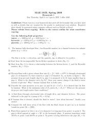
<strong>MAE</strong> <strong>107</strong> <strong>Computational</strong> <strong>Methods</strong> <strong>in</strong> Eng<strong>in</strong>eer<strong>in</strong>g<br />
Spr<strong>in</strong>g 2007<br />
Homework #2 Solutions<br />
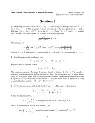
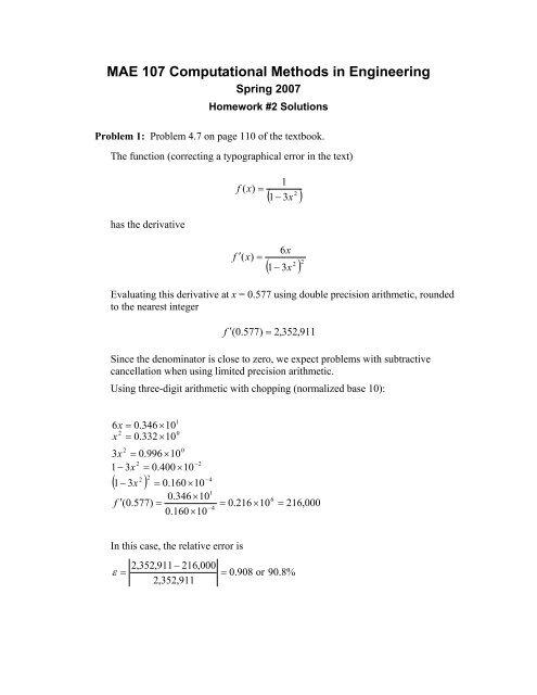
Problem 1: Problem 4.7 on page 110 of the textbook.<br />
The function (correct<strong>in</strong>g a typographical error <strong>in</strong> the text)<br />
has the derivative<br />
f ( x)<br />
=<br />
f ′ ( x)<br />
=<br />
1<br />
2 ( 1−<br />
3x<br />
)<br />
6x<br />
( ) 2 2<br />
1−<br />
3x<br />
Evaluat<strong>in</strong>g this derivative at x = 0.577 us<strong>in</strong>g double precision arithmetic, rounded<br />
to the nearest <strong>in</strong>teger<br />
f ′ ( 0.<br />
577)<br />
=<br />
2,<br />
352,<br />
911<br />
S<strong>in</strong>ce the denom<strong>in</strong>ator is close to zero, we expect problems with subtractive<br />
cancellation when us<strong>in</strong>g limited precision arithmetic.<br />
Us<strong>in</strong>g three-digit arithmetic with chopp<strong>in</strong>g (normalized base 10):<br />
6x<br />
= 0.<br />
346×<br />
10<br />
2<br />
x = 0.<br />
332×<br />
10<br />
2<br />
3x<br />
0<br />
= 0.<br />
996×<br />
10<br />
2<br />
1−<br />
3x<br />
= 0.<br />
400×<br />
10<br />
2 ( 1−<br />
3x<br />
)<br />
f<br />
2<br />
−2<br />
−4<br />
= 0.<br />
160×<br />
10<br />
1<br />
0.<br />
346×<br />
10<br />
′ ( 0.<br />
577)<br />
=<br />
−4<br />
0.<br />
160×<br />
10<br />
1<br />
0<br />
In this case, the relative error is<br />
ε<br />
=<br />
2,<br />
352,<br />
911<br />
−<br />
2,<br />
352,<br />
911<br />
216,<br />
000<br />
6<br />
= 0.<br />
216×<br />
10<br />
=<br />
=<br />
0.<br />
908 or 90.<br />
8%<br />
216,<br />
000
Us<strong>in</strong>g four-digit arithmetic with chopp<strong>in</strong>g (normalized base 10):<br />
6x<br />
= 0.<br />
3462×<br />
10<br />
2<br />
x = 0.<br />
3329×<br />
10<br />
2<br />
3x<br />
0<br />
= 0.<br />
9987 × 10<br />
2<br />
1−<br />
3x<br />
= 0.<br />
1300 × 10<br />
2 ( 1−<br />
3x<br />
)<br />
f<br />
2<br />
−2<br />
−5<br />
= 0.<br />
1690×<br />
10<br />
1<br />
0.<br />
3462×<br />
10<br />
′ ( 0.<br />
577)<br />
=<br />
−4<br />
0.<br />
1690×<br />
10<br />
1<br />
0<br />
7<br />
= 0.<br />
2048×<br />
10<br />
And <strong>in</strong> this case the relative error is<br />
ε =<br />
2,<br />
352,<br />
911<br />
−<br />
2,<br />
352,<br />
911<br />
2,<br />
048,<br />
000<br />
=<br />
=<br />
0.<br />
1296 or 12.<br />
96%<br />
2,<br />
048,<br />
000<br />
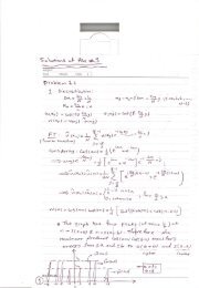
Problem 2: Problem 4.13 on page 110 of the textbook.<br />
Equation (4.11) on page 94 of the textbook is<br />
1<br />
f ( xi<br />
1 ) f ( xi<br />
) f ′ ( xi<br />
)( xi<br />
1 xi<br />
) f ′<br />
+ = +<br />
+ − + ( xi<br />
)( xi+<br />
1 − xi<br />
)<br />
2!<br />
and for the function<br />
we have<br />
2<br />
f ( x)<br />
= ax + bx + c<br />
f ′ ( x)<br />
= 2ax<br />
+ b<br />
.<br />
f ′<br />
( x)<br />
= 2a<br />
Therefore, equation (4.11) becomes<br />
f (<br />
x<br />
i+<br />
1<br />
) = ax<br />
= ax<br />
= ax<br />
2<br />
i<br />
2<br />
i<br />
2<br />
i+<br />
1<br />
2a<br />
2<br />
+ bxi<br />
+ c + ( 2axi<br />
+ b)(<br />
xi+<br />
1 − xi<br />
) + ( xi+<br />
1 − xi<br />
)<br />
2!<br />
+ bx + c + 2ax<br />
x<br />
2<br />
− 2ax<br />
+ bx − bx<br />
2<br />
+ ax − 2ax<br />
x<br />
i<br />
+ bx<br />
i+<br />
1<br />
+ c<br />
i<br />
i+<br />
1<br />
i<br />
i+<br />
1<br />
i<br />
2<br />
i+<br />
1<br />
i<br />
i+<br />
1<br />
+ ax<br />
2<br />
i
<strong>MAE</strong> <strong>107</strong> Spr<strong>in</strong>g 2007<br />
HW 2 Problem 3<br />
Contents<br />
bisect.m<br />
bisect.m<br />
Def<strong>in</strong>e f(x), and plot it<br />
Use bisect.m to compute root of f(x)<br />
Use a smaller <strong>in</strong>terval to see if number of iterations is reduced<br />
type bisect.m<br />
% Function to f<strong>in</strong>d the root of function 'f' near between [x1, x2]<br />
% us<strong>in</strong>g bisection method<br />
function xm = bisect(f, x1, x2)<br />
itmax = 100; % set maximum number of iterations<br />
accuracy = 1e-4; % set required accuracy<br />
prev_xm = NaN; % used for comput<strong>in</strong>g estimated error<br />
disp(spr<strong>in</strong>tf('Desired accuracy = %e\n', accuracy));<br />
for iter = 1:itmax<br />
% calculate midpo<strong>in</strong>t of dcurrent doma<strong>in</strong><br />
xm = (x1 + x2) / 2;<br />
end<br />
disp( spr<strong>in</strong>tf(...<br />
'Iter#=%2d, x-range=(%+6.4f,%+6.4f), xm=%+8.6f, f(xm)=%+8.6e, Estim error=%+6.4e', ...<br />
iter, x1, x2, xm, f(xm), abs(xm - prev_xm)) )<br />
% check if accuracy is acheived<br />
if (abs(f(xm)) < accuracy); break; end<br />
% see if root lies <strong>in</strong> left or right sub-doma<strong>in</strong>?<br />
if (f(x1) * f(xm) > 0) % lies <strong>in</strong> right half<br />
x1 = xm;<br />
else % lies <strong>in</strong> left half<br />
x2 = xm;<br />
end<br />
prev_xm = xm;<br />
disp(spr<strong>in</strong>tf('\nNumber of iterations needed = %d', iter))<br />
end<br />
Def<strong>in</strong>e f(x), and plot it
f = @(x) (exp(x) - 2 + s<strong>in</strong>(2*x)) ;<br />
x = [-3:.01:3];<br />
plot(x, f(x), x, zeros(size(x)));<br />
Use bisect.m to compute root of f(x)<br />
x = bisect(f, -3, +3)<br />
Desired accuracy = 1.000000e-04<br />
Iter#= 1, x-range=(-3.0000,+3.0000), xm=+0.000000, f(xm)=-1.000000e+00, Estim error= NaN<br />
Iter#= 2, x-range=(+0.0000,+3.0000), xm=+1.500000, f(xm)=+2.622809e+00, Estim error=+1.5000e+00<br />
Iter#= 3, x-range=(+0.0000,+1.5000), xm=+0.750000, f(xm)=+1.114495e+00, Estim error=+7.5000e-01<br />
Iter#= 4, x-range=(+0.0000,+0.7500), xm=+0.375000, f(xm)=+1.366302e-01, Estim error=+3.7500e-01<br />
Iter#= 5, x-range=(+0.0000,+0.3750), xm=+0.187500, f(xm)=-4.274972e-01, Estim error=+1.8750e-01<br />
Iter#= 6, x-range=(+0.1875,+0.3750), xm=+0.281250, f(xm)=-1.419126e-01, Estim error=+9.3750e-02<br />
Iter#= 7, x-range=(+0.2812,+0.3750), xm=+0.328125, f(xm)=-1.487416e-03, Estim error=+4.6875e-02<br />
Iter#= 8, x-range=(+0.3281,+0.3750), xm=+0.351562, f(xm)=+6.789124e-02, Estim error=+2.3438e-02<br />
Iter#= 9, x-range=(+0.3281,+0.3516), xm=+0.339844, f(xm)=+3.327809e-02, Estim error=+1.1719e-02<br />
Iter#=10, x-range=(+0.3281,+0.3398), xm=+0.333984, f(xm)=+1.591389e-02, Estim error=+5.8594e-03<br />
Iter#=11, x-range=(+0.3281,+0.3340), xm=+0.331055, f(xm)=+7.217816e-03, Estim error=+2.9297e-03<br />
Iter#=12, x-range=(+0.3281,+0.3311), xm=+0.329590, f(xm)=+2.866336e-03, Estim error=+1.4648e-03
Iter#=13, x-range=(+0.3281,+0.3296), xm=+0.328857, f(xm)=+6.897433e-04, Estim error=+7.3242e-04<br />
Iter#=14, x-range=(+0.3281,+0.3289), xm=+0.328491, f(xm)=-3.987657e-04, Estim error=+3.6621e-04<br />
Iter#=15, x-range=(+0.3285,+0.3289), xm=+0.328674, f(xm)=+1.455065e-04, Estim error=+1.8311e-04<br />
Iter#=16, x-range=(+0.3285,+0.3287), xm=+0.328583, f(xm)=-1.266252e-04, Estim error=+9.1553e-05<br />
Iter#=17, x-range=(+0.3286,+0.3287), xm=+0.328629, f(xm)=+9.441745e-06, Estim error=+4.5776e-05<br />
Number of iterations needed = 17<br />
x =<br />
0.3286<br />
Use a smaller <strong>in</strong>terval to see if number of iterations is reduced<br />
x = bisect(f, -1, +1)<br />
Desired accuracy = 1.000000e-04<br />
Iter#= 1, x-range=(-1.0000,+1.0000), xm=+0.000000, f(xm)=-1.000000e+00, Estim error= NaN<br />
Iter#= 2, x-range=(+0.0000,+1.0000), xm=+0.500000, f(xm)=+4.901923e-01, Estim error=+5.0000e-01<br />
Iter#= 3, x-range=(+0.0000,+0.5000), xm=+0.250000, f(xm)=-2.365490e-01, Estim error=+2.5000e-01<br />
Iter#= 4, x-range=(+0.2500,+0.5000), xm=+0.375000, f(xm)=+1.366302e-01, Estim error=+1.2500e-01<br />
Iter#= 5, x-range=(+0.2500,+0.3750), xm=+0.312500, f(xm)=-4.806479e-02, Estim error=+6.2500e-02<br />
Iter#= 6, x-range=(+0.3125,+0.3750), xm=+0.343750, f(xm)=+4.483311e-02, Estim error=+3.1250e-02<br />
Iter#= 7, x-range=(+0.3125,+0.3438), xm=+0.328125, f(xm)=-1.487416e-03, Estim error=+1.5625e-02<br />
Iter#= 8, x-range=(+0.3281,+0.3438), xm=+0.335938, f(xm)=+2.170613e-02, Estim error=+7.8125e-03<br />
Iter#= 9, x-range=(+0.3281,+0.3359), xm=+0.332031, f(xm)=+1.011753e-02, Estim error=+3.9062e-03<br />
Iter#=10, x-range=(+0.3281,+0.3320), xm=+0.330078, f(xm)=+4.317083e-03, Estim error=+1.9531e-03<br />
Iter#=11, x-range=(+0.3281,+0.3301), xm=+0.329102, f(xm)=+1.415337e-03, Estim error=+9.7656e-04<br />
Iter#=12, x-range=(+0.3281,+0.3291), xm=+0.328613, f(xm)=-3.591366e-05, Estim error=+4.8828e-04<br />
Number of iterations needed = 12<br />
x =<br />
0.3286<br />
Published with MATLAB® 7.3
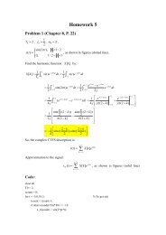
HW 2 Problem 4<br />
Apply<strong>in</strong>g equation (6.6) to f(x)=x n a=0, the n th root of a real number can be calculated as the limit of<br />
x = k1 1<br />
n n−1 x a<br />
k n−1<br />
x<br />
k−1<br />
.<br />
The accuracy at each step can be calculated us<strong>in</strong>g |x k x k1 |. Start<strong>in</strong>g from x(1)=2, k is <strong>in</strong>creased up to the<br />
po<strong>in</strong>t that the accuracy is smaller that 10 6 .<br />
NewtonRaphson.m<br />
%==========================================================================<br />
% Problem 4: This program calculates the nth root of a real positive number<br />
% with accuracy of 10^6 us<strong>in</strong>g NewtonRaphson algorithm.<br />
%==========================================================================<br />
clc;clear;close all;<br />
n=5; % The value of 'n' to calculate the nth root<br />
a=243; % The number which its root is to be determ<strong>in</strong>ed<br />
delta=10; % Residual at each step. It is <strong>in</strong>itialized by a large number...<br />
% ... to start the while loop<br />
x(1)=2; % The <strong>in</strong>itial guess of the root<br />
k=1; % Counter<br />
while (delta>10e6) %checks if the target accuracy is met<br />
end<br />
error(k)=abs(x(k)3); % Absolute error at each time step<br />
k=k+1;<br />
x(k)=(1/n)*((n1)*x(k1)+a/(x(k1)^(n1)));<br />
delta=abs(x(k)x(k1)); % Residuals at each step<br />
error(k)=x(k)3; % Absolute error of the last po<strong>in</strong>t (x(k))<br />
disp('x(1)...x(k):');disp(x); % List<strong>in</strong>g the x(k)s<br />
plot(log(error(1:(k1))),log(error(2:k))); % Plott<strong>in</strong>g ln(E(k+1)) versus ln(E(k))<br />
axis equal; xlabel('ln(E^K)');ylabel('ln(E^{K+1})'); grid on; % Sett<strong>in</strong>g the plot<br />
attributes
Output:<br />
x(1)...x(k):<br />
2.0000 4.6375 3.8151 3.2815 3.0443 3.0013 3.0000 3.0000<br />
Published with MATLAB® 7.1<br />
As we know, tak<strong>in</strong>g the natural logarithm of a quadratic function y=c 1 x 2 +b gives ln(y)=2ln(x)+c 2 where c 1<br />
and c 2 are constants. Thus, plott<strong>in</strong>g the quadratic function <strong>in</strong> the logarithmic scale leads to a straight l<strong>in</strong>e<br />
which makes an angle of tan 1 (2) with the horizontal axis. Based on this discussion, it is clearly seen <strong>in</strong> the<br />
plot above that the Error converges quadratically as expected by equation (6.7).
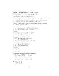
HW 2 Problem 5<br />
Polyroots.m<br />
%==========================================================================<br />
%Problem 5: This program plots the function f(x)=x^5x^43x^3+3x^24x+4 on<br />
%the <strong>in</strong>terval (3,3) and f<strong>in</strong>ds its roots us<strong>in</strong>g the Matlab roots command.<br />
%==========================================================================<br />
clc;clear;close all; % Initializ<strong>in</strong>g the screen, variables and plott<strong>in</strong>g w<strong>in</strong>dows<br />
x=[3:.1:3]; % Def<strong>in</strong><strong>in</strong>g the 'x' vector from 3 to 3 with <strong>in</strong>crements of 0.1<br />
for i=1:length(x) % Calculat<strong>in</strong>g the correspond<strong>in</strong>g 'f' value for each po<strong>in</strong>t of 'x'<br />
end<br />
f(i)=x(i)^5x(i)^43*x(i)^3+3*x(i)^24*x(i)+4;<br />
plot(x,f,'l<strong>in</strong>ewidth',2);grid on; % Plott<strong>in</strong>g the function<br />
ylabel('f(x)');xlabel('x');<br />
root=roots([1 1 3 3 4 4]);hold on; % F<strong>in</strong>d<strong>in</strong>g the roots us<strong>in</strong>g the roots command<br />
display('Roots of the polynom<strong>in</strong>al are :');root %Display<strong>in</strong>g the roots<br />
zer=zeros(1,length(root));<br />
plot(real(root),zer,' ok','MarkerFaceColor','r','MarkerSize',8); %Plott<strong>in</strong>g the real<br />
part of the roots as red circles<br />
%Note: the vector zer is def<strong>in</strong>ed as [0 0... 0] so then the last l<strong>in</strong>e...<br />
%...plots the po<strong>in</strong>ts (root1,0), (root2,0)...(rootn,0)<br />
Output:<br />
Roots of the polynom<strong>in</strong>al are :<br />
root =<br />
2.0000<br />
2.0000<br />
0.0000 + 1.0000i<br />
0.0000 1.0000i<br />
1.0000
Published with MATLAB® 7.1<br />
As the figure shows, the real roots (red circles) obta<strong>in</strong>ed from the roots command co<strong>in</strong>cide with the po<strong>in</strong>ts<br />
that the curve crosses the x axis. However, the red circle located at x=0 does not lay on the curve s<strong>in</strong>ce it is<br />
only represent<strong>in</strong>g the real parts of the two imag<strong>in</strong>ary roots 0+i and 0i.