Section 1.2 Notes - Row Reduction and Echelon Forms
Section 1.2 Notes - Row Reduction and Echelon Forms
Section 1.2 Notes - Row Reduction and Echelon Forms

Create successful ePaper yourself
Turn your PDF publications into a flip-book with our unique Google optimized e-Paper software.
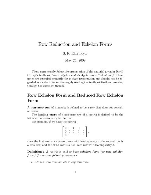
<strong>Row</strong> <strong>Reduction</strong> <strong>and</strong> <strong>Echelon</strong> <strong>Forms</strong><br />
S. F. Ellermeyer<br />
May 24, 2009<br />
These notes closely follow the presentation of the material given in David<br />
C. Lay’s textbook Linear Algebra <strong>and</strong> its Applications (3rd edition). These<br />
notes are intended primarily for in-class presentation <strong>and</strong> should not be regarded<br />
as a substitute for thoroughly reading the textbook itself <strong>and</strong> working<br />
through the exercises therein.<br />
<strong>Row</strong> <strong>Echelon</strong> Form <strong>and</strong> Reduced <strong>Row</strong> <strong>Echelon</strong><br />
Form<br />
A non–zero row of a matrix is de…ned to be a row that does not contain<br />
all zeros.<br />
The leading entry of a non–zero row of a matrix is de…ned to be the<br />
leftmost non–zero entry in the row.<br />
For example, if we have the matrix<br />
2<br />
4<br />
0 0 4 1 0<br />
0 0 0 0 0<br />
0 0 0 0 3<br />
then the …rst row is a non–zero row with leading entry 4, the second row is<br />
a zero row, <strong>and</strong> the third row is a non–zero row with leading entry 3.<br />
De…nition 1 A matrix is said to have echelon form (or row echelon<br />
form) if it has the following properties:<br />
3<br />
5 ,<br />
1. All non–zero rows are above any zero rows.<br />
1
2. Each leading entry of a each non–zero row is in a column to the right<br />
of the leading entry of the row above it.<br />
If a matrix has row echelon form <strong>and</strong> also satis…es the following two<br />
conditions, then the matrix is said to have reduced echelon form (or<br />
reduced row echelon form):<br />
3. The leading entry in each non–zero row is 1.<br />
4. Each leading 1 is the only non–zero entry in its column.<br />
0.1 Quiz<br />
Decide whether or not each of the following matrices has row echelon form.<br />
For each that does have row echelon form, decide whether or not it also has<br />
reduced row echelon form.<br />
1. 2<br />
2. 2<br />
3. 2<br />
4. 2<br />
4<br />
0 0 4 1 0<br />
0 0 0 0 0<br />
0 0 0 0 3<br />
4<br />
4<br />
6<br />
4<br />
1 1 0 1<br />
0 0 1 1<br />
0 0 0 0<br />
1 1 0 0<br />
0 1 1 0<br />
0 0 1 1<br />
1 0 0 0<br />
1 1 0 0<br />
0 1 1 0<br />
0 0 1 1<br />
2<br />
3<br />
5<br />
3<br />
5<br />
3<br />
7<br />
5<br />
3<br />
5
5. 2<br />
6<br />
4<br />
0 1 1 1 1<br />
0 0 2 2 2<br />
0 0 0 0 3<br />
0 0 0 0 0<br />
Given any matrix, we can always perform a sequence of elementary<br />
row operations to arrive at an equivalent matrix that has row echelon form.<br />
In fact, we can always perform a sequence of row operations to arrive at<br />
an equivalent matrix that has reduced row echelon form. For any non–zero<br />
matrix, there are in…nitely many equivalent matrices that have row echelon<br />
form. However, there is only one equivalent matrix that has reduced row<br />
echelon form. (This is proved in Appendix A of the textbook, but we will<br />
not prove it in this course. We will just accept it to be true.)<br />
Theorem 2 (1) Every matrix is equivalent to exactly one matrix that has<br />
reduced row echelon form.<br />
Example 3 Find in…nitely many di¤erent matrices that have row echelon<br />
form <strong>and</strong> that are equivalent to the matrix<br />
2<br />
0 0 4 1<br />
3<br />
0<br />
4 0 0 0 0 0 5 .<br />
0 0 0 0 3<br />
Then …nd the unique matrix that has reduced row echelon form <strong>and</strong> that is<br />
equivalent to this matrix.<br />
Solution 4 By performing an interchange operation, we obtain<br />
2<br />
0 0 4 1<br />
3<br />
0<br />
2<br />
0 0 4 1<br />
3<br />
0<br />
4 0 0 0 0 0 5 4 0 0 0 0 3 5 .<br />
0 0 0 0 3 0 0 0 0 0<br />
The matrix on the right is equivalent to the matrix on the left <strong>and</strong> has row<br />
echelon form. If we like, we can now scale the top row by 3 to obtain the<br />
matrix 2<br />
0 0 12 3<br />
3<br />
0<br />
4 0 0 0 0 3 5<br />
0 0 0 0 0<br />
3<br />
3<br />
7<br />
5
which also has row echelon form <strong>and</strong> which is also equivalent to the original<br />
matrix.<br />
Clearly, we can obtain an in…nite number of such matrices by continuing<br />
to scale the …rst or second rows by whatever non–zero number we like.<br />
To …nd the unique reduced row echelon matrix that is equivalent to the<br />
original matrix, we continue the row operations started above as follows:<br />
2<br />
4<br />
0 0 4 1 0<br />
0 0 0 0 0<br />
0 0 0 0 3<br />
3<br />
5<br />
2<br />
4<br />
0 0 4 1 0<br />
0 0 0 0 3<br />
0 0 0 0 0<br />
3<br />
5<br />
2<br />
4<br />
0 0 1 1<br />
4 0<br />
0 0 0 0 3<br />
0 0 0 0 0<br />
The matrix on the far right has reduced row echelon form <strong>and</strong> is equivalent<br />
to the original matrix. No other such reduced echelon matrix can be found.<br />
(This is guaranteed by Theorem 1.)<br />
Notation 5 For any matrix A, we will use the notation rref (A) to denote<br />
the unique matrix having reduced row echelon form <strong>and</strong> equivalent to A. (This<br />
notation is not used in the textbook we are using but it is done in many other<br />
books.)<br />
then<br />
For example, if<br />
2<br />
A = 4<br />
rref (A) = 4<br />
0 0 4 1 0<br />
0 0 0 0 0<br />
0 0 0 0 3<br />
2<br />
3<br />
5 ,<br />
0 0 1 1<br />
4 0<br />
0 0 0 0 1<br />
0 0 0 0 0<br />
1 Pivot Positions <strong>and</strong> Pivot Columns<br />
De…nition 6 A pivot position in a matrix, A, is a location in A that<br />
corresponds to a leading 1 in rref (A). A pivot column in A is a column<br />
of A that contains a pivot position.<br />
For example, look at the matrices A <strong>and</strong> rref (A) in the example done<br />
above. The pivot positions in A are the positions indicated below:<br />
2<br />
0<br />
6<br />
A = 4 0<br />
0<br />
0<br />
4<br />
pivot position<br />
0<br />
1<br />
0<br />
3<br />
0<br />
7<br />
0 5<br />
pivot position<br />
0 0 0 0 3<br />
4<br />
3<br />
5<br />
3<br />
5<br />
2<br />
4<br />
0 0 1 1<br />
4 0<br />
0 0 0 0 1<br />
0 0 0 0 0<br />
3<br />
5 .
<strong>and</strong> the pivot columns of A are the third <strong>and</strong> …fth columns. Note that we<br />
can only tell what the pivot positions <strong>and</strong> pivot columns of a matrix, A, are<br />
after we have found rref (A).<br />
Example 7 Find the pivot positions <strong>and</strong> pivot columns of the matrix<br />
2<br />
6<br />
A = 6<br />
4<br />
0<br />
1<br />
2<br />
3<br />
2<br />
3<br />
6<br />
1<br />
0<br />
4<br />
3<br />
3<br />
3<br />
9<br />
1 7<br />
1 5<br />
1 4 5 9 7<br />
.<br />
Solution 8 Since<br />
rref (A) =<br />
2<br />
6<br />
4<br />
1 0 3 0 5<br />
0 1 2 0 3<br />
0 0 0 1 0<br />
0 0 0 0 0<br />
3<br />
7<br />
5 ,<br />
we see that the pivot positions of A are as indicated below:<br />
2<br />
0<br />
pivot position<br />
6 1<br />
A = 6<br />
4 2<br />
3<br />
2<br />
pivot position<br />
3<br />
6<br />
1<br />
0<br />
4<br />
3<br />
3<br />
pivot position<br />
3<br />
9<br />
7<br />
1 7<br />
1 5<br />
1 4 5 9 7<br />
.<br />
The pivot columns of A are the …rst, second, <strong>and</strong> fourth columns.<br />
2 The <strong>Row</strong> <strong>Reduction</strong> Algorithm<br />
Here is an algorithm that always works for …nding rref (A) for any matrix<br />
A.<br />
1. Begin with the leftmost non–zero column. This is a pivot column. The<br />
pivot position is at the top.<br />
2. If the top entry in this column is 0, then interchange the top row with<br />
some other row that has a non–zero entry as its …rst entry. Then scale<br />
the top row to make the leading entry be a 1.<br />
5
3. Use replacement operations to create zeros in every position in this<br />
column below the pivot position.<br />
4. Cover (or ignore) the row containing the pivot position <strong>and</strong> cover (or<br />
ignore) any rows above it. Repeat steps 1, 2, <strong>and</strong> 3 for the submatrix<br />
that remains. Repeat the process until there is no non–zero column in<br />
the submatrix that remains.<br />
5. Beginning with the rightmost pivot position <strong>and</strong> working upward <strong>and</strong><br />
to the left, create zeros above each pivot position by using replacement<br />
operations.<br />
Example 9 For the matrix<br />
2<br />
A = 4<br />
0 1 1 0<br />
2 0 5 5<br />
4 4 5 0<br />
use the reduction algorithm to …nd rref (A).<br />
Answer:<br />
2<br />
rref (A) = 4<br />
3<br />
5 ;<br />
1 0 0 45<br />
2<br />
0 1 0 10<br />
0 0 1 10<br />
3 Solutions of Linear Systems<br />
It is easy to …nd the solution set of a linear system whose augmented matrix<br />
has reduced row echelon form. Also, if [A j b] is the augmented matrix of a<br />
system, then the solution set of this system is the same as the solution set<br />
of the system whose augmented matrix is rref ([A j b]) (since the matrices<br />
[A j b] <strong>and</strong> rref ([A j b]) are equivalent). Thus, …nding rref ([A j b]) allows<br />
us to solve any given linear system. This is illustrated in the three examples<br />
that follow. In the …rst example, it turns out that the system is inconsistent.<br />
In the second example, the system has in…nitely many solutions. In the third<br />
example, the system has a unique solution.<br />
6<br />
3<br />
5 .
Example 10 Find the solution set of the linear system<br />
3x1 4x2 = 9<br />
2x1 + 4x2 x3 = 0<br />
10x1 2x3 = 4.<br />
Solution 11 The augmented matrix of this system is<br />
2<br />
3 4 0 9<br />
3<br />
[A j b] = 4 2 4 1 0 5<br />
10 0 2 4<br />
<strong>and</strong><br />
2<br />
1 1 0 5<br />
rref ([A j b]) = 4<br />
0<br />
0 1 3<br />
20 0<br />
0 0 0 1<br />
Since rref ([A j b]) is the augmented matrix of the linear system<br />
x2<br />
x1<br />
1<br />
5 x3 = 0<br />
3<br />
20 x3 = 0<br />
0 = 1<br />
which obviously has no solution (because of the equation 0 = 1), we conclude<br />
that the original system that was given is also inconsistent. (Its solution set<br />
is the empty set.)<br />
As an important remark, note that what causes this system to be inconsistent<br />
is the fact that the last column of its augmented matrix is a pivot<br />
column.<br />
Example 12 Find the solution set of the linear system<br />
3x1 4x2 = 9<br />
2x1 + 4x2 x3 = 0<br />
10x1 2x3 = 18.<br />
Solution 13 The augmented matrix of this system is<br />
2<br />
3 4 0 9<br />
3<br />
[A j b] = 4 2 4 1 0 5<br />
10 0 2 18<br />
7<br />
3<br />
5 .
<strong>and</strong><br />
2<br />
1 9<br />
1 0 5 5<br />
rref ([A j b]) = 4<br />
3 0 1 20<br />
0 0 0 0<br />
The matrix rref ([A j b]) is the augmented matrix for the linear system<br />
x2<br />
x1<br />
1<br />
5 x3 = 9<br />
5<br />
3<br />
20 x3<br />
9<br />
=<br />
10<br />
0 = 0<br />
This system is consistent <strong>and</strong> has in…nitely many solutions. To obtain a<br />
solution, we can let x3 be any number that we like <strong>and</strong> then let<br />
<strong>and</strong> then let<br />
x2 = 9 3<br />
+<br />
10 20 x3,<br />
x1 = 9<br />
5<br />
+ 1<br />
5 x3.<br />
Since x3 can be any number that we like (for which reason we say that x3 is<br />
a free variable), we see that the system under consideration has in…nitely<br />
many solutions. As an example of a particular solution, suppose we let x3 =<br />
10. Then<br />
<strong>and</strong><br />
x2 = 9 3 3<br />
+ (10) =<br />
10 20 5<br />
x1 = 9 1 19<br />
+ (10) =<br />
5 5 5 .<br />
19 3<br />
Thus, the ordered triple ; ; 10 is a solution of the original system. Let<br />
5 5<br />
us check:<br />
2<br />
3<br />
19<br />
5<br />
10<br />
19<br />
5<br />
+ 4<br />
19<br />
5<br />
3<br />
5<br />
4<br />
8<br />
3<br />
5<br />
= 9<br />
10 = 0<br />
9<br />
10<br />
2 (10) = 18.<br />
3<br />
5 .
As an important remark, note that was causes this system to have in…nitely<br />
many solutions is the fact the last column of its augmented matrix is<br />
not a pivot column (thus making the system consistent) together with the fact<br />
that not every column of its coe¢ cient matrix is a pivot column (allowing the<br />
system to have free variables).<br />
Example 14 Find the solution set of the linear system<br />
3x1 4x2 = 9<br />
2x1 + 4x2 x3 = 0<br />
x1 x3 = 0.<br />
Solution 15 The augmented matrix of this system is<br />
2<br />
3 4 0<br />
3<br />
9<br />
[A j b] = 4 2 4 1 0 5<br />
1 0 1 0<br />
<strong>and</strong><br />
2<br />
rref ([A j b]) = 4<br />
9 1 0 0 4<br />
9<br />
0 1 0 16<br />
9 0 0 1 4<br />
Since rref ([A j b]) is the augmented matrix of the linear system<br />
x1 = 9<br />
4<br />
x2 =<br />
x3 = 9<br />
4 ,<br />
9<br />
we conclude that the only solution of the original system is 4 ; 9 9 ; 16 4 .<br />
Note that the reason that this system has a unique solution is that its<br />
last column is not a pivot column (meaning that the system is consistent)<br />
together with the fact that every column of its coe¢ cient matrix is a pivot<br />
column (meaning that the system has no free variables).<br />
9<br />
9<br />
16<br />
3<br />
5 .
4 Answering the “Existence <strong>and</strong> Uniqueness”<br />
Questions<br />
Suppose that we have a linear system whose coe¢ cient matrix is A <strong>and</strong><br />
whose augmented matrix is [A j b]. Then [A j b] is the same as A except<br />
for the fact that [A j b] has an extra column on the right. Because of the<br />
way that elementary row operations work, the matrix rref ([A j b]) is also<br />
the same as rref (A) except, once again, for the fact that rref ([A j b]) has<br />
an extra column on the right. Inspired by the preceding three examples, we<br />
arrive at the following criteria for answering the questions:<br />
1. Does our system have a solution? (Existence)<br />
2. If so, then does it have just one solution or in…nitely many? (Uniqueness)<br />
Theorem 16 (2) For a linear system with coe¢ cient matrix A <strong>and</strong> augmented<br />
matrix [A j b] :<br />
1. The system is consistent if <strong>and</strong> only if the last column of [A j b] is not<br />
a pivot column.<br />
2. If the system is consistent, then the system has a unique solution if <strong>and</strong><br />
only if every column of A is a pivot column.<br />
Example 17 Answer the existence <strong>and</strong> uniqueness questions for the system<br />
x1 + 2x2 5x3 6x4 = 5<br />
x2 6x3 3x4 = 2<br />
x4 5x5 = 5.<br />
Solution 18 The coe¢ cient matrix for this system is<br />
2<br />
1 2 5 6 0<br />
3<br />
A = 4 0 1 6 3 0 5<br />
0 0 0 1 5<br />
10
<strong>and</strong> the augmented matrix is<br />
2<br />
Also,<br />
[A j b] = 4<br />
rref ([A j b]) = 4<br />
1 2 5 6 0 5<br />
0 1 6 3 0 2<br />
0 0 0 1 5 5<br />
2<br />
3<br />
5 .<br />
1 0 7 0 0 9<br />
0 1 6 0 15 13<br />
0 0 0 1 5 5<br />
from which we can immediately conclude that the system is consistent (because<br />
the last column of [A j b] is not a pivot column).<br />
In addition,<br />
2<br />
rref (A) = 4<br />
1 0 7 0 0<br />
0 1 6 0 15<br />
0 0 0 1 5<br />
from which we conclude that the system has in…nitely many solutions<br />
(rather than a unique solution) because not every column of A is a pivot<br />
column.<br />
As an important remark, we note that it is not necessary to compute<br />
rref (A) separately once rref ([A j b]) has been computed. This is because<br />
rref (A) will always be the same as rref ([A j b]) with the last column deleted.<br />
Example 19 For the system given in the above example (which was found to<br />
have in…nitely many solutions), give a parametric description of its solution<br />
set.<br />
Solution 20 Looking at the matrix rref ([A j b]) in the above example, we<br />
see that the system in that example is equivalent to the system<br />
x1 + 7x3 = 9<br />
x2 6x3 15x5 = 13<br />
x4 5x5 = 5.<br />
The free variables for this system (corresponding to the non–pivot columns<br />
in rref (A)) are x3 <strong>and</strong> x5. The general solution of the system (described in<br />
11<br />
3<br />
5 ,<br />
3<br />
5
parametric form) is<br />
x1 = 9 7x3<br />
x2 = 13 + 6x3 + 15x5<br />
x3 = free<br />
x4 = 5 + 5x5<br />
x5 = free.<br />
12