A very basic tutorial for performing linear mixed

More documents

Recommendations

Info

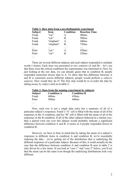
Table 1: Raw data from a psycholinguistic experiment Subject Item Condition Reaction Time Frank “car” A 400ms Frank “car” B 500ms Frank “elephant” A 440ms Frank “elephant” B 750ms … … … … Peter “car” A 430ms Peter “car” B 520ms … There are several different subjects and each subject responded to multiple words (=items). Each item was presented in two contexts (A and B) – let’s say that these were the critical conditions the experimenter was interested in. Now, by just looking at the raw data, we can already guess that in condition B, people responded somewhat slower than in A. To show that this difference between A and B is consistent across different subjects, people would perform a subjects analysis. How would they do it? The first step would be to re-order the data by taking means by subject such as in table 2: Table 2: Data from the naming experiment by subjects Subject Condition A Condition B Frank 400ms 450ms Peter 500ms 600ms … Now, each row is not a single data entry but a summary of all of a particular subject’s responses. Frank’s “A” cell is filled with the mean of all of his responses in the A condition, and his “B” cell is filled with the mean of all of his responses in the B condition. If all of the other subjects behaved in a similar way, then a paired t-test run over this dataset would probably indicate a significant difference between condition A and B: it seems as if people responded slower in condition B. However, we have to bear in mind that by taking the mean of a subject’s responses to different items in condition A and condition B, we’re essentially reducing the data – we’re getting rid of the distribution that is underlying the different responses of a particular subject. Because of this, it could actually be the case that the difference between condition A and condition B seen in table 2 is only driven by a few items. If you look at “case 1” and “case 2” below, you’ll see that the mean can be the same even though the underlying distributions look very different. 2
Case 1 400 400 400 400 mean: 400 Case 2 200 200 200 1000 mean: 400 Because both “case 1” and “case 2” are likely possibilities, and because table 2 does not allow us to see with which of these cases we’re dealing, we need to construct a different table, one where we take the means by items: Table 3: Data from our experiment with means by items Item Condition A Condition B “car” 220ms 210ms “elephant” 230ms 1000ms “pig” 190ms 200ms “truck” 200ms 200ms ... Here, we’re essentially ignoring the subject information. And in this hypothetical example, we can indeed see that the difference between A and B that was observed in the subjects analysis was due to just a few items. It seems to be the case that the one extreme value in condition B, the 1000ms response to the word “elephant” influenced the pattern that we observed by looking at the data by subjects. If we were to run a paired t-test on this dataset, it would probably not indicate a significant difference… This example highlights that looking at data by subjects or by items can lead to vastly different conclusions. One of Herbert Clark’s main contributions was to highlight the importance of the items analysis, and similar arguments have been made in other fields than just psycholinguistics. Now, it’s time to introduce some new terminology that will later help us with the linear mixed effects models. When we did the subjects analysis, we took “Subjects” as a random effect. Basically this means that we expect random variation from each subject, because after all, everybody will have slightly different reaction times based on a various reasons that we can’t control in our experiments (e.g. some people are just slower than others, some subjects might be stoned when appearing to your experiment etc.). When we did the items analysis, we took “Items” as a random effect. Each word has a range of different features that might affect reaction times (frequency, word class, word length etc.), some of which we won’t be able to control in our experiment. From the perspective of the experiment, both subjects and items will influence the reaction times in a way that is – at least to some extent – unpredictable or “random”. Things that induce some 3
Page 1: A very basic tutorial for performin
Page 5 and 6: occurrence of a yes response (categ
Page 7 and 8: The reason why the first command in
Page 9 and 10: politeness.model.p = pvals.fnc(poli
Page 11 and 12: politeness.model = lmer(frequency ~
Page 13 and 14: that the model predicts, and a “r
Page 15 and 16: Then, we perform a so-called likeli
Page 17: Clark, H. H. (1973). The language-a

A very basic tutorial for performing linear mixed

Create successful ePaper yourself

Delete template?

Save as template?