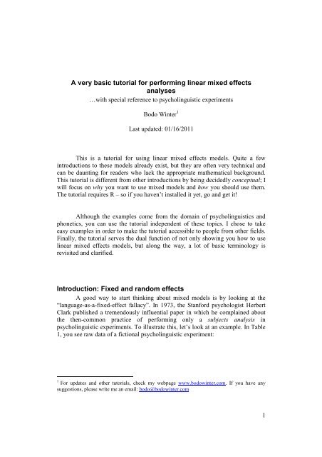
A very basic tutorial for performing linear mixed

A very basic tutorial for performing linear mixed effects
analyses
…with special reference to psycholinguistic experiments
Bodo Winter 1
Last updated: 01/16/2011
This is a tutorial for using linear mixed effects models. Quite a few
introductions to these models already exist, but they are often very technical and
can be daunting for readers who lack the appropriate mathematical background.
This tutorial is different from other introductions by being decidedly conceptual; I
will focus on why you want to use mixed models and how you should use them.
The tutorial requires R – so if you haven’t installed it yet, go and get it!
Although the examples come from the domain of psycholinguistics and
phonetics, you can use the tutorial independent of these topics. I chose to take
easy examples in order to make the tutorial accessible to people from other fields.
Finally, the tutorial serves the dual function of not only showing you how to use
linear mixed effects models, but along the way, a lot of basic terminology is
revisited and clarified.
Introduction: Fixed and random effects
A good way to start thinking about mixed models is by looking at the
“language-as-a-fixed-effect fallacy”. In 1973, the Stanford psychologist Herbert
Clark published a tremendously influential paper in which he complained about
the then-common practice of performing only a subjects analysis in
psycholinguistic experiments. To illustrate this, let’s look at an example. In Table
1, you see raw data of a fictional psycholinguistic experiment:
1 For updates and other tutorials, check my webpage www.bodowinter.com. If you have any
suggestions, please write me an email: bodo@bodowinter.com
1

Table 1: Raw data from a psycholinguistic experiment
Subject Item Condition Reaction Time
Frank “car” A 400ms
Frank “car” B 500ms
Frank “elephant” A 440ms
Frank “elephant” B 750ms
… … … …
Peter “car” A 430ms
Peter “car” B 520ms
…
There are several different subjects and each subject responded to multiple
words (=items). Each item was presented in two contexts (A and B) – let’s say
that these were the critical conditions the experimenter was interested in. Now, by
just looking at the raw data, we can already guess that in condition B, people
responded somewhat slower than in A. To show that this difference between A
and B is consistent across different subjects, people would perform a subjects
analysis. How would they do it? The first step would be to re-order the data by
taking means by subject such as in table 2:
Table 2: Data from the naming experiment by subjects
Subject Condition A Condition B
Frank 400ms 450ms
Peter 500ms 600ms
…
Now, each row is not a single data entry but a summary of all of a
particular subject’s responses. Frank’s “A” cell is filled with the mean of all of his
responses in the A condition, and his “B” cell is filled with the mean of all of his
responses in the B condition. If all of the other subjects behaved in a similar way,
then a paired t-test run over this dataset would probably indicate a significant
difference between condition A and B: it seems as if people responded slower in
condition B.
However, we have to bear in mind that by taking the mean of a subject’s
responses to different items in condition A and condition B, we’re essentially
reducing the data – we’re getting rid of the distribution that is underlying the
different responses of a particular subject. Because of this, it could actually be the
case that the difference between condition A and condition B seen in table 2 is
only driven by a few items. If you look at “case 1” and “case 2” below, you’ll see
that the mean can be the same even though the underlying distributions look very
different.
2

Case 1
400 400 400 400 mean: 400
Case 2
200 200 200 1000 mean: 400
Because both “case 1” and “case 2” are likely possibilities, and because
table 2 does not allow us to see with which of these cases we’re dealing, we need
to construct a different table, one where we take the means by items:
Table 3: Data from our experiment with means by items
Item Condition A Condition B
“car” 220ms 210ms
“elephant” 230ms 1000ms
“pig” 190ms 200ms
“truck” 200ms 200ms
...
Here, we’re essentially ignoring the subject information. And in this
hypothetical example, we can indeed see that the difference between A and B that
was observed in the subjects analysis was due to just a few items. It seems to be
the case that the one extreme value in condition B, the 1000ms response to the
word “elephant” influenced the pattern that we observed by looking at the data by
subjects. If we were to run a paired t-test on this dataset, it would probably not
indicate a significant difference…
This example highlights that looking at data by subjects or by items can
lead to vastly different conclusions. One of Herbert Clark’s main contributions
was to highlight the importance of the items analysis, and similar arguments have
been made in other fields than just psycholinguistics.
Now, it’s time to introduce some new terminology that will later help us
with the linear mixed effects models. When we did the subjects analysis, we took
“Subjects” as a random effect. Basically this means that we expect random
variation from each subject, because after all, everybody will have slightly
different reaction times based on a various reasons that we can’t control in our
experiments (e.g. some people are just slower than others, some subjects might be
stoned when appearing to your experiment etc.). When we did the items analysis,
we took “Items” as a random effect. Each word has a range of different features
that might affect reaction times (frequency, word class, word length etc.), some of
which we won’t be able to control in our experiment. From the perspective of the
experiment, both subjects and items will influence the reaction times in a way that
is – at least to some extent – unpredictable or “random”. Things that induce some
3

amount of random variation into your data, statisticians like to call “random
effects”.
The counter-term to “random effect” is “fixed effect”. Things that you
control in your experiment, where you predict or expect a certain systematic
difference between conditions are called “fixed effects” or “factors”. Fixed effects
can be categorical and discontinuous (e.g. male vs. female) or numerical and
continuous (e.g. articulation rate).
So, before we go on to the actual linear mixed effects models, let’s just see
what happened in response to Clark’s paper. In the end, his critique led to the
requirement that whenever you present multiple items to each subject, you have to
perform a subjects analysis and an items analysis. Therefore, you’ll find in almost
all psycholinguistic publications that two test statistics are reported, e.g. F1 and F2
(ANOVA) or t1 and t2 (t-test). A result could read something like this:
Or simply:
“We obtained a significant effect of Frequency for both subjects
(F1(32)=16.43, p=0.0043) and items (F2(16)=5.78, p=0.0032).”
“We obtained a significant effect of Frequency (F1(32)=16.43, p=0.0043;
F2(16)=5.78, p=0.0032).”
The subscript 1 stands for the subjects analysis, the subscript 2 stands for
the items analysis. Usually, it is required that both test statistics are significant
(see Raaijmakers et al. 1999 for a critique of this standard). If, for example, the
subjects analysis reaches an accepted significance level such as α=0.05 but the
items analysis does not, then this might indicate that only a few individual items
lead to the effect observed in the subjects analysis. In other words, you could say
the effect does not generalize over items.
Now, mixed models improve upon the common practice of doing separate
tests for subjects and items by allowing you to combine random effects. In essence,
this means that you can generalize across both subjects and items with a single
model. So, you don’t need to do two separate statistical tests anymore. Mixed
models have several other advantages:
1. You can include categorical and numerical predictor variables in your
experiment. For example, you could test the combined effect of the
fixed effects Articulation Rate (numerical/continuous) and Gender
(categorical/discontinuous) on a set of measures you’ve done.
2. You can use mixed models for both categorical/discontinuous and
numerical/continuous data. For example, you can predict the
4

occurrence of a yes response (categorical/discontinuous), as well as
reaction times and other numerical/continuous dependent measures.
Sounds cool? So let’s do it! In the following, I present to you how to use
mixed models in R. For this, you need to have R installed.
Linear mixed effects models in R
For a start, we need to install the R packages lme4 (Bates & Maechler,
2009) and languageR (Baayen, 2009; cf. Baayen, 2008). While being connected
to the internet, open R and type in:
install.packages( )
Select a server close to you and then choose the packages lme4 and
languageR. In order to be able to use the packages, you have to load them into the
R environment with the following command:
library(lme4);library(languageR)
Now, you have several new commands available to you, among them
lmer( ), which is the basic command for performing mixed effects models
provided by the lme4 package, and pvals.fnc( ), which is the a command for
getting p-values from mixed models provided by the languageR package.
To go on, we need some data. For this tutorial, I’m using a dataset that is
available on: http://www.bodowinter.com/tutorial/politeness_data.csv
This is a shortened version of a dataset that was used for Grawunder &
Winter (2010) and Winter & Grawunder (submitted). Put the data into your /bin/
folder where you’ve installed R. Then, load the data into R:
politeness

With this data (which is from Korean speakers, by the way), we were
interested in the phonetic difference between polite and informal speech. Whether
a given response was in the polite or the informal condition is given in the column
“attitude”. The dependent measure in this example is voice pitch given in the
column called “frequency”. The units of frequency are given in Hertz (Hz). One
last thing: you need to know that we took repeated measures from each subject,
meaning that each subject was presented multiple context scenarios in the polite
and informal condition. The number of the context scenario is given in the column
“scenario”.
Because the three most important rules of statistics are “Draw a picture,
draw a picture, draw a picture” (Michael Starbird), let’s make a boxplot before we
start constructing mixed models. In fact, before you do any inferential statistics
you should always explore the data extensively.
boxplot(frequency ~ attitude, data=politeness)
100 150 200 250 300
inf pol
It looks like the voice pitch was lower in the polite condition. This is
important because – before we do any statistical tests – we can formulate the
expectation that the mixed model will show (if anything) a lowering of voice
pitch in the polite condition. Let’s also look at the medians of the two conditions.
median(politeness[which(politeness$attitude=="pol"
),]$frequency, na.rm=T)
median(politeness[which(politeness$attitude=="inf"
),]$frequency)
6

The reason why the first command includes the additional argument
na.rm=T is that R is reluctant to give you a median value if there is a missing
value, and as we pointed out before, there is a missing value in the polite
condition in line 263.
The median( ) commands give you the median 185.5 Hz for the polite
condition and the median of 209.05 Hz for the informal condition. So, there seems
to be a difference of about 23.55 Hz. Now, let’s see whether this difference
between the polite and the informal condition depends on whether the speaker is
male or female; let’s add the factor Gender to our boxplot.
boxplot(frequency ~ attitude*gender,
data=politeness)
100 150 200 250 300
inf.F pol.F inf.M pol.M
What do we see? Well, the results for females and males do not look
qualitatively different from each other: in both cases the voice pitch is lower in
the polite condition. So, just by looking at this boxplot, there does not seem to be
an interaction between the factors Politeness and Gender. Again, this is important
for formulating expectations with respect to your mixed effects analysis. It cannot
be emphasized enough how important it is to look at the data extensively before
you start doing an analysis.
Now, let’s start building a model. By doing so, we’re leaving the domain
of descriptive statistics (summarizing and displaying data) and we enter the
domain of inferential statistics (testing whether the differences that we saw with
descriptive statistics are chance results or not). By doing inferential statistics such
7

as linear mixed effects models, we want to know whether the difference in voice
pitch between the polite and the informal condition are due to chance…
We will now use the function lmer( ). This command takes as its first
argument a formula very similar to the one we used in the boxplot( ) command.
When we created the boxplots, we displayed frequency values with respect to the
factor attitude, now we want to predict frequency values with respect the factor
attitude. So, to the left of the tilde we put the thing that we seek to explain or
predict, the dependent measure. To the right of the tilde, we put the fixed effect
that we use to predict pitch, the predictor variable or the fixed effect. In the
example below, there’s no random effect and if you type in the command, you
will retrieve an error:
lmer(frequency ~ attitude, data=politeness)
The reason for this error is that the linear mixed effect model needs a
random effect. So we need to introduce a random effect, and the way this is done
is a little bit cryptic:
(1|subject)
… means “Subject as a random effect” and likewise
(1|item)
… means “Item as a random effect”.
In our example, the items are scenarios. Therefore, the command that we
need to use is:
politeness.model = lmer(frequency ~ attitude +
(1|subject) + (1|scenario), data=politeness)
With this command, we created a model that predicted frequency based on
the fixed effect “attitude” and the random effects “subject” and “scenario”, and
we saved this model in the object politeness.model. Type in politeness.model and
see what it gives you. Among other things, you see a t-value for the fixed effect
which is -2.547. t-values approaching 2 or -2 usually reach significance if there’s
enough data. Usually, you would now look on a table (or use your computer) to
find the p-value associated with that specific t-value. However, that’s not possible
in this case because you don’t know the degrees of freedom. So, how can we
assess the statistical significance of the results? Harald Baayen developed a
function pvals.fnc( ) that gives you p-values based on Markov-chain Monte Carlo
sampling, so called MCMC-estimated p-values.
8

politeness.model.p = pvals.fnc(politeness.model)
By typing in the above expression, you calculate the p-values based on the
model that is saved in the object politeness.model. The p-values are saved in the
object politeness.model.p. Type in the name of this object to see the following
results:
Right now, let’s only look at the p-values for the fixed effects and not at
the random effects (later on, you can access only the fixed effects by typing in
politeness.model.p$fixed). So, what do we see? There are two rows, one is called
“(Intercept)” and one is called “attitudepol”. Then, there are several columns of
which the two most important are “Estimate” and “pMCMC”. Let’s look at
“attitudepol” first. “Attitudepol” is an abbreviation for “the polite level of the
factor Attitude” (as opposed to the level informal). In the “Estimate” column, you
see -19.19, which is actually a numerical value of our measurement (frequency in
Hertz). So, the table says that for the polite condition (as opposed to the informal
condition), you need to decrease frequency by 19.19 Hz. In the pMCMC, you see
the value 0.0460. This is the MCMC-estimated p-value. So, by a standard α-level
of 0.05, this result is significant … which means that it is relatively unlikely due
to chance.
Now, the row “(Intercept”) indicates your “starting point”. If you think
back to high school math, the intercept refers to the value where a line meets the
y-axis of a plot:
y-intercept
9

The model takes the mean of all data points as the value that it would
estimate “to start with”. Then, all the other effects are predicted on the basis of
this starting value, e.g. to arrive at a good estimate of pitch in the polite condition,
you have to decrease the mean by 19 Hz.
In our example, the intercept has the estimate 192.05 Hz. This is the mean
of all frequencies taken together, including both males and females. Since males
have relatively low Hertz values and females relatively high Hertz values, you
end up with a mean that is between the two. This is a classic example of a
bimodal distribution, a distribution that has two modes (=the most frequent value).
To see this, compare the mean of the complete dataset:
mean(politeness$frequency, na.rm=T)
To the mean of the mean of the male and female subsets:
mean(politeness[which(politeness$gender ==
"F"),]$frequency)
mean(politeness[which(politeness$gender ==
"M"),]$frequency, na.rm=T)
In some way, an intercept of 192.05 Hz does not make much sense. This is
similar to the classic example of a farm with a dozen hens and a dozen cows ….
where, if you were to take the arithmetic mean number of legs on the farm, you
would make the meaningless statement that the animals of the farm have on
average three legs. So, we should inform our model that multiple genders are
present in our data and that therefore, vast differences in voice pitch are to be
expected. Currently, our model does not account for Gender.
Should Gender be a fixed or a random effect? Some people might be
tempted to put “gender” as a random effect because they want to “generalize
over” genders… however, this is not a good idea because the variation in
frequencies that you expect to come from male and female participants is not
“random” but in fact quite systematic and predictable. So we want to add gender
as a fixed effect, as if we were doing a controlled experiment with four
conditions: male|polite, male|informal, female|polite and female|informal. What
we’re interested in is not only the effect of gender on frequencies in general, but
also on the effect of gender on frequencies with respect to politeness. We can test
this by adding gender to the model and putting a * between the fixed effects
gender and politeness. This * says to the model that we’re not only interested in
the fixed effect gender and the fixed effect politeness, but also in the interaction
of these two factors.
10

politeness.model = lmer(frequency ~
attitude*gender + (1|subject) + (1|scenario),
data=politeness)
politeness.model.p = pvals.fnc(politeness.model)
Note that you’ve overwritten the model and the p-value output object of
the first mixed model analysis that we performed. Check the results by typing
politeness.model.p$fixed.
What do we see? The intercept is 256 Hz (the mean frequency of the
female participants…). So the model takes the voice pitch of females as the
starting value. Why does it take the females and not the males? If you type in the
following…
levels(politeness$gender)
… you see that “F” for female is listed before “M”. The model simply
takes the first level of a factor as the intercept.
The fact that the intercept reaches significance (p < 0.0001) simply means
that the intercept is significantly different from 0. It usually does not matter much
if the intercept is significant or not.
Now, to accurately predict the frequency of the polite condition as
opposed to the frequency of the informal condition, you need to lower the
frequencies by 29.27 Hz. This result is unlikely due to chance as indicated by the
low p-value (p=0.0122). Then, with respect to gender, you need to lower
frequencies by 127.94 Hz for males. As we would expect, this difference is
unlikely due to chance as well (p=0.0008). The “attitudepol” and “genderM” rows
indicate so-called main effects (you only consider the effect of a single factor).
The last column “attitudepol:genderM” indicates an interaction effect because it
includes two factors. Whenever you include an interaction effect into your model
with *, the model will automatically compute the corresponding main effects as
well.
The estimate of the interaction effect is a little bit difficult to read: “for the
polite condition you need to go up by 20.38 Hz for males”. Interaction effects are
often difficult to read and in order to see in which direction the effect is going,
11

you usually need to make extra graphs and tests rather than looking at the
estimates output of the mixed models. Crucially however, the mixed model
confirms an expectation that we had by looking at boxplot 2: The interaction
between attitude and gender is not significant (p=0.1916), meaning that whatever
interaction there is in the dataset right now is likely due to chance. We expected
this result based on boxplot 2 where we didn’t see a big difference of polite vs.
informal for males and females.
However, what would happen if there were a significant interaction effect?
In this case, the usual approach is to perform a number of pairwise comparisons
(e.g. male|polite vs. female|polite, male|polite vs. male|informal etc.) with t-tests
or Wilcoxon tests. A significant interaction only tells you that two factors interact;
to get at the direction of the interaction, visualization of the interaction (e.g.
boxplots), as well as a series of individual tests is needed. These tests, as well as
the necessary corrections for multiple comparisons (e.g. Bonferroni correction,
Dunn Sidak correction) might well be the topic of another tutorial and there’s
actually several other texts on this – I unfortunately can’t cover them here.
So far, so cool. We see that attitude has a significant influence on
frequency and so does gender, but these two factors don’t interact. However, we
need to check some extra things. In particular, two things ALWAYS need to be
done when using linear mixed effects models:
1. you need to check for normality and homogeneity
2. you need to construct a so-called “null model” and compare the
performance of your mixed model to this null model
Let’s address the first one first. Mixed effects models belong to the family
of parametric statistical techniques (together with such tests as t-tests and
ANOVAs). Parametric approaches require the difference between the conditions
to be normally distributed, i.e. the differences between condition A and condition
B need to approximate a bell-shaped curve. Non-parametric techniques do not
have this restriction – they are “distribution-free” –, however, mixed models are
parametric and therefore we need to check whether the differences actually follow
the normal curve. Another requirement of mixed models is that the data is
homogenous, namely that one part of your dataset is not vastly different from
another with respect to e.g. variance.
There are several separate tests for homogeneity and normality, but the
way mixed models are implemented in R, we can easily check both of these
requirements visually without having to perform any extra tests. To do this, we
will inspect so-called “residual plots”. This plot depicts fitted values on the x-axis
and residuals on the y-axis. “Fitted value” is simply another word for the value
12

that the model predicts, and a “residual” is the deviance of a predicted value from
the actually observed value (= the error). This is how we get the plot:
plot(fitted(politeness.model),residuals(politeness
.model))
residuals(politeness.model)
-40 -20 0 20 40 60 80
100 150 200 250
fitted(politeness.model)
Now, what do we see? Well, we have the predicted values of voice pitch
on the x-axis and the residuals on the y-axis. So the y-axis represents how much is
left over if you take the difference of the fitted value and the actually observed
value. Although somewhat difficult to see with so few values, there are two
clouds in the plot… one to the right on the x-axis in the range of ~200-270 Hz,
and one to the left in the range of ~90-160 Hz, with a small gap between these
two. These two clouds are the responses from the female and the male subjects
respectively.
Other than these two clouds, there does not seem to be a particular pattern.
More importantly, there does not seem to be any indication of a linear trend – try
to mentally fit a line through the dataset and you will see that the best line is
probably a straight line going from left to right with a lot of spread around the line.
The spread indicates that if we take a particular point on the x-axis, it’s difficult to
say where you will lie on the y-axis. And for our residuals, that’s exactly what we
want.
Let’s think about what it would mean if you saw a linear trend with a
downwards going slope:
13

not good
Such a linear trend would mean that the error of the model (the difference
between observed and fitted values) is in some way systematic. On the figure
above, lower fitted values have residuals that are more towards the 0 line. Higher
fitted values are consistently more off, so the model is more wrong with larger
values. So, ideally what you want is something that is akin towards a horizontal
line.
In the case of the above graph, the data is somehow not homogenous
maybe because one part of the data is more variable than another. If that is the
case, you might need to transform the data in order to make it meet the
assumptions that are necessary for mixed models. Again, transformations (e.g.
logarithmic, quadratic, inverse transformations) are a pretty big topic that I cannot
cover in this text. However, I do intend to write a tutorial on data cleaning with R
in which a lot of transformations will be covered.
To sum up this section: whenever you check the residual plots, check for
visual patterns. If there’s no pattern and more importantly, if there are no linear
trends, then your data is o.k. with respect to homogeneity and normality.
Now, we need to do one last thing. We need to check whether our model
(“politeness.model”) performs significantly better than a null model. A null model
is a model that includes only the random effects and not the fixed effects we’re
interested in. You can think of this as a kind of “sanity check” in which we assess
whether our fixed effects have any merit at all. The null model below has a single
fixed effect “1”.
politeness.null = lmer(frequency ~ 1 + (1|subject)
+ (1|scenario), data=politeness)
14

Then, we perform a so-called likelihood ratio test with the anova( )
command. We simply put the test model as one argument and the null model as
the other:
anova(politeness.model, politeness.null)
The result is a relatively low p-value of 0.00047, indicating that the
difference between the models is unlikely due to chance… in other words: our
model makes a difference and the results obtained by our model actually matter!
If the likelihood ratio test would not reach significance, you should reject your
results and not report them.
Writing up your results
You might have wondered that with the linear mixed effects analyses that
we’ve performed so far, our results were only p-values and there were no test
statistics (such as t-values or F-values), and there were no degrees of freedom.
This is a problem because most journal publications require you to report at least
three things: 1. the test statistics, 2. the degrees of freedom and 3. the p-value.
Here’s two examples of two typical results that include all three of these values:
F1(1,21)=6.14, p=0.02 (ANOVA)
t(17)=2.6579, p=0.0166 (t-test)
There currently is a debate about whether degrees of freedom is a
meaningful concept for linear mixed effects models, and there is no consensus or
standard about which test-statistic to report (because the regular distributions such
as t-distributions or F-distributions do not apply to linear mixed effects models).
So, if the journal allows you, the simplest solution is to not report any test statistic
and not report any degrees of freedom and simply report the MCMC-estimated pvalues.
However, if you run into problems with reviewers, you can calculate the
degrees of freedom by hand (number of observations minus number of fixed
effects) and take the t-test statistic of the lmer( ) output. In a footnote, you should
mention the fact that these values are only approximations or “shorthands” and
that there is an ongoing “degrees of freedom debate”. If you can, simply report pvalues.
To finish, I’d like to give you a write-up example of the statistics section
in a hypothetical paper that includes the data that we talked about. It’s important
to give credit to the people who developed the packages and the methods that
you’ve used. Not enough people do this, so you should.
15

Write-up example
“All data were analyzed using R (R Development Core Team, 2009) and
the R packages lme4 (Bates & Maechler, 2009) and languageR (Baayen,
2009; cf. Baayen, 2008). We analyzed the data by using linear mixed
effects models. In order to avoid the language-as-a-fixed-effect fallacy
(Clark, 1973), we used both Subjects and Items as random effects (see
Baayen et al., 2008). As fixed effects, we included Politeness, Gender and
the interaction of Politeness and Gender into the model.
We checked for normality and homogeneity by visual inspections of plots
of residuals against fitted values. To assess the validity of the mixed
effects analyses, we performed likelihood ratio tests comparing the models
with fixed effects to the null models with only the random effects. We
rejected results in which the model including fixed effects did not differ
significantly from the null model. Throughout the paper, we present
MCMC-estimated p-values that are considered significant at the α=0.05
level.”
I hope that you enjoyed this tutorial. As I intend to update this tutorial
regularly, I’m always grateful for any suggestions.
Acknowledgements
Thanks to Matthias Urban for proof-reading this manuscript.
References
Bates, D.M. & Maechler, M. (2009). lme4: Linear mixed-effects models using S4
classes. R package version 0.999375-32.
Baayen, R.H. (2008). Analyzing Linguistic Data: A Practical Introduction to
Statistics Using R. Cambridge: Cambridge University Press.
Baayen, R. H. (2009). languageR: Data sets and functions with "Analyzing
Linguistic Data: A practical introduction to statistics". R package version
0.955.
Baayen, R.H., Davidson, D.J., Bates, D.M. (2008). Mixed-effects modeling with
crossed random effects for subjects and items. Journal of Memory and
Language, 59, 390-412.
16

Clark, H. H. (1973). The language-as-fixed-effect fallacy: A critique of language
statistics in psychological research. Journal of Verbal Learning and
Verbal Behavior, 12, 335–359.
Grawunder, S., & Winter, B. (2010). Acoustic correlates of politeness: Prosodic
and voice quality measures in polite and informal speech of Korean and
German speakers. Speech Prosody. Chicago, May 2010.
Raaijmakers, J.G., Schrijnemakers, J.M.C., & Gremmen, F. (1999). How to Deal
with "The Language-as-Fixed-Effect Fallacy": Common Misconceptions
and Alternative Solutions. Journal of Memory and Language, 41, 416-426.
Winter, B., & Grawunder, S. (submitted). The Phonetic Profile of Korean
Politeness.
17