A.D. Rollett, Carnegie Mellon Univ.

1 

Carnegie 

Mellon 

MRSEC 

A.D. Rollett, Carnegie Mellon Univ. 

Last revised: 10 th Oct. ‘11

2 

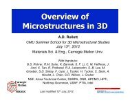
• The objective of this lecture is to introduce 

students to the preferred orientation package 

from Los Alamos (popLA) so that they can 

analyze pole figure data, produce an 

orientation distribution and calculate basic 

properties. 

• Some familiarity with pole figures and 

orientation distributions is assumed.

3 

1. What is a standard sequence of operations to obtain an 

Orientation Distribution (OD) from a set of experimentally 

measured pole figures? 

2. What is the most important check on the quality of the OD 

calculation? 

3. How do you detect problems with defocussing, and what 

practical steps can you take to correct them? 

4. Why is the alignment of the specimen in an x-ray goniometer 

important for subsequent texture analysis? 

5. Why is it helpful to rotate (in-plane) pole figures before 

analysis? 

6. What properties can you calculate with popLA? (This is not 

covered in this lecture – you need to explore the package!).

4 

• popLA, at the moment, is a DOS-based package. 

(Work is in progress to write a new GUI for XP.) The 

basic sequence of steps to use the program for 

analyzing a pole figure data set are as follows. 

– Process the raw PF data (subtract background, apply defocussing 

correction, normalize) 

– Use the series expansion method (fitting of generalized 

spherical harmonics) to preform a preliminary OD analysis of 

the data 

– Use the re-normalized result from above as input to a WIMV 

analysis (calculation of a discrete OD) 

– Plot the results 

– Calculate volume fractions of texture components of interest 

– Calculate inverse pole figures, non-measured pole figures 

– Calculate sets of individual orientations weighted by their fit to 

the OD

POPLA 

Preferred Orientation Package-Los Alamos 

A.D. (Tony) Rollett 

with thanks to Carl Necker, Los Alamos 

National Laboratory, and Raul Bolmaro, 

Rosario Univ., Argentina 

adapted from ICOTOM 15 Workshop, 2008

Preferred Orientation Package Los Alamos

C:/x/popla.bat 

1980s to Present: DOS based coherent set of programs 

works on many PC systems (started on IBM 286 DOS machine) 

Microsoft’s advent of Windows XP and Vista 

finding some issues, particularly with DOS screen capture 

Non-Windows based format not as user friendly to the Windows based world 

LANL contract with University of Rosario, Rosario Argentina 

create a Windows based interface to run popLA 

user friendly interface 

remove programs that were driven by ‘slow’ computer speeds 

improve functionality

Historical information 

Things to keep in mind before using PopLA 

Review classic PopLA with typical data processing scenario 

Introduce the New and Improved PopLA 

A look under the hood – how the critical programs work 

Supplementary tools to be used in concert with PopLA 

What can you do to help improve PopLA?

(IBM 286!) 

Los Alamos thinking…. 

+ 

Automate the process of 

evaluating and presenting 

texture

Fred Kocks John Kallend Tony Rollett 

Gilles Canova 

Rudy Wenk 

Raul Bolmaro 

Carl Necker 

Carlos Tome 

Tayfur Ozturk 

Stuart Wright

Time stamp on many of the critical programs: 1988-1989 

Kocks, Canova, Tome, Rollett, Wright, Computer Code LA- 

CC-88-6 

(Los Alamos, NM: Los Alamos National Laboratory, 1988) 

Kocks, Kallend, Wenk, Rollett, Wright, Computer Code LA- 

CC-89-18 

(Los Alamos, NM: Los Alamos National Laboratory, 1989) 

Minor changes through the early 1990s 

Otherwise: unchanged

typical 5-axis goniometer 

Bragg’s Law 

Proper goniometer alignment required! 

Keep peaks from shifting! 

PopLA is only as good as your measurements! (Garbage in, garbage out)

• Defocusing correction more important with decreasing 2θ and narrower 

receiving slit. 

• Best procedure involves measuring the intensity from a reference 

sample with random texture. 

• If such a reference sample is not available, one may have to correct the 

available defocusing curves in order to optimize the correction. 

• An important point to be aware of is that the exact shape of each 

defocussing curve depends on the material and the machine. The 

material influence is primarily through the diffraction angles (correction 

is more important for small angles). The machine influence is primarily 

through the slit widths (acceptance angle at the detector, e.g.).

1=RD Mark samples with orientations 

Record connection between 

sample nomenclature and 

orientation with goniometer 

reference frame. 

3=ND 2=TD 

popLA assumes a counter-clockwise data 

sequence in files thus UNRAW inverts the 

spin (RAW-EPF) since ‘our’ goniometer 

spins clockwise. Check the sense of rotation 

on your own system! 

Keeping track of these orientations is critical when dealing 

with non-symmetric textures as well as when you write your own 

programs to convert goniometer specific data into popLA format.

16 

How can you tell that the instrument 

and material (sample) axes are not 

aligned? Generally the pole figures 

tell you immediately, especially if any 

plane rolling has occurred during the 

lifetime of the material. 

It can easily happen that the 

sample is mounted in the 

instrument (x-ray 

goniometer, for example) in 

such a way that the natural 

material axes are not aligned 

with the instrument axes.

17 

Caution: if the mis-match between Materials and 

Instrument axes is more complicated than just in the 

X-Y plane, you will have to first compute the OD, then 

re-calculate complete pole figures, then you can use 

the popLA tool that permits out-of-plane rotations 

(page 2, #5). Alternatively, you can generate a 

Weighted List of orientations and rotate all the 

rotations in that list. This tool does not exist in popLA 

at this point so you will have to write your own 

program. 

So, what can you/ should you do 

about this issue? 

Answer: if you expect the texture to 

reveal the inherent material axes 

(that are a consequence of its 

thermomechanical history), then 

make the measurement and perform 

the rotations on the pole figures (in 

the X-Y plane: page 2, #4).

IT MUST BE PERFECT! 

First line is (a26) to include an 8 character name (a limitation) and date? 

Second line: 

Fortran (a5,4f5.1,5i2,2i5,2a5) 

(hkl,DR,RM,DAZ,AZM,IW,JW,IPER,IAVG,IBG,stuff) 

Third line+: 

(1x,18i4) if i>9999 then all data in the pole figure is scaled – IAVG

19 

popLA: preferred orientation package - Los Alamos (Page 1) 

U.F. Kocks, J.S. Kallend, H.R. Wenk, A.D. Rollett, S.I. Wright (April 1995) 

0. QUIT 

1. Get specimen DIRECTORY and VIEW a file 

2. MASSAGE data files: correct,rotate,tilt,symmetrize,smooth,compare 

3. WIMV: make spec.SOD; calculate PFs and inverse PFs; make matrices 

4. HARMONIC analysis: COMPLETE rim (.FUL), get Roe Coeff.file (.HCF) 

5. CONVERSIONS, permutations, transformations, paring 

6. DISPLAYS and plots 

7. Derive PROPERTIES from .SOD or .HCF files, make WEIGHTS file for simul. 

8. DOS (temporary: type EXIT to return)_ 

Please type a number from 0 to 8 -->

20 

DISPLAYS AND PLOTS (popLA page 6) 

0. Quit 

1. Return to Page 1 

------ POLAR REPRESENTATION (Wenk and Kocks) --------- 

DENSITY PLOTS: 

2. POD: colors or gray-shades on VGA 

(with possibility to capture into .PCX file or such) 

or (with less resolution) direct to hp-LASERJET or PS-file 

CONTOUR PLOTS: 

3. OD sections from density files (Wenk program): very slow! 

4. single PF from density file (Wenk program, slow) 

5. single PF from density file (Kallend program, need PP.EXE or hp-plotter) 

DISCRETE ORIENTATION PLOTS: 

6. PFs, points or contours (Tome/Wenk program) 

7. DIORPLOT: all OD sections and projections, compatible with POD 

------ SQUARE SECTIONS (Kallend): cub/hex/tetr.cry.,ort/mono samples 

8. Colors on screen (fast, but limited options). 

9. Contours on hp-Laserjet (needs PP.EXE) or hp-plotter 


21 

POD

22 



0. QUIT 










23 

UNRAW 

MASSAGE DATA FILES (mostly PFs) (popLA page 2) 

0. Quit 


2. Make THEORETICAL defocussing & background file: .DFB (R. Bolmaro) 

3. DIGEST Raw Data (.RAW), with exper.or theor. .DFB: make .EPF 

4. ROTATE PFs or adjust for grid offsets: make .RPF or .JWC 

5. TILT PFs around right axis: make .TPF (T. Ozturk) 

6. SYMMETRIZE PFs: make .QPF or .SPF or .FPF 

7. EXPAND PFs back to full circle (needed for WIMV & harm.): .FPF 

8. SMOOTH PFs or ODs with Gaussian Filter (quad, semi, or full): make .MPF 

9. Take DIFFERENCE between 2 files (PFs or ODs): make .DIF

24 

UNRAW 

DEMO RAW 17,447 10-0-93 8 ¦ Volume in drive C has no label 

olume 

Directory of C:\x\demo16FB ¦ :50a DEMO.RAW 

1 file(s) 17,447 bytes 

0 dir(s) 2,147,155,968 bytes free 

Note: If your data are on a SCINTAG .RR file: use DA5READ to make .RAW 

If they are on a PHILIPS .RAW file, use UNPHIL to make our .RAW 

If they are on an Aachen pole figure file, use AC2LA to make .EPF 

If they are on a RIGAKU .PFG file: use RIG2LA to make our .RAW 

(but you must have a PWD subdirectory into which it puts it: 

compliments of RIGAKU/USA.) 

(BREAK now to do any of the above..., else RETURN) 

Press any key to continue . . . 

Empirical Defocussing Correction 

Note: the sample is assumed to have rotated counter-clockwise 

Data will be sequenced clockwise in .EPF 

Enter name of raw data file (ext .RAW assumed) demo 

Enter name of correction file (ext .DFB assumed)demo

25 

demo Cu rol.90%,pt.reXeX (from Necker' 

(hkl)=(111) Background= 195 Using correction curve 1 

...correcting raw data 

...extrapolating outer ring 

...normalizing. Normalization factor= .088 

...writing corrected data to demo .EPF 





WARNING! Extrapolation gives negative intensities. Values set to 1 









Stop - Program terminated. 

Press any key to continue . . .

26 



0. QUIT 










27 

DISPLAYS AND PLOTS (popLA page 6) 

0. Quit 


------ POLAR REPRESENTATION (Wenk and Kocks) --------- 

DENSITY PLOTS: 

2. POD: colors or gray-shades on VGA 

(with possibility to capture into .PCX file or such) 

or (with less resolution) direct to hp-LASERJET or PS-file 

CONTOUR PLOTS: 

3. OD sections from density files (Wenk program): very slow! 

4. single PF from density file (Wenk program, slow) 

5. single PF from density file (Kallend program, need PP.EXE or hp-plotter) 

DISCRETE ORIENTATION PLOTS: 

6. PFs, points or contours (Tome/Wenk program) 

7. DIORPLOT: all OD sections and projections, compatible with POD 

------ SQUARE SECTIONS (Kallend): cub/hex/tetr.cry.,ort/mono samples 

8. Colors on screen (fast, but limited options). 

9. Contours on hp-Laserjet (needs PP.EXE) or hp-plotter 


28 

quadrants or (circles): 1,2,3-6,7-12 1-2,3-11 (8) 

semi-circles: : 1,2,3-12 1-2,3-11 

Enter the number of plots on page ( 3 

Enter name of data file # 1 --> demo.epf 

Scanning data set identified by: 

demo Cu rol.90%,pt.reX DFB=demo 

(111) 

0 to start with this data set 

n to skip n data sets --> 0 



(200) 



(220) 

Absolute MAXIMUM of all plots in file = 1299. 

Absolute MINIMUM of all plots in file = 0. 

Now you will determine the intensity scale to be used, 

on the basis of 8 major contours. 

(Some choices will later put 2 intervals each.) 

Choose highest contour value 

--> 0

29 


(220) 







--> 800 

-- How many major contours below intensity 1.0 ? 

 

--> 1 

MAJOR CONTOURS will be at (times random): 

8.00 

5.66 

4.00 

2.83 

2.00 

1.41 

1.00 

.71 

HIGH resolution. Contours: Y 

0: OK; 1: try again --> 0

30 

Plot with GMT: 

Plot with popLA:

31 



0. QUIT 










32 

ROTATE 


0. Quit 










33 

Directory of C:\x\demo16FB ¦ :59a DEMO.EPF 



ROTATE POLE FIGURES AND/OR CHANGE GRID 

Program by John Kallend 

1. Symmetry analysis and rotation about center 

2. Change grid azimuth offset (JW) 

3. Change grid polar and azimuth offset (IW,JW) 

4. Invert spin 

Enter 1, 2, 3, or 4 --> 1 

Input file (with .ext, default .EPF): demo 

111 demo Cu rol.90%,pt.reX DFB=demo 



SUGGESTED ROTATION 1.8 DEGREES 

Is this ok? Y 

ROTATE

34 

This step required to bring material axes in line with 

Instrument axes, as discussed previously. 

1.8 degrees

35 

HARMONIC ANALYSIS (popLA page 4) 

0. Quit 


Find harmonic coefficients .HCF, completed PFs (.FUL) for: 

2. Cubic crystal system 

3. Hexagonal, tetragonal or orthorhombic crystal system 

4. Compute SOD or COD from harmonic coefficients (slow!) 

5. Recalculate pole figures .HPF 

6. Inverse pole figures .HIP 

7. List harmonic coefficients to screen or printer 

Note: To convert Aachen-format Bunge coeffs. to Kallend's binary 

Roe coeff.file .HCF: use AC2Wlmn (outside this menu) - 

Also need FAKTOR.CtW (J. Hirsch) 

8. Establish coefficients for a given TRANSFORMATION 

9. Apply TRANSFORMATION to given coefficients 


36 

Harmonic Pole Figure Analysis (Cubic) 

Enter name of data file (default .epf): demo 

1demo Cu rol.90%,pt.reX 

3 Pole figures read in. 

How many iterations on missing parts? 9 

CUBIC ODF ANALYSIS FOR demo 

Sample symmetry: 

0. Orthorhombic 

1. Mirror perpendicular to Z 

Enter 0 or 1==> 0 

Error output to: 

1. printer 

2. screen 

Enter 1 or 2 ==> 2 

CUBAN2

37 

200 Reflection. Trunc. error = .36 Normalization = .10E+01 

220 Reflection. Trunc. error = .39 Normalization = .10E+01 

Severity = 1.712. Generated to l = 22 

ERROR ESTIMATES: 1. Polefigures 

L MEAN 111 200 220 

0 .228E-06 .225E-06 .233E-06 .225E-06 

2 .204E-02 .155E-02 .247E-02 .198E-02 

4 .245E-02 .255E-02 .301E-02 .155E-02 

6 .146E-02 .201E-02 .114E-02 .101E-02 

8 .162E-02 .111E-02 .149E-02 .210E-02 

10 .127E-02 .113E-02 .716E-03 .174E-02 

12 .622E-03 .869E-03 .181E-03 .610E-03 

14 .124E-02 .120E-02 .111E-02 .139E-02 

16 .706E-03 .145E-03 .539E-03 .109E-02 

18 .545E-03 .786E-03 .306E-03 .424E-03 

20 .572E-03 .556E-03 .355E-03 .740E-03 

22 .764E-03 .665E-04 .591E-03 .118E-02 

ALL .113E+00 .106E+00 .103E+00 .127E+00 

2. Estimated avg. error in ODF .38 

RE-ESTIMATING MISSING PARTS OF POLEFIGURES 

Writing harmonic coefficients to demo .HCF 

Print out Wlmn coefficients ? Y

38 


Plot with popLA:

39 



0. QUIT 










40 

The 3 

WIMV 

options 

WIMV Analysis (popLA page 3) 

0. Quit 


WIMV: make .SOD and recalc. pole figures .WPF -- for: 

2. cubic, tetra-,hexagonal crystals; sample diad: up to 3 PFs, 13 poles WIMV 

3. trigonal cry.,gen'l.sample sym.,or higher: up to 7 PFs, 25 poles BWIMV 

4. orthorhombic crystals; sample Z-diad: up to 7 PFs, 25 poles OWIMV or WIMV386 

**or: orthorh./gen'l./7/25 **requires 386, DOS 5, and 4MB memory** 

Recalculate POLE FIGURES (even non-measured ones): make .APF - 

5. using .WIM matrix for the desired PFs (up to 3, 13 poles) SOD2PF 

6. using .BWM or .WM3 matrix for the desired PFs (up to 7, 25 poles) 

7. Calculate INVERSE pole figures from .SOD: .WIP 

OSOD2PF 

(So far assumes tetragonal crystal symmetry) 

SOD2INV 

8. Make WIMV pointer matrix for new crystal structure and set of PFs ** 

9. Make WIMV pointer matrix for any INVERSE pole figures: make .WMI 

Please type a number from 0 to 9 --> INVGEN 

**WIMVGEN/BWIMVGEN/WGEN386; see later slides for notes on pointer matrices

42 

Note: the “FON” is 

the name for the 

uniform (“random”) 

background level; 

“raising the FON” 

means that the 

program will try to 

maximize this 

level. In practice, 

this makes little 

difference to the 

outcome. 

ODF ANALYSIS - WIMV ALGORITHM 

COPYRIGHT (C) 1987,1988 JOHN S. KALLEND 

*** Version September 1993 *** 

Enter the name of the wimv matrix (?.WIM) 

[Default is CUBIC] ==>CUBIC 

Name of data file (default extension .epf): demo.ful 

Sample Symmetry is: 

0. Orthorhombic 

1. Diad on Z 

Enter 0 or 1 ==> 0 

demo Cu rol.90%,pt.reX 

111 5.0 90.0 5.0360.0 1 1 2-1 3 100 72 

200 5.0 90.0 5.0360.0 1 1 2-1 3 100 72 

220 5.0 90.0 5.0360.0 1 1 2-1 3 100 72 

The minimum pole figure intensity is .01 

Do you wish to raise the Fon? N

43 

Iteration 2 in progress 

Sharpening may cause larger error in iteration 3 

Texture Strength (m.r.d.): 2.0 

(= square-root of "Texture Index") 

Iteration 2 estimated OD error (%) = 36.1 













Continue? Y

44 

Continue? Y 




Continue? Y 




Continue? Y 




Continue? n 

Normalization factor: .99 

In output file, angles increase from 0 in nomenclature of 

1. Kocks (need this one for WEIGHTS) 

2. Roe/Matthies 

3. Bunge (rotates plot +90 deg.) 

Enter 1,2, or 3 ==> 1

45 

There are 3 “flavors” of the WIMV algorithm. Each successive 

version was developed to have more capability but the older 

versions were kept because they required less memory and ran 

faster (no longer an issue). We recommend that you always use 

the 3 rd option (menu item 4) which is the most capable. The 

executable is called OWIMV.EXE or, possibly, 

WIMV386.EXE, depending on your system. 

In order to use WIMV, one must have a “pointer matrix” which 

is just a list of which cells in pole figure space are connected to 

which cells in orientation space. Just as there are 3 versions of 

WIMV itself, so too there are 3 versions of the pointer 

generation program. WIMVGEN goes with WIMV.EXE; 

BWIMVGEN goes with BWIMV.EXE; WGEN386 goes with 

OWIMV (or WIMV386).

46 

To run the pointer matrix generation programs, you need to 

know the crystal symmetry (cubic, hexagonal, trigonal …), and 

any relevant ratios of lattice parameters (e.g. c/a for hcp), and 

which pole figures you want to be able to analyze. The 

program will guide you through how to enter the Miller indices 

for each pole figure (and it has certain preferences as to how to 

enter those values, e.g. 1 1 0, not 2 2 0).

48 

QUAD4 


0. Quit 










49 

DEMO QPF 4,890 10-0-93 11 ¦ Volume in drive C has no label 

olume 

Directory of C:\x\demo16FB ¦ :32a DEMO.QPF 



File not found 

Directory of C:\x\demo16FB ¦ Volume in drive C has no label 

olume 

2,147,155,968 bytes free 

Make full pole figure from quadrant or semi 

Program by John Kallend 

Enter name of data file (with extension) : demo.wpf

50 


Plot with popLA:

51 

******************************************************** 

To return to program, type EXIT (from SAME subdirectory) 

******************************************************** 

Microsoft(R) Windows 98 

(C)Copyright Microsoft Corp 1981-1999. 

C:\x\demo>copy demo.ful+demo.fpf demo.cmb

54 

quadrants or (circles): 1,2,3-6,7-12 1-2,3-11 (8) 

semi-circles: : 1,2,3-12 1-2,3-11 

SOD2INV 

Enter the number of plots on page ( 3 

Enter name of data file # 1 --> demo.wip 


demo Cu rol.90%,pt.reXcalculated from SOD 8-OCT-93 strength= .00 

SOP3 PROJ 

0 to start with this data set 

n to skip n data sets --> 0 



SOP2 PROJ 



SOP1 PROJ 

THE FILE CONSISTS OF SOD SECTIONS: 

0 Plot default (full or quarter circles) 

1 Plot cubic inverse pole figures 

2 Plot tetragonal inverse pole figures 

3 Plot hexagonal inverse pole figures 

4 Plot trigonal inverse pole figures 

1

55 


Plot with popLA:

56 



0. QUIT 










57 

CONVERSIONS of SODs, HCFs, and discrete angles files (popLA page 5) 

0. QUIT 

1. RETURN to Page 1 

--- ORIENTATION DENSITY FILES --- 

2. Permute axes in .SOD 

3. Make .COD from .SOD file (or .CHD from .SHD) 

4. Make OBLIQUE sections from .SOD file: .SON,.CON, or .SHN,.CHN from .SHD 

(Note: no projections; use the one from end of .COD or .SOD) 

5. Pare to SUBSET for display: make .SOS or .COS (or .SHS,.CHS) 

--- DISCRETE ORIENTATION FILES --- 

6. Convert generic MILLER INDICES to any Euler angles 

7. DIOR: Add crystal and sample symmetries, permute axes, change 

angle convention, or make DENSITY file from DISCRETE grain file 

SOD2COD 

PARE

58 demo Cu rol.90%,pt.reX 37 WIMV iter: 1.7%,Fon= 0 2 

SODK Psi= 90.0 


demo Cu rol.90%,pt.reX 37 WIMV iter: 1.7%,Fon= 0 2 

SOP3 Psi=PROJ 

THE FILE CONSISTS OF SOD SECTIONS: 

0 Plot default (full or quarter circles) 

1 Plot cubic inverse pole figures 

2 Plot tetragonal inverse pole figures 

3 Plot hexagonal inverse pole figures 

4 Plot trigonal inverse pole figures 

0 







--> 1600 

-- How many major contours below intensity 1.0 ? 

 

--> 2

61 

The conventional plotting approach is to use Cartesian (square) plots, 

as you find in most papers and books. 

We illustrate plotting using the programs smoothsod[.f90] (for 

smoothing orientation distributions with a Gaussian filter, and 

sodcon[.f] for contour plotting. The latter has options to plot with 

line contours, or solid colour. It can also plot ODs for hexagonal 

materials where one generally wants to limit the third angle to the 

range 0-60° because of crystal symmetry. These are available in 

texture_subroutines on my website. The latter program must be 

compiled with the package of routines called psplot.txt, which you 

can find at www.nova.edu/ocean/psplot.html . 

To compile fortran programs, try using gfortran on Macs 

(hpc.sourceforge.net) or g95 on PCs (www.g95.org).

62 

unsmoothed Smoothed (5°)

63 


64 

See neon.materials.cmu.edu/texture_subroutines for programs 

x = φ 1 , y = Φ , z = φ 2 

Use SOD2vtk.f to get a VTK file 

for 3D viewing

65 

PROPERTIES (popLA page 7) 

0. Quit 


2. Assign WEIGHTS to discrete grains file from .SOD 

_ (Need Kocks style Euler angles in both .SOD and TEXfile - 

_ can convert the latter in DIOR, p.5,#7) 

3. Average ELASTIC properties (Reuss, Voigt, Hill, self-consistent) 

(Program by C. Tome) Input ELTEX.DAT, ELMOD.DAT; out ELOUT?.DAT 

4. SIMULATION of polycrystal PLASTICITY from weighted grains file - 

LApp code: with rate sensitivity and grain shape effects, 

for all crystal and sample symmetries (not much twinning): 

calculate current yield surface, Lankford coefficients; 

predict texture development, Taylor factors, 

stress/strain curves for all straining paths. Up to 1152 grains. 

SHEET properties directly from harmonic coefficients (Kallend) 

(only for orthotropic plane strain, cubic metals): 

LANK 

5. Yield locus section (11,22) for any angle in plane (Bishop-Hill) 

6. Lankford coefficients (Hosford-Backofen model) 


66 

Plastic anisotropy calculations for FCC, BCC metals 

from harmonic coefficients. 

Program by John Kallend (C)1969 

What is the specimen name (.HCF Assumed)? demo 

Plasticity data for demo Cu rol.90%,pt.reX 

RESTRICTED (R) or PENCIL (P) glide ? 

Enter P or R: ==> r 

Parameters calculated: 

M = Taylor Factor 

R = Lankford parameter 

qmin = width/length strain 

beta = ratio of plane strain strengths Mez=o/Mey=o 

Restricted glide 

Angle M R qmin Beta 

0 3.16 .87 .46 1.00 

15 3.13 .82 .45 .99 

30 3.10 1.19 .54 1.02 

45 3.04 1.62 .62 1.03 

60 2.99 1.31 .57 1.03 

75 3.01 .89 .47 .99 

90 3.05 .82 .45 .96 

Press any key to continue . . .

67 

PROPERTIES (popLA page 7) 

0. Quit 


WEIGHTS 

2. Assign WEIGHTS to discrete grains file from .SOD 

_ (Need Kocks style Euler angles in both .SOD and TEXfile - 

_ can convert the latter in DIOR, p.5,#7) 

3. Average ELASTIC properties (Reuss, Voigt, Hill, self-consistent) 

(Program by C. Tome) Input ELTEX.DAT, ELMOD.DAT; out ELOUT?.DAT 

4. SIMULATION of polycrystal PLASTICITY from weighted grains file - 

LApp code: with rate sensitivity and grain shape effects, 

for all crystal and sample symmetries (not much twinning): 

calculate current yield surface, Lankford coefficients; 

predict texture development, Taylor factors, 

stress/strain curves for all straining paths. Up to 1152 grains. 

SHEET properties directly from harmonic coefficients (Kallend) 

(only for orthotropic plane strain, cubic metals): 

5. Yield locus section (11,22) for any angle in plane (Bishop-Hill) 

6. Lankford coefficients (Hosford-Backofen model) 


68 

Directory of C:\x\demo16FB ¦ Volume in drive C has no label 

olume 

2,147,155,968 bytes free 

******************************************************************* 

For discrete grains files, use the following (in c:\x): 

filename min.cry.sym min.sam.sym use #grains: 

-------- ----------- ----------- ----------- 

texRAN any any any(1000) 

texRAN.WTS tetragonal Z-diad all(1000) 

texISO.wts tetragonal any/Z-diad/ortho. 1024/512/256 

texCUB.wts cubic any/Z-diad/ortho. 3072/1536/768 

...here, average triplets, so final # is 1024/512/256 

texREG.wts tetragonal diad on Z or Y 3456 (/3=1152 for cubic) 

orthotropic 1728 (/3=576 for cubic) 

fiber which stays 192 (/3=64 for cubic) 

******************************************************************* 

Intensity file (w/ext:.SOP or .S?D, default=.SOD): demo.sod

69 

Discard grains below a certain weight? Which? 0. 

.1 

texran :use any portion (only file when less than tetr.cry.sym.) 

Evm F11 F12 F13 F21 F22 F23 F31 F32 F33 

0.000 1.000 0.000 0.000 0.000 1.000 0.000 0.000 0.000 1.000 

Kocks:Psi Theta phi weight (up to 6 state parameters, f8.2) XYZ= 1 2 

Is this a file of triplets to be averaged? 0 

How many orientations total? 1500 

Do you wish to bring grains from outside the irreducible area 

into it, by applying 360/PHImax-fold crystal Z-axis? 

(Use 0 with TEXLAT.WTS, TEXISO.WTS, TEXCUB.WTS)-> 1 

Writing file 

demo .wts 

681 grains written 

Volume fraction .01 discarded 

You may wish to rerun with different limit on weights... 

For grain-shape effect, you must manually adjust F in .WTS file! 

(Also, you may wish to record vol.fraction discarded in 1st line.)

70 

• A frequent problem with using popLA for the first time concerns the main 

graphics program, POD. This program expects to see a file called 

PODIN. This file merely serves to record what parameters were used 

the last time that POD was run. 

• The file is available from Rollett’s popLA page: 

neon.materials.cmu.edu/rollett/popLA 

• Even if you have the file present in your \X directory, you will still need to 

copy it into whatever directory you are working in 

(copy C:\X\PODIN .). 

• Note that the main issue with POD under XP is that “PrintScreen” no 

longer works. An alternative approach to graphics is to use postscriptbased 

graphics. Programs (scripts) exist to plot pole figure information 

with GMT [Generic Mapping Tools, http://gmt.soest.hawaii.edu/ ]. The 

script is called “Draw_Stereograms” and can be found in 

texture_subroutines in a folder called “plotting with GMT” on my website. 

There is also a small conversion program called “pf2GMT.f” that converts 

data files to GMT format, for Draw_stereograms to use as input. 

• Another alternative is to use DOSBox, which is a DOS emulator freely 

available just type “DOSBox” into Google and follow the link(s).

71 

• DFB files contain data on defocussing (and 

background) corrections. An example of 

how the values vary with angle is shown on 

the right of the slide. 

• An important point to be aware of is that the 

exact shape of each defocussing curve 

depends on the material and the machine. 

The material influence is primarily through 

the diffraction angles (correction is more 

important for small angles). The machine 

influence is primarily through the slit widths 

(acceptance angle at the detector, e.g.). 

• The best way to obtain a defocussing curve 

for your particular material is to measure 

pole figures on a randomly oriented sample 

of that same material. 

• Whenever you change material, or 

diffractometer, you can expect your 

defocussing corrections (and therefore DFB 

file) to change.

72 

• To illustrate the effect of varying the defocussing, we analyze a data set 

for a steel sample with two different defocussing corrections and 

examine the impact on the quality of the OD calculation. The source of 

the 1st DFB is unknown and the curves cross in a rather unlikely 

fashion; the 2nd was generated with MAKEDFB (option #2 on page 2) 

using the theta values appropriate to Fe, Cu-Ka radiation, a slit width of 

0.1° and a peak width of 1°.

73 

• Now we show the corrected . EPF files. 

Note the more uniform intensity going out to the edges 

of the PFs in the second set.

74 

Note that the harmonic 

analysis produces rather 

similar results because of 

the renormalization of the 

PFs. 

• And the .FUL 

files from 

performing a 

harmonic 

analysis:

75 

Note that using an incorrect 

defocussing correction will be 

most likely to give problems if 

you use the WIMV analysis 

directly on .EPF files. First 

applying the harmonic analysis 

and then using the .FUL dataset 

as input to WIMV is much more 

likely to be correctly normalized. 

• And, finally, 

the .WPF files (from 

applying the WIMV 

analysis, no sample 

symmetry):

76 

• Please find the description in 

Converting_XPert_to_POPLA_format_KB.doc 

that is posted on the course website 

• Note that the program provided by Phillips (now 

PanAlytical) produces a popLA *.raw file that has 

minor but significant errors on the second line of 

each file. These must be corrected before 

processing the data with popLA.

78 


80 


./pf2GMT demo.wip 

[ program digests the inverse PF data, converts to GMT format with 

{longitude,latitude,intensity}, giving 3 (typically) files with names 

demo_wip1.gpf, demo_wip2.gpf, demo_wip3.gpf ] 

./Draw_Stereograms 3 demo_wip IP \ 

( wysiwyg/gray/polar/rainbow low-contour high-contour step stereo/ 

equal/ortho CUBIC/HEX/ORT ) 

Note that the script uses clipping to obtain only the SST (standard 

stereographic triangle).

82 

• There are various issues connected with open source graphics. 

• GMT is best suited to Unix systems; on Windows the advice is to run it 

in a Unix window (Cygwin). Installation of GMT on a Mac requires prior 

installation of Develop Tools (including X11) - this is easy; then you 

must generate a script and run it - mildly scary when doing it for the first 

time. Also available from port (http://www.macports.org/); once “port” is 

installed, you can get GMT via “sudo port install gmt”. Once you have it 

installed, a long list of programs become available for the various 

processing steps - Draw_stereograms automates this for you. 

• The main reason to use GMT is that it handles spherical data very 

gracefully; does not require a regular grid, knows every standard 

projection, can smooth data, and allows annotation. 

• PSPLOT is a simpler package because it is only a set of subroutines. 

As with most such packages, the authors like you to register as a user 

so that they that you are using it, and so that they can get the credit for 

the use. Significantly more effort is required, however, to write the 

Fortran code to make use of the capability and generate plots. Paul 

Lee (Ph.D., CMU/MSE, 1999) is credited with writing the original 

version of SODCON.

83 

• A team in Argentina, headed up by Raúl Bolmaro, took popLA 

and embedded it in a GUI using wxpython. The name of the 

package is wxpopla. Various notes about how to use it are as 

follows. The key point is that it only runs under Windows XP, 

not, for example, under Windows 7. 

• A useful approach is to use DOSBOX as a container/wrapper for 

either the DOS version of popLA, or wxpopla. Since wxpopla 

requires wxpython as its environment, it is essential to follow the 

instructions in the installation manual (posted on my website 

separately from the .rar archive of wxpopla). 

• One person (2011) was able to run wxpopla with the following 

configuration: 

Windows XP mode on a Windows 7 64-bit laptop (Integration 

Features Disabled, essential to run 32-bit color for wxPopla to 

function).

84 

• Any Windows installation, preferably XP (needs more testing in older builds) Python 2.5 or better (not 3.0 

until more tests are made) wxPython 2.8 Unicode or better 800x600 resolution at 32 bits (True colors 

display) Roughly 25mb of RAM and a few Mb of free disk space in C: for temporary files. 

• Notes: 

============== 

• The Viewer, Project and Help panels are non-functional. 

• The "open in external editor" function works as long as Windows is installed in "C:\Windows". The program 

is not dependant of this, but currently there is no user-friendly way to modify the program to execute's path. 

• In very low resolutions or window sizes a yet-to-be-fixed bug can sometimes stop the program from 

displaying its panels correctly. 

• Maximizing or resizing the window to sensible dimensions solves the problem. 

• The GUI's colors are user-modifiable, although no facility to change them exists as of yet. 

• Some tools might not have all supported input formats available in the Open dialog. Temporarily, selecting 

"All files (*.*)" will allow you to select previously inaccessible files. 

• The console still needs a lot of refinement. 

================= 

• Because of fixed, absolute path names in the programs, the following files must be downloaded separately 

into the C:\X\ directory: 

PNORM.CFS 

SINCOS.CFS 

PCOEFS.V33. 

• In the OWIMV wizard, symmetry is spelled "simmetry”. 

• wxpopLA occasionally crashes when changing packages.

85 

• Basic sequence demonstrated that 

takes you from RAW pole figures, as 

measured on an x-ray goniometer to an 

Orientation Distribution. 

• Many more functions available.

A.D. Rollett, Carnegie Mellon Univ.

You also want an ePaper? Increase the reach of your titles

Delete template?

Save as template?