Polycrystal Plasticity - Multiple Slip

Carnegie
Mellon
MRSEC
1
Polycrystal Plasticity -
Multiple Slip"
27-750
Texture, Microstructure &
Anisotropy
A.D. Rollett,
H. Garmestani (GaTech),
G. Branco (FAMU/FSU)
Last revised: 21 st Oct. ‘11
Jump to first page

2
Objective"
The objective of this lecture is to show how
plastic deformation in polycrystals requires
multiple slip in each grain.
Further, to show how to calculate the
distribution of slips in each grain of a
polycrystal (principles of operation of Los
Alamos polycrystal plasticity, LApp).
Requirements:
Dislocation controlled plastic strain
Mechanics of Materials
Continuum Mechanics

3
Questions"
What is the difference between single slip and multiple slip in terms of
boundary conditions?
What is “deviatoric stress” and why does it have 5 components?
How does the von Mises criterion for ductility relate to the 5 components of
deviatoric stress and strain?
How does the Bishop-Hill theory work? What is the input and output to the
algorithm? What is meant by the “maximum work” principle?
What is the Taylor factor (both definition and physical meaning)?
Why is the rate-sensitive formulation for multiple slip useful above and
beyond what the Bishop-Hill approach gives?
What is it that causes/controls texture development?
On what quantities is lattice reorientation based (during multiple slip)?
How can we compute the macroscopic strain due to any given slip system?
How can we compute the resolved shear stress on a given slip system,
starting with the macroscopic stress (tensor)?
What does Bishop & Hill state of stress mean (what is the physical
meaning)? [Each B&H stress state (one of the 28) corresponds to a corner
of the single xtal yield surface that activates either 6 or 8 slip systems
simultaeneously]

4
References"
Kocks, Tomé & Wenk: Texture & Anisotropy (Cambridge); chapter
8, 1996. Detailed analysis of plastic deformation and texture
development.
Reid: Deformation Geometry for Materials Scientists, 1973. Older
text with many nice worked examples. Be careful of his examples
of calculation of Taylor factor because, like Bunge & others, he
does not use von Mises equivalent stress/strain to obtain a scalar
value from a multiaxial stress/strain state.
Hosford: The Mechanics of Crystals and Textured Polycrystals,
1993 (Oxford). Written from the perspective of a mechanical
metallurgist with decades of experimental and analytical experience
in the area.
Khan & Huang: Continuum Theory of Plasticity. Written from the
perspective of continuum mechanics.
De Souza Neto, Peric & Owen: Computational Methods for
Plasticity, 2008 (Wiley). Written from the perspective of continuum
mechanics.
Key Papers: Taylor G., (1938) Plastic strain in metals, J. Inst.
Metals (U.K.) 62 307 ; Bishop J and Hill R (1951) Phil. Mag. 42
1298.

5
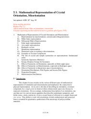
Output of LApp"
Figure shows pole
figures for a simulation
of the development of
rolling texture in an fcc
metal.
Top = 0.25 von Mises
equivalent strain; 0.50,
0.75, 1.50 (bottom).
Note the increasing
texture strength as the
strain level increases.
Increasing strain

6
The Theory depends upon:
Basic Considerations"
The physics of single crystal plastic deformation;
relations between macroscopic and microscopic quantities
( strain, stress ...);
The mathematical representation and models
Initially proposed by Sachs (1928), Cox and Sopwith (1937),
and Taylor in 1938. Elaborated by Bishop and Hill (1951).
Self-Consistent model by Kröner (1958, 1961), extended by
Budiansky and Wu (1962).
Further developments by Hill (1965a,b) and Lin (1966, 1974,
1984) and others.
• Read Taylor (1938) “Plastic strain in metals.” J. Inst. Metals (U.K.) 62, 307. - available
as: Taylor.1938.pdf

7
Basic Considerations"
Sachs Model (previous lecture on single crystal):
- All single-crystal grains with aggregate or polycrystal
experience the same state of stress;
- Equilibrium condition across the grain boundaries satisfied;
- Compatibility conditions between the grains violated, thus,
finite strains will lead to gaps and overlaps between grains;
- Generally most successful for single crystal deformation with
stress boundary conditions on each grain.
Taylor Model (this lecture):
- All single-crystal grains within the aggregate experience the
same state of deformation (strain);
- Equilibrium condition across the grain boundaries violated,
because the vertex stress states required to activate multiple slip
in each grain vary from grain to grain;
- Compatibility conditions between the grains satisfied;
- Generally most successful for polycrystals with strain
boundary conditions on each grain.

8
Sachs versus Taylor"
Diagrams illustrate
the difference
between the Sachs
iso-stress
assumption of
single slip in each
grain (a, c and e)
versus the Taylor
assumption of isostrain
with multiple
slip in each grain (b,
d).
iso-stress iso-strain

9
Sachs versus Taylor:
Single versus Multiple Slip"
External Stress or External Strain
Increasing strain
σ ˙
=
τ γ
˙ ε =
1
cosλcosφ
Small arrows
indicate identical
stress state in
each grain
Each grain
deforms according
to which single
slip system is
active
D = E T dγ
Small arrows
indicate variable
stress state in
each grain
Multiple slip (with 5
or more systems) in
each grain satisfies
the externally
imposed strain, D

10
Taylorʼs Multiple Slip"
Shows how each grain must conform to the macroscopic
strain imposed on the polycrystal

11
Example of Slip Lines at Surface
(plane strain stretched Al 6022)"
T-Sample at 15% strain
PD // TD
PSD // RD
Note how each grain
exhibits varying degrees
of slip line markings.
Although any given
grain has one dominant
slip line (trace of a slip
plane), more than one is
generally present.
Taken from PhD
research of Yoon-Suk
Choi on surface
roughness development
in Al 6022

12
Notation: 1"
Strain, local: E local ; global: E global
Slip direction (unit vector): b or s
Slip plane (unit) normal: n
Slip tensor, m ij = b i n j
Stress (tensor or vector): σ
Shear stress (usually on a slip system): τ
Shear strain (usually on a slip system): γ
Stress deviator (tensor): S
Rate sensitivity exponent: n
Slip system index: s or α
Note that when an index (e.g. of a Slip system, b (s) n (s) ) is
enclosed in parentheses, it means that the summation
convention does not apply even if the index is repeated in the
equation.

13
Notation: 2"
Coordinates: current: x; reference X
Velocity of a point: v.
Displacement: u
Hardening coefficient: h (dσ = h dγ )
Strain, ε
measures the change in shape
Work increment: dW
do not confuse with spin!
Infinitesimal rotation tensor: Ω
Elastic Stiffness Tensor (4th rank): C

14
Plastic spin: W
Notation: 3"
measures the rotation rate; more than one
kind of spin is used:
“Rigid body” spin of the whole polycrystal: W
“grain spin” of the grain axes (e.g. in
torsion): W g
“lattice spin” from slip/twinning (skew
symmetric part of the strain): W c .
Rotation (small): ω

15
Notation: 4"
Deformation gradient: F
Measures the total change in shape
(rotations included).
Velocity gradient: L
Tensor, measures the rate of change of the
deformation gradient
Time: t
Strain rate: D
symmetric tensor; D = symm(L)
€
≡ ˙ ε ≡ dε
dt
€
F ij = ∂x i
∂X j

16
Dislocations and Plastic Flow"
At room temperature the dominant mechanism of plastic deformation
is dislocation motion through the crystal lattice.
Dislocation glide occurs on certain crystal planes (slip planes) in
certain crystallographic directions (// Burgers vector).
A slip system is a combination of a slip direction and slip plane
normal.
A second-rank tensor (m ij = b i n j ) can associated with each slip
system, formed from the outer product of slip direction and normal.
The resolved shear stress on a slip system is then given by τ = m ij σ ij .
The crystal structure of metals is not altered by the plastic flow.

17
Schmidʼs Law"
Initial yield stress varies from sample to sample depending on, among
several factors, the relation between the crystal lattice to the loading axis
(i.e. orientation, written as g).
The applied stress resolved along the slip direction on the slip plane (to
give a shear stress) initiates and controls the extent of plastic deformation.
Yield begins on a given slip system when the shear stress on this system
reaches a critical value, called the critical resolved shear stress (crss),
independent of the tensile stress or any other normal stress on the lattice
plane (in less symmetric lattices, however, there may be some dependence
on the hydrostatic stress).
The magnitude of the yield stress depends on the density and arrangement
of obstacles to dislocation flow, such as precipitates (not discussed here).
Definition of slip plane, direction and systems
continued

18
Crystallography of Slip"
Slip occurs most readily in specific directions on certain
crystallographic planes.
Slip plane – is the plane of greatest atomic density.
Slip direction – is the close-packed direction within the slip plane.
Slip system – is the combination of preferred slip planes and slip
directions (on those specific planes) along which dislocation motion
occurs. Slip systems are dependent on the crystal structure.

19
Crystallography of Slip in fcc"
Example: Determine the slip system for the (111) plane in a fcc
crystal and sketch the result.
The slip direction in fcc is
The proof that a slip direction [uvw]
lies in the slip plane (hkl) is given by
calculating the scalar product:
hu + kv + lw =0

20
Slip Systems in fcc, bcc, hcp"
The slip systems for FCC, BCC and HCP crystals are
For this lecture we will focus on FCC crystals only
Note:
In the case of FCC crystals we can see in the table that there are 12 slip
systems. However if forward and reverse systems are treated as
independent, there are then 24 slip systems.

21
Elastic vs. Plastic Deformation"
Selection of Slip Systems for Rigid-Plastic Models
Assumption – For FPD, the elastic deformation rate is
usually small when compared to the plastic deformation
rate and thus it can be neglected.
Reasons:
The elastic
deformation is
confined to the
ratio of stress to
elastic modulus
Perfect plastic materials -
equivalent stress = initial
yield stress
For most metals – initial
yield stress is 2 or 3 orders
of magnitude less than the
elastic modulus –
ratio is

22
Determination of Slip Systems"
Selection of Slip Systems for Rigid-Plastic Models
Once the elastic deformation rate is considered, it is
reasonable to model the material behavior using the
rigid-plastic model given by:
D = D p = m α
n
∑ ˙
α=1
where
n is ≤ to 12 systems (or 24 systems – forward and reverse )
considered independent
Note: D can expressed by six components ( Symmetric Tensor)
Because of the condition - tr(D) = Dii = 0
, only five out of
€ the six components are independent.
€
γ α

23
Von Mises criterion"
Selection of Slip Systems for Rigid Plasticity Models
As a consequence of the condition
tr(D) = Dii
=
the number of possible active slip systems (in cubic metals) is greater
than the number of independent components of the tensor strain rate
D p , from the mathematical point of view (under-determined system), so
any combination of five slip systems that satisfy the incompressibility
condition can allow the prescribed deformation to take place. The
requirement that at least five independent systems are required for
plastic deformation is known as the von Mises Criterion. If less than 5
independent slip systems are available, the ductility is predicted to be
low in the material. The reason is that each grain will not be able to
deform with the body and gaps will open up, i.e. it will crack. Caution:
even if a material has 5 or more independent systems, it may still be
brittle (e.g. Iridium).
0

24
Minimum Work Principle"
Proposed by Taylor in (1938).
The objective is to determine the combination of shears or slips that
will occur when a prescribed strain is produced.
States that, of all possible combinations of the 12 shears that can
produce the assigned strain, only that combination for which the
energy dissipation is the least is operative.
The defect in the approach is that it says nothing about the activity or
resolved stress on other, non-active systems (This last point was
addressed by Bishop and Hill in 1951).
Mathematical n
statement: τ c
∑ ˙
α=1
Bishop J and Hill R (1951) Phil. Mag. 42 1298
n
∑ *
˙ γ
*
α
α=1
γ α ≤ τ α
To be continued

25
Minimum Work Principle
Here,
˙
γ - are the actually activated slips that produce D.
α
*
˙ γ α - is any set of slips that satisfy tr(D)=Dii = 0, but are operated by the
corresponding stress satisfying the loading/unloading criteria.
τ c
€
Minimum Work Principle"
n
∑τ ˙ γ ≤ τ
*
c α α
α=1
α=1
- is the (current) critical resolved shear stress (crss) for the material
(applies on any of the αth activated slip systems).
- is the current shear strength of (= resolved shear stress on) the αth τ
*
α
geometrically possible slip system that may not be compatible with the
externally applied stress.
n
∑ ˙
γ
*
α

26
€
Recall that in the Taylor model all the slip systems are
assumed to harden at the same rate, which means that
and then,
€
Minimum Work Principle"
n
τ = τ
*
c α
˙ γ α ∑ ≤ ˙
α=1
n
∑
α=1
γ
*
α
Note that, now, we have only 12 operative slip systems once
the forward and reverse shear strengths (crss) are
considered to be the same in absolute value.

27
Minimum Work Principle"
n
˙ γ α ∑ ≤ ˙
α=1
n
∑
α=1
γ
*
α
Thus Taylor’s minimum work criterion can be summarized
as in the following: Of the possible 12 slip systems,
only that combination for which the sum of the
€ absolute values of shears is the least is the
combination that is actually operative!
The uniformity of the crss means that the minimum work
principle is equivalent to a minimum microscopic shear
principle.

28
Stress > CRSS?"
The obvious question is, if we can find a
set of microscopic shear rates that satisfy
the imposed strain, how can we be sure
that the shear stress on the other, inactive
systems is not greater than the critical
resolved shear stress?
This is not the same question as that of
equivalence between the minimum work
principle and the maximum work approach
described later in this lecture.

29
Stress > CRSS?"
The work increment is the (inner) product of the
stress and strain tensors, and must be the same,
regardless of whether it is calculated from the
macroscopic quantities or the microscopic quantities:
For the actual set of shears in the material, we can
write (omitting the “*”),
where the crss is outside the sum because it is
constant.
[Reid: pp 154-156]

30
Stress > CRSS?"
Now we know that the shear stresses on
the hypothetical (denoted by “*”) set of
systems must be less than or equal to the
crss, τ c , for all systems, so:
This means that we can write:

31
Stress > CRSS?"
However the LHS of this equation is equal
to the work increment for any possible
combination of slips, δw=σ ijδε ij which is
equal to τ c Σ αδγ α , leaving us with:
So dividing both sides by τc allows us to
write:
∑δγ ≤ δγ *
α
∑ Q.E.D.
α

€
32
Under stress boundary conditions, single slip occurs
Uniaxial Tension or Compression:
˙
ε = P ⋅ D⋅ P
The (dislocation) slip is given by
˙
γ =
Minimum Work, Single Slip"
˙
ε
cosλcosφ
˙ ε
=
m
= b,
or, s
P is a unit vector in the
loading direction
This slide, and the next one, are a re-cap of the lecture
on single slip
= n

€
33
Minimum Work, Single Slip"
Applying the Minimum Work Principle, it follows that
σ
τ
˙ γ
=
˙ ε =
σ = τ(γ)
m
1
cosλcosφ
= τ(ε m)
m
= 1
m
Note: τ(γ) describes the dependence of the critical resolved shear
stress (crss) on strain (or slip curve), based on the idea that the
crss increases with increasing strain. The Schmid factor is equal
to m and the maximum value is equal to 0.5.

34
Deformation rate is multi-axial
General case – D
Only five independent (deviatoric)
Crystal - FCC
γ γ a2
Multiple Slip"
Slip rates - a1,
, γ ...., a3
on the slips a1 , a2 , a3 ...,
respectively.
€
components
[ 101]
Note correction to system b2

35
2
€
2
2
Using
the following set of relations can be obtained
6D
6D
6D
xy
yz
zx
=
=
=
2
2
2
6e
6e
6e
x
y
z
⋅ D ⋅e
⋅ D ⋅e
⋅ D ⋅e
Multiple Slip"
D = D p = P α
y
z
y
= -γ
= -γ
= -γ
a1
a2
a3
+ γ
+ γ
+ γ
a2
a3
a1
−γ
+ γ
+ γ
b1
b2
b3
+ γ
−γ
−γ
b2
b3
b1
+ γ
−γ
+ γ
Note: e x , e y , e z are unit vectors parallel to the axes
n
∑ ˙
α=1
γ α
c1
c2
c3
−γ
+ γ
−γ
TO BE CONTINUED
c2
c3
c1
+ γ
+ γ
−γ
d1
d2
d3
−γ
−γ
+ γ
d2
d3
d1

36
=
6
6
=
6
6
=
6
6
d2
d1
c2
c1
b2
b1
a2
a1
d1
d3
c1
c3
b1
b3
a1
a3
d3
d2
c3
c2
b3
b2
a3
a2
γ
γ
γ
γ
γ
γ
γ
γ
γ
γ
γ
γ
γ
γ
γ
γ
γ
γ
γ
γ
γ
γ
γ
γ
−
+
−
+
−
+
−
⋅
⋅
=
−
+
−
+
−
+
−
⋅
⋅
=
−
+
−
+
−
+
−
⋅
⋅
=
z
z
zz
y
y
yy
x
x
xx
e
D
e
D
e
D
e
D
e
D
e
D
Multiple Slip"

37
To verify these relations, consider the contribution of
shear on system c3 as an example:
γ
Given :
Slip system - c 3; c3
Unit vector in the slip direction – n =
€
1
3 (-1,1,1)
Unit normal vector to the slip plane – b =
1
(1,1,0)
2
The contribution of the c 3 system is given by
1 c3
c3 =
( bn + nb)
γ
2
Multiple Slip"
γ
2
6
⎡⎡− 2
⎢⎢
⎢⎢
0
⎢⎢⎣⎣
1
0
2
1
1⎤⎤
1
⎥⎥
⎥⎥
0⎥⎥⎦⎦

38
Multiple Slip"
From the set of equations, one can obtain 6 relations between
the components of D and the 12 shear rates on the 12 slip
systems. By taking account of the incompressibility condition,
this reduces to only 5 independent relations that can be
obtained from the equations.
So, the main task is to determine which combination of 5
independent shear rates, out of 12 possible rates, should be
chosen as the solution of a prescribed deformation rate D.
This set of shear rates must satisfy Taylor’s minimum shear
principle.
Note : There are 792 sets or 12 C 5 combinations, of 5 shears, but only 96 are
independent. Taylor’s minimum shear principle does not ensure that there is a unique
solution (a unique set of 5 shears).

39
Multiple Slip: Strain"
Suppose that we have 5 slip systems that
are providing the external slip, D.
Let’s make a vector, D i , of the (external)
strain tensor components and write down a
set of equations for the components in
terms of the microscopic shear rates, dγ α .
Set D 2 = dε 22 , D 3 = dε 33 , D 6 = dε 12 ,
D 5 = dε 13 , and D 4 = dε 23 .
D_2& = [m_{22}^{(1) } & m_{22}^{(2)} & m_{22}^{(3)} & m_{22}^{(4)} & m_{22}^{(5)} ] \cdot [ d\gamma_1& \\ d\gamma_2& \\ d\gamma_3& \\ d\gamma_4& \\ d\gamma_5& ]

40
Multiple Slip: Strain"
This notation can obviously be simplified and all
five components included by writing it in tabular or
matrix form (where the slip system indices are
preserved as superscripts in the 5x5 matrix):
or, D = E T dγ
\begin{bmatrix} D_2& \\ D_3& \\ D_4& \\ D_5& \\ D_6& \end{bmatrix} = \begin{bmatrix} m_{22}^{(1) } & m_{22}^{(2)} & m_{22}^{(3)} & m_{22}^{(4)} & m_{22}^{(5)} \\ m_{33}^{(1)} & m_{33}^{(2)} & m_{33}^{(3)} & m_
{33}^{(4)} & m_{33}^{(5)} \\ (m_{23}^{(1)}+m_{32}^{(1)}) & (m_{23}^{(2)}+m_{32}^{(2)}) & (m_{23}^{(3)}+m_{32}^{(3)}) & (m_{23}^{(4)}+m_{32}^{(4)}) & (m_{23}^{(5)}+m_{32}^{(5)}) \\ (m_{13}^{(1)}+m_{31}^{(1)})
& (m_{13}^{(2)}+m_{31}^{(2)}) & (m_{13}^{(3)}+m_{31}^{(3)}) & (m_{13}^{(4)}+m_{31}^{(4)}) & (m_{13}^{(5)}+m_{31}^{(5)}) \\ (m_{12}^{(1)}+m_{21}^{(1)}) & (m_{12}^{(2)}+m_{21}^{(2)}) & (m_{12}^{(3)}+m_{21}^
{(3)}) & (m_{12}^{(4)}+m_{21}^{(4)}) & (m_{12}^{(5)} +m_{21}^{(5)})\end{bmatrix} \begin{bmatrix} d\gamma_1& \\ d\gamma_2& \\ d\gamma_3& \\ d\gamma_4& \\ d\gamma_5& \end{bmatrix}

41
Multiple Slip: Stress"
We can perform the equivalent analysis for
stress: just as we can form an external
strain component as the sum over the
contributions from the individual slip rates,
so too we can form the resolved shear
stress as the sum over all the contributions
from the external stress components (note
the inversion of the relationship):
Or,

42
Multiple Slip: Stress"
Putting into 5x6 matrix form, as for the
strain components, yields:

43
Definitions of Stress states,
slip systems"
Now define a set of six deviatoric stress terms, since
we know that the hydrostatic component is irrelevant,
of which we will actually use only 5:
A:= (σ 22 - σ 33 ) F:= σ 23
B:= (σ 33 - σ 11 ) G:= σ 13
C:= (σ 11 - σ 22 ) H:= σ 12
Slip systems (as before):
Note: these systems have
the negatives of the slip
directions compared to those
shown in the lecture on
Single Slip (taken from
Khans’ book), except for b2.
Kocks: UQ -UK UP -PK -PQ PU -QU -QP -QK -KP -KU KQ

44
Multiple Slip: Stress"
Equivalent 5x5 matrix form for the stresses:
Transpose the matrix:

45
Multiple Slip:
Stress/Strain Comparison"
The last matrix equation is in the same form as for the strain
components.
We can test for the availability of a solution by calculating the
determinant of the “E” matrix, as in:
τ = E T σ
or, D = E T dγ
A non-zero determinant means that a solution is available.
Even more important, the direct form of the stress equation
means that, if we assume a fixed critical resolved shear stress,
then we can compute all the possible multislip stress states,
based on the set of linearly independent combinations of slip:
σ = E τ
It must be the case that, of the 96 sets of 5 independent slip
systems, the stress states computed from them collapse down to
only the 28 found by Bishop & Hill.

47
Multi-slip stress
states"
Each entry is in
multiples of √6 multiplied
by the critical resolved
shear stress, √6τ crss
Example:
the 18 th multislip
stress state:
A=F= 0
B=G= -0.5
C=H= 0.5

48
Work Increment"
The work increment is easily expanded as:
Simplifying by noting the symmetric property of stress
and strain:
Then we apply the fact that the hydrostatic component of
the strain is zero (incompressibility), and apply our
notation for the deviatoric components of the stress
tensor (next slide).

49
Applying Maximum Work"
For each of 56 (with positive and negative
copies of each stress state), find the one
that maximizes dW:
dW = −Bdε 11 + Adε 22 +
2Fdε 23 + 2Gdε 13 + 2Hdε 12

50
€
Sample vs. Crystal Axes"
For a general orientation, one must pay attention to the product of
the axis transformation that puts the strain increment in crystal
coordinates. Although one should in general symmetrize the new
strain tensor expressed in crystal axes, it is sensible to leave the
new components as is and form the work increment as follows:
de
crystal
=
sample
ij
gikg
jldεkl Be careful with the indices and the fact that the above formula does not correspond to matrix
multiplication (but one can use the particular formula for 2 nd rank tensors, i.e. T’ = g T g T
Note that the shear terms (with F, G & H) do not have the factor
of two. Many worked examples choose symmetric orientations in
order to avoid this issue!

51
Taylor factor"
From this analysis emerges the fact that the same ratio
couples the magnitudes of the (sum of the) microscopic
shear rates and the macroscopic strain, and the macroscopic
stress and the critical resolved shear stress. This ratio is
known as the Taylor factor, in honor of the discoverer. For
simple uniaxial tests with only one non-zero component of
the external stress/strain, we can write the Taylor factor as a
ratio of stresses of of strains. If the strain state is multiaxial,
however, a decision must be made about how to measure
the magnitude of the strain, and we follow the practice of
Canova, Kocks et al. by choosing the von Mises equivalent
strain (defined in the next two slides).
M = σ
τ crss
=
∑
α
(α )
dγ
dε
=
dW
τ crss dε vM

52
Taylor factor, multiaxial stress"
For multiaxial stress states, one may use the effective stress,
e.g. the von Mises stress (defined in terms of the stress
deviator tensor, S = σ - ( σ ii / 3 ), and also known as effective
stress). Note that the equation below provides the most selfconsistent
approach for calculating the Taylor factor for
multi-axial deformation.
M = σ vM
τ =
σ vonMises ≡ σ vM =
∑
s
dεvM Δγ (s)
3
2
S : S
= dW
τ c dε vM
= σ : dε
τ c dε vM

€
53
***
€
Taylor factor, multiaxial strain"
Similarly for the strain increment (where dε p is the
plastic strain increment which has zero trace,
i.e. dε ii =0).
dε vonMises ≡ dε vM = 2
3 dε p : dε p = 2
3
1 2 dε ij : dε ij =
⎛⎛ 2
⎜⎜
⎝⎝ 9
⎞⎞
⎟⎟ ( dε11 − dε22) ⎠⎠
2
+ ( dε22 − dε33) 2
+ ( dε33 − dε11) 2
{ } + 1
3 dε23 M = σ vM
τ =
∑
s
Δγ (s)
= dW
dεvM τ c dεvM Compare with single slip: Schmid factor = cosφcosλ = τ/σ
*** This version of the formula applies only to the symmetric form of dε
2 2 2
{ + dε31 + dε12}
= σ : dε
τ c dε vM

54
Polycrystals"
Given a set of grains (orientations) comprising a
polycrystal, one can calculate the Taylor factor, M,
for each one as a function of its orientation, g,
weighted by its volume fraction, v, and make a
volume-weighted average, .
Note that exactly the same average can be made for the
lower-bound or Sachs model by averaging the inverse
Schmid factors (1/m).

55
Multi-slip:
Worked Example"
Objective is to find the multislip
stress state and slip distribution for a
crystal undergoing plane strain
compression.
Quantities in the sample frame have
primes (‘) whereas quantities in the
crystal frame are unprimed; the “a”
coefficients form an orientation
matrix (“g”).
[Reid]

56
Multi-slip:
Worked Example"
This worked example for a bcc
multislip case shows you how
to apply the maximum work
principle to a practical
problem.
Important note: Reid chooses
to divide the work increment
by the value of δε 11 . This gives
a different answer than that
obtained with the von Mises
equivalent strain (e.g. in
Lapp). Instead of 2√6 as
given here,
the answer is √3√6 = √18.
In this example from Reid, “orientation factor” = Taylor factor = M

57
Bishop-Hill Method: pseudo-code"
How to calculate the Taylor factor using the Bishop-
Hill model?
1. Identify the orientation of the crystal, g;
2. Transform the strain into crystal coordinates;
3. Calculate the work increment (product of one of the
discrete multislip stress states with the transformed
strain tensor) for each one of the 28 discrete stress
states that allow multiple slip;
4. The operative stress state is the one that is
associated with the largest magnitude (absolute
value) of work increment, dW;
5. The Taylor factor is then equal to the maximum work
increment divided by the von Mises equivalent strain.
Note: given that the magnitude (in the sense of the von Mises equivalent)
is constant for both the strain increment and each of the multi-axial stress
states, why does the Taylor factor vary with orientation?! The answer is
that it is the dot product of the stress and strain that matters, and that, as
you vary the orientation, so the geometric relationship between the strain
direction and the set of multislip stress states varies.
M =
σ : dε
τ c dε vM

58
Multiple Slip - Slip System Selection"
So, now you have figured out what the stress state is in a grain that
will allow it to deform. What about the slip rates on each slip system?!
The problem is that neither Taylor nor Bishop & Hill say anything about
which of the many possible solutions is the correct one!
For any given orientation and required strain, there is a range of
possible solutions: in effect, different combinations of 5 out of 6 or 8
slip systems that are loaded to the critical resolved shear stress can be
active and used to solve the equations that relate microscopic slip to
macroscopic strain.
Modern approaches use the physically realistic strain rate sensitivity
on each system to “round the corners” of the single crystal yield
surface. This will be discussed in later slides.
Even in the rate-insensitive limit discussed here, it is possible to make
a random choice out of the available solutions.
The review of Taylor’s work that follows shows the “ambiguity problem”
as this is known, through the variation in possible re-orientation of an
fcc crystal undergoing tensile deformation (shown on a later slide).
Bishop J and Hill R (1951) Phil. Mag. 42 1298

59
Taylor’s Rigid Plastic Model for Polycrystals
• This was the first model to describe, successfully, the
stress-strain relation as well as the texture development
of polycrystalline metals in terms of the single crystal
constitutive behavior, for the case of uniaxial tension.
• Taylor used this model to solve the problem of a
polycrystalline FCC material, under uniaxial,
axisymmetric tension and show that the polycrystal
hardening behavior could be understood in terms of the
behavior of a single slip system.

60
Taylor model basis"
If large plastic strains are accumulated in a body then
it is unlikely that any single grain (volume element) will
have deformed much differently from the average.
The reason for this is that any accumulated
differences lead to either a gap or an overlap between
adjacent grains. Overlaps are exceedingly unlikely
because most plastic solids are essentially
incompressible. Gaps are simply not observed in
ductile materials, though they are admittedly common
in marginally ductile materials. This then is the
"compatibility-first" justification, i.e. that the elastic
energy cost for large deviations in strain between a
given grain and its matrix are very large.

61
Uniform strain assumption"
dE local = dE global ,
where the global strain is simply the average strain
and the local strain is simply that of the grain or other
subvolume under consideration. This model means
that stress equilibrium cannot be satisfied at grain
boundaries because the stress state in each grain is
generally not the same as in its neighbors. It is
assumed that reaction stresses are set up near the
boundaries of each grain to account for the variation
in stress state from grain to grain.

62
In this model, it is assumed that:
The elastic deformation is small when compared to the
plastic strain.
Each grain of the single crystal is subjected to the same
homogeneous deformation imposed on the aggregate,
deformation
Taylor Model for Polycrystals
Infinitesimal -
Large -
€
ε grain = ε , ˙
ε grain = ˙
ε
L grain = L , D grain = D

63
Taylor Model: Hardening Alternatives"
The simplest assumption of all (rarely used in
polycrystal plasticity) is that all slip systems in all
grains harden at the same rate.
€
dτ = h dγ polyxtal
The most common assumption (often used in
polycrystal plasticity) is that all slip systems in
each grain harden at the same rate. Here the
index i denotes a grain. In this case, each grain
hardens at a different rate: the higher the Taylor
factor, the higher the hardening rate.
dτ (i) = h dγ (i)

64
Taylor Model: Hardening
Alternatives, contd."
The next level of complexity is to allow each slip
system to harden as a function of the slip on all the
slip systems, where the hardening coefficient may
be different for each system. This allows for
different hardening rates as a function of how each
slip system interacts with each other system (e.g.
co-planar, non-co-planar etc.). Note that, to obtain
the crss for each system (in the i th grain) one must
sum up over all the slip system activities.
∑
k
(i) (i)
dτ j = h jkdγ k

€
65
Taylor Model: Work Increment"
Regardless of the hardening model, the
work done in each strain increment is the
same, whether evaluated externally, or
from the shear strains.
∑ dγ k
dW = σ dε = τ k (γ)
k
polycrystal

66
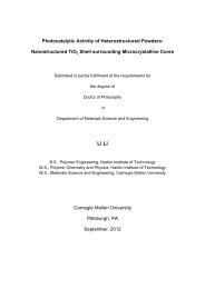
Taylor Model: Comparison to Polycrystal
The stress-strain curve
obtained for the
aggregate by Taylor in his
work is shown in the
figure. Although a
comparison of single
crystal (under multislip
conditions) and a
polycrystal is shown, it is
generally considered that
the good agreement
indicated by the lines was
somewhat fortuitous!
Note:
Circles - computed data
Crosses – experimental
data
The ratio between the two curves is the average Taylor factor, which in this case is ~3.1

€
67
Taylor’s Rigid Plastic Model for Polycrystals
Another important conclusion based on this calculation,
is that the overall stress-strain curve of the polycrystal is
given by the expression
σ = M τ(γ)
Where,
τ(γ) is the critical resolved shear stress (as a function of the resolved
shear strain) for a single crystal, assumed to have a single value;
is an average value of the Taylor factor of all the grains (which
changes with strain).
By Taylor’s calculation, for FCC polycrystal metals,
M = 3.1

68
For texture development it is necessary to obtain the
total spin for the aggregate. Note that the since all the
grains are assumed to be subjected to the same
displacement (or velocity field) as the aggregate, the
total rotation experienced by each grain will be the same
as that of the aggregate.
For uniaxial tension
Then,
Taylor Model: Grain Reorientation
W
=
W*
∑
α=1
=
dW e = −dW C = q (α ) dγ
(α )
Note: W e = W −W C
(α ) 1
qij =
2
0
ˆ
Note: “W”
denotes spin
here, not work
done
( (α ) (α ) (α )
b ˆ i n j b ˆ j n ) i
(α ) − ˆ

69
Taylor model: Reorientation: 1"
Review of effect of slip system activity:
Symmetric part of the distortion tensor
resulting from slip:
(s) 1
mij = b ˆ (s)
ˆ
(s)
i n j + b ˆ (s)
ˆ
(s)
j n i
Anti-symmetric part of Deformation Strain
Rate Tensor (used for calculating lattice
rotations, sum over active slip systems):
2
(s) 1
qij =
2
( )
( b ˆ (s) (s)
i n ˆ
j − b ˆ (s) (s) )
j n ˆ
i

70
Taylor model: Reorientation: 2"
Strain rate from slip (add up contributions
from all active slip systems):
D C = γ ˙ (s) m (s)
∑
s
Rotation rate from slip, W C , (add up
contributions from all active slip systems):
∑
s
W C = ˙ γ (s) q (s)

71
Taylor model: Reorientation: 3"
Rotation rate of crystal axes (W * ), where
we account for the rotation rate of the grain
itself, W g :
W * = W g − W C
Rate sensitive formulation for slip rate in
each crystal (solve as implicit equation for
stress):
( s )
D C = ˙
ε 0
Crystal axes grain slip
∑
s
m (s) :σ c
τ (s)
n
= τ (s)
( )
m (s) sgn m (s) :σ c

72
Taylor model: Reorientation: 4"
The shear strain rate
on each system is
also given by the
power-law relation
(once the stress is
determined):
˙ γ (s) = ˙ ε 0
= τ (s)
m (s) :σ c
τ (s)
n
( s )
sgn m (s) :σ c
= τ
( )
(s)

73
Iteration to determine stress
state in each grain"
An iterative procedure is required to find the solution
for the stress state, σ c , in each grain (at each step).
Once a solution is found, then individual slipping
rates (shear rates) can be calculated for each of the
s slip systems. The use of a rate sensitive
formulation for yield avoids the necessity of ad hoc
assumptions to resolve the ambiguity of slip system
selection.
Within the Lapp code, the relevant subroutines are
SSS and NEWTON

74
€
Update orientation: 1"
General formula for rotation matrix:
a ij = δ ij cosθ + e ijk n k sinθ
+ (1− cosθ)n in j
In the small angle limit (cosθ ~ 1, sinθ ~ θ):
a ij = δ ij + e ijk n k θ

75
Update orientation: 2"
In tensor form (small rotation approx.):
R = I + W*
General relations:
ω = 1/2 curl u = 1/2 curl{x-X}
- u := displacement
ω i = 1
2 e ijk∂u k /∂X j
Ω jk = −e ijkω i
ω i = −e ijkΩ jk

76
Update orientation: 3"
To rotate an orientation:
g new = R·g old
= (I + W*)·g old ,
or, if no “rigid body” spin (W g = 0),
g new ⎛⎛
= ⎜⎜ I + ˙
⎝⎝
∑
s
γ s q s
⎞⎞
⎟⎟ ⋅ g
⎠⎠
old
Note: more complex algorithm required for relaxed
constraints.

77
Combining small rotations"
It is useful to demonstrate that a set of small
rotations can be combined through addition
of the skew-symmetric parts, given that
rotations combine by (e.g.) matrix
multiplication.
This consideration reinforces the importance
of using small strain increments in simulation
of texture development.

78
Small Rotation Approximation"
R 3 = R 2 R 1
⇔ R 3 = I + ˙
γ 2q 2
⇔ R ik
γ 1q 1
( ) ( I + ˙ )
(3)
= δij + ˙ γ (2) ( (2)
q ) ij δ jk + ˙ γ (1) (1)
q jk
( )
(3)
⇔ Rik = δijδ
jk + δ ˙
ijγ (1) (1)
q jk + δ ˙
jkγ (2) (2)
qij + ˙ γ (2) (2)
q ˙
ij γ (1) (1)
q jk
(3)
≈ Rik = δ ik + γ ˙ (1) (1)
qik + γ ˙ (2) (2)
qik ⇔ R 3 = I +
Q.E.D.
∑
i
γ ˙ (i ) q (i)
Neglect this second
order term for
small rotations

79
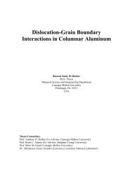
Taylor Model: Reorientation in Tension
Note that these results have been tested in considerable experimental detail by Winther et al. at Risø;
although Taylor’s results are correct in general terms, significant deviations are also observed*.
Texture development = mix of
and fibers
Initial configuration
Final configuration,
after 2.37% of extension
*Winther G., 2008, Slip systems, lattice rotations and dislocation boundaries, Materials Sci Eng. A483, 40-6
Each area within
the triangle
represents a
different operative
vertex on the
single crystal yield
surface

80
Taylor factor: multi-axial
stress and strain states"
The development given so far needs to be generalized for
arbitrary stress and strain states.
Write the deviatoric stress as the product of a tensor with
unit magnitude (in terms of von Mises equivalent stress) and
the (scalar) critical resolved shear stress, τ crss , where the
tensor defines the multiaxial stress state associated with a
particular strain direction, D.
S = M(D) τ crss .
Then we can find the (scalar) Taylor factor, M, by taking the
inner product of the stress deviator and the strain rate
tensor:
S:D = M(D):D τ crss = M τ crss .
See p 336 of [Kocks] and lecture 16E (RC model).

81
Summary"
Multiple slip is very different from single slip.
Multiaxial stress states are required to activate
multiple slip.
For cubic metals, there is a finite list of such
multiaxial stress states (56).
Minimum (microscopic) slip (Taylor) is equivalent
to maximum work (Bishop-Hill).
Solution of stress state still leaves the “ambiguity
problem” associated with the distribution of
(microscopic) slips; this is generally solved by
using a rate-sensitive solution.

82
Supplemental Slides"
Following slides contain information about a more
sophisticated model for crystal plasticity, called the
self-consistent model.
It is based on a finding a mean-field approximation
to the environment of each individual grain.
This provides the basis for the popular code VPSC
made available by Tomé and Lebensohn
(Lebensohn, R. A. and C. N. Tome (1993). "A Self-
Consistent Anisotropic Approach for the
Simulation of Plastic-Deformation and Texture
Development of Polycrystals - Application to
Zirconium Alloys." Acta Metallurgica et Materialia
41 2611-2624).

83
Kroner, Budiansky and Wu’s Model
Taylor’s Model
- compatibility across grain boundary
- violation of the equilibrium between the grains
Budiansky and Wu’s Model
- Self-consistent model
- ensure both compatibility and equilibrium
conditions on grain boundaries

84
The model:
Kroner, Budiansky and Wu’s Model
Sphere (single crystal grain)
embedded in a homogeneous
polycrystal matrix.
The grain and the matrix are
elastically isotropic.
Can be described by an elastic stiffness tensor C, which has
an inverse C -1 .
The matrix is considered to be infinitely extended.
σ*,ε
*
ε *
The overall quantities and are considered to be
p
the average values of the local quantities σ , ε and ε over all
randomly distributed single crystal grains.
p
Khan & Huang

85
Kroner, Budiansky and Wu’s Model
The initial problem can be solved by the following
approach
1 – split the proposed scheme into two other as follows
Khan & Huang

86
€
Kroner, Budiansky and Wu’s Model
1.a – The aggregate and grain are subject to the overall
quantities σ ,ε and ε . In this case the total strain
is given by the sum of the elastic and plastic strains:
p
€
€
ε = C -1 :σ +ε p
Khan & Huang

87
Kroner, Budiansky and Wu’s Model
1.b – The sphere
€
ε ʹ′ = ε p - ε p composite
has a stress-free transformation strain, ε’, which originates in the
difference in plastic response of the individual grain from the matrix as
a whole.
has the same elastic property as the aggregate
is very small when compared with the aggregate (the aggregate is
considered to extend to infinity)

88
Kroner, Budiansky and Wu’s Model
The strain inside the sphere due to the elastic interaction
between the grain and the aggregate caused by ε ʹ′ is given
by
ε = S : ε ʹ′ = S : (ε p - ε p )
Where,
S is the Eshelby
tensor (not a
compliance tensor)
for a sphere inclusion
in an isotropic elastic
matrix
€

€
89
Kroner, Budiansky and Wu’s Model
Then the actual strain inside the sphere is given by the sum
of the two representations (1a and 1b) as follows
Given that,
where
It leads to
€
ε = C -1 :σ +ε p + S : (ε p - ε p )
S : (ε p - ε p ) = β(ε p - ε p )
( 4 − 5ν
)
2
β =
15(
1−ν
)
ε = C :σ +ε p + β(ε p - ε p )

90
Kroner, Budiansky and Wu’s Model
From the previous equation, it follows that the stress inside
the sphere is given by
σ = C : ε
e
= C : ( ε − ε
p
)
= σ − 2G(1 − β)(ε p - ε p )
=

91
Kroner, Budiansky and Wu’s Model
In incremental form
where
σ ˙ = σ ˙ − 2G(1 − β)( ε ˙ p - ε ˙ p )
σ = (σ) ave , ˙
σ = ( ˙
σ ) ave
ε p = (ε p ) ave, ˙
ε p = ( ˙
ε p ) ave

92
Equations"
Slide 31: \tau = m_{11} \sigma_{11} + m_{22} \sigma_{22} + m_{33} \sigma_{33} + ( m_{12} + m_{21}) \sigma_{12} \\+ (m_{13} + m_
{31}) \sigma_{13} +(m_{23} + m_{32}) \sigma_{23}
SLIDE 34:
\begin{bmatrix} \tau_1& \\ \tau_2& \\ \tau_3& \\ \tau_4& \\ \tau_5& \end{bmatrix}= \begin{bmatrix} m_{11}^{(1) } & m_{22}^{(1) } & m_{33}^{(1)} & (m_{23}^{(1)}+m_{32}^{(1)}) & (m_
{13}^{(1)}+m_{31}^{(1)}) & (m_{12}^{(1)}+m_{21}^{(1)})
\\ m_{11}^{(2)} & m_{22}^{(2)} & m_{33}^{(2)} & (m_{23}^{(2)}+m_{32}^{(2)}) & (m_{13}^{(2)}+m_{31}^{(2)}) & (m_{12}^{(2)}+m_{21}^{(2)}) \\ m_{11}^{(3)} & m_{22}^{(3)} &
m_{33}^{(3)} & (m_{23}^{(3)}+m_{32}^{(3)}) & (m_{13}^{(3)}+m_{31}^{(3)}) & (m_{12}^{(3)}+m_{21}^{(3)}) \\
m_{11}^{(4)} & m_{22}^{(4)} & m_{33}^{(4)} & (m_{23}^{(4)}+m_{32}^{(4)}) & (m_{13}^{(4)}+m_{31}^{(4)}) & (m_{12}^{(4)}+m_{21}^{(4)}) \\
m_{11}^{(5)} & m_{22}^{(5)} & m_{33}^{(5)} & (m_{23}^{(5)}+m_{32}^{(5)}) & (m_{13}^{(5)}+m_{31}^{(5)}) & (m_{12}^{(5)}+m_{21}^{(5)}) \end{bmatrix}
\begin{bmatrix} \sigma_{11} \\ \sigma_{22} \\ \sigma_{33} \\ \sigma_{23} \\ \sigma_{13} \\ \sigma_{12} \end{bmatrix}
\begin{bmatrix} \tau_1& \\ \tau_2& \\ \tau_3& \\ \tau_4& \\ \tau_5& \end{bmatrix}= \begin{bmatrix} m_{22}^{(1) } & m_{33}^{(1)} & (m_{23}^{(1)}+m_{32}^{(1)}) & (m_{13}^{(1)}+m_{31}
^{(1)}) & (m_{12}^{(1)}+m_{21}^{(1)}) \\ m_{22}^{(2)} & m_{33}^{(2)} & (m_{23}^{(2)}+m_{32}^{(2)}) & (m_{13}^{(2)}+m_{31}^{(2)}) & (m_{12}^{(2)}+m_{21}^{(2)}) \\ m_{22}^
{(3)} & m_{33}^{(3)} & (m_{23}^{(1)}+m_{32}^{(3)}) & (m_{13}^{(3)}+m_{31}^{(3)}) & (m_{12}^{(3)}+m_{21}^{(3)}) \\
m_{22}^{(5)} & m_{33}^{(4)} & (m_{23}^{(1)}+m_{32}^{(4)}) & (m_{13}^{(4)}+m_{31}^{(4)}) & (m_{12}^{(4)}+m_{21}^{(4)}) \\
m_{22}^{(5)} & m_{33}^{(5)} & (m_{23}^{(5)}+m_{32}^{(5)}) & (m_{13}^{(5)}+m_{31}^{(5)}) & (m_{12}^{(5)}+m_{21}^{(5)}) \end{bmatrix}
\begin{bmatrix} -C \\ B \\ F \\ G \\ H \end{bmatrix}
\begin{bmatrix} -C \\ B \\ F \\ G \\ H \end{bmatrix} = \begin{bmatrix} m_{22}^{(1) } & m_{22}^{(2)} & m_{22}^{(3)} & m_{22}^{(4)} & m_{22}^{(5)} \\ m_{33}^{(1)} & m_{33}^{(2)}
& m_{33}^{(3)} & m_{33}^{(4)} & m_{33}^{(5)} \\ (m_{23}^{(1)}+m_{32}^{(1)}) & (m_{23}^{(2)}+m_{32}^{(2)}) & (m_{23}^{(3)}+m_{32}^{(3)}) & (m_{23}^{(4)}+m_{32}^{(4)})
& (m_{23}^{(5)}+m_{32}^{(5)}) \\ (m_{13}^{(1)}+m_{31}^{(1)}) & (m_{13}^{(2)}+m_{31}^{(2)}) & (m_{13}^{(3)}+m_{31}^{(3)}) & (m_{13}^{(4)}+m_{31}^{(4)}) & (m_{13}^{(5)}
+m_{31}^{(5)}) \\ (m_{12}^{(1)}+m_{21}^{(1)}) & (m_{12}^{(2)}+m_{21}^{(2)}) & (m_{12}^{(3)}+m_{21}^{(3)}) & (m_{12}^{(4)}+m_{21}^{(4)}) & (m_{12}^{(5)} +m_{21}^{(5)})
\end{bmatrix} \begin{bmatrix} \tau_1& \\ \tau_2& \\ \tau_3& \\ \tau_4& \\ \tau_5& \end{bmatrix}
SLIDE 37
\delta w = \sigma_{11} d\epsilon_{11} + \sigma_{22} d\epsilon_{22} +\sigma_{33} d\epsilon_{33} + 2 \sigma_{12} d\epsilon_{12} + 2 \sigma_{13} d\epsilon_{13} +
2 \sigma_{23} d\epsilon_{23}
SLIDE 53: \Omega_{ij}^{(\alpha)} = \frac{1}{2} (b_i&^{(\alpha)} n_j&^{(\alpha)} - b_j&^{(\alpha)} n_i&^{(\alpha)} )