Grain Boundary Properties: Energy (L21) - Materials Science and ...
Grain Boundary Properties: Energy (L21) - Materials Science and ...
Grain Boundary Properties: Energy (L21) - Materials Science and ...

You also want an ePaper? Increase the reach of your titles
YUMPU automatically turns print PDFs into web optimized ePapers that Google loves.
1<br />
Carnegie<br />
Mellon<br />
MRSEC<br />
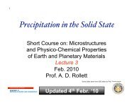
<strong>Grain</strong> <strong>Boundary</strong> <strong>Properties</strong>:<br />
<strong>Energy</strong> (<strong>L21</strong>)<br />
27-750, Fall 2009<br />
Texture, Microstructure & Anisotropy<br />
A.D. Rollett, P.N. Kalu<br />
With thanks to:<br />
G.S. Rohrer, D. Saylor,<br />
C.S. Kim, K. Barmak, others …<br />
Updated 19 th Nov. ‘09
2<br />
References<br />
• Interfaces in Crystalline <strong>Materials</strong>, Sutton & Balluffi, Oxford U.P.,<br />
1998. Very complete compendium on interfaces.<br />
• Interfaces in <strong>Materials</strong>, J. Howe, Wiley, 1999. Useful general text<br />
at the upper undergraduate/graduate level.<br />
• <strong>Grain</strong> <strong>Boundary</strong> Migration in Metals, G. Gottstein <strong>and</strong> L.<br />
Shvindlerman, CRC Press, 1999. The most complete review on<br />
grain boundary migration <strong>and</strong> mobility.<br />
• <strong>Materials</strong> Interfaces: Atomic-Level Structure & <strong>Properties</strong>, D. Wolf<br />
& S. Yip, Chapman & Hall, 1992.<br />
• See also mimp.materials.cmu.edu (Publications) for recent<br />
papers on grain boundary energy by researchers connected with<br />
the Mesoscale Interface Mapping Project (“MIMP”).
3<br />
Outline<br />
• Motivation, examples of anisotropic grain<br />
boundary properties<br />
• <strong>Grain</strong> boundary energy<br />
– Measurement methods<br />
– Surface Grooves<br />
– Low angle boundaries<br />
– High angle boundaries<br />
– <strong>Boundary</strong> plane vs. CSL<br />
– Herring relations, Young’s Law<br />
– Extraction of GB energy from dihedral angles<br />
– Capillarity Vector<br />
– Simulation of grain growth
4<br />
Why learn about grain boundary<br />
properties?<br />
• Many aspects of materials processing, properties <strong>and</strong><br />
performance are affected by grain boundary<br />
properties.<br />
• Examples include:<br />
- stress corrosion cracking in Pb battery electrodes,<br />
Ni-alloy nuclear fuel containment, steam generator<br />
tubes, aerospace aluminum alloys<br />
- creep strength in high service temperature alloys<br />
- weld cracking (under investigation)<br />
- electromigration resistance (interconnects)<br />
• <strong>Grain</strong> growth <strong>and</strong> recrystallization<br />
• Precipitation of second phases at grain boundaries<br />
depends on interface energy (& structure).
5<br />
<strong>Properties</strong>, phenomena of interest<br />
1. <strong>Energy</strong> (excess free energy → grain growth,<br />
coarsening, wetting, precipitation)<br />
2. Mobility (normal motion → grain growth,<br />
recrystallization)<br />
3. Sliding (tangential motion → creep)<br />
4. Cracking resistance (intergranular fracture)<br />
5. Segregation of impurities (embrittlement,<br />
formation of second phases)
6<br />
<strong>Grain</strong> <strong>Boundary</strong><br />
Diffusion<br />
• Especially for high symmetry<br />
boundaries, there is a very<br />
strong anisotropy of diffusion<br />
coefficients as a function of<br />
boundary type. This<br />
example is for Zn diffusing in<br />
a series of symmetric<br />
tilts in copper.<br />
• Note the low diffusion rates<br />
along low energy<br />
boundaries, especially Σ3.
7<br />
• <strong>Grain</strong> boundary sliding should<br />
be very structure dependent.<br />
Reasonable therefore that<br />
Biscondi’s results show that<br />
the rate at which boundaries<br />
slide is highly dependent on<br />
misorientation; in fact there is<br />
a threshold effect with no<br />
sliding below a certain<br />
misorientation at a given<br />
temperature.<br />
<strong>Grain</strong> <strong>Boundary</strong><br />
Sliding<br />
640°C<br />
600°C<br />
500°C<br />
Biscondi, M. <strong>and</strong> C. Goux (1968). "Fluage intergranulaire de<br />
bicristaux orientés d'aluminium." Mémoires Scientifiques Revue de Métallurgie 55(2): 167-179.
8<br />
<strong>Grain</strong> <strong>Boundary</strong> <strong>Energy</strong>: Definition<br />
• <strong>Grain</strong> boundary energy is defined as the excess free energy<br />
associated with the presence of a grain boundary, with the<br />
perfect lattice as the reference point.<br />
• A thought experiment provides a means of quantifying GB<br />
energy, γ. Take a patch of boundary with area A, <strong>and</strong> increase<br />
its area by dA. The grain boundary energy is the proportionality<br />
constant between the increment in total system energy <strong>and</strong> the<br />
increment in area. This we write:<br />
γ = dG/dA<br />
• The physical reason for the existence of a (positive) GB energy<br />
is misfit between atoms across the boundary. The deviation of<br />
atom positions from the perfect lattice leads to a higher energy<br />
state. Wolf established that GB energy is correlated with excess<br />
volume in an interface. There is no simple method, however, for<br />
predicting the excess volume.
9<br />
Measurement of GB <strong>Energy</strong><br />
• We need to be able to measure grain boundary<br />
energy.<br />
• In general, we do not need to know the absolute<br />
value of the energy but only how it varies with<br />
boundary type, i.e. with the crystallographic nature of<br />
the boundary.<br />
• For measurement of the anisotropy of the energy,<br />
then, we rely on local equilibrium at junctions<br />
between boundaries. This can be thought of as a<br />
force balance at the junctions.<br />
• For not too extreme anisotropies, the junctions<br />
always occur as triple lines.
10<br />
Experimental<br />
Methods for<br />
g.b. energy<br />
measurement<br />
G. Gottstein & L.<br />
Shvindlerman, <strong>Grain</strong><br />
<strong>Boundary</strong> Migration<br />
in Metals, CRC (1999)<br />
Method (a), with dihedral angles at triple lines, is most generally<br />
useful; method (c), with surface grooving also used.
11<br />
Zero-creep Method<br />
• The zero-creep experiment primarily measures the<br />
surface energy.<br />
• The surface energy tends to make a wire shrink so as<br />
to minimize its surface energy.<br />
• An external force (the weight) tends to elongate the<br />
wire.<br />
• Varying the weight can vary the extension rate from<br />
positive to negative, permitting the zero-creep point to<br />
be interpolated.<br />
• <strong>Grain</strong> boundaries perpendicular to the wire axis<br />
counteract the surface tension effect by tending to<br />
decrease the wire diameter.
12<br />
Herring Equations<br />
• We can demonstrate the effect of<br />
interfacial energies at the (triple)<br />
junctions of boundaries.<br />
• Equal g.b. energies on 3 GBs implies<br />
equal dihedral angles:<br />
1<br />
γ1 =γ2 =γ3 2 3<br />
120°
13<br />
Definition of Dihedral Angle<br />
• Dihedral angle, χ:= angle between the<br />
tangents to an adjacent pair of<br />
boundaries (unsigned). In a triple<br />
junction, the dihedral angle is assigned<br />
to the opposing boundary.<br />
1<br />
2 3<br />
120°<br />
γ 1 =γ 2 =γ 3<br />
χ 1 : dihedral<br />
angle for g.b.1
14<br />
Dihedral Angles<br />
• An material with uniform grain boundary energy should have<br />
dihedral angles equal to 120°.<br />
• Likely in real materials? No! Low angle boundaries (crystalline<br />
materials) always have a dislocation structure <strong>and</strong> therefore a<br />
monotonic increase in energy with misorientation angle (Read-<br />
Shockley model).<br />
• The inset figure is taken from a paper in preparation by Prof. K.<br />
Barmak <strong>and</strong> shows the distribution of dihedral angles measured<br />
in a 0.1 µm thick film of Al, along with a calculated distribution<br />
based on an GB energy function from a similar film (with two<br />
different assumptions about the distribution of misorientations).
15<br />
Unequal energies<br />
• If the interfacial energies are not equal, then<br />
the dihedral angles change. A low g.b. energy<br />
on boundary 1 increases the corresponding<br />
dihedral angle.<br />
1<br />
2 3<br />
χ 1>120°<br />
γ 1
16<br />
Unequal Energies, contd.<br />
• A high g.b. energy on boundary 1 decreases<br />
the corresponding dihedral angle.<br />
• Note that the dihedral angles depend on all<br />
the energies.<br />
2<br />
1<br />
3<br />
χ1< 120°<br />
γ 1 >γ 2 =γ 3
17<br />
Wetting<br />
• For a large enough ratio, wetting can<br />
occur, i.e. replacement of one boundary<br />
by the other two at the TJ.<br />
γ 2 cosχ 1 /2<br />
2<br />
γ 1<br />
1<br />
3<br />
χ1< 120°<br />
γ 3 cosχ 1 /2<br />
γ 1 >γ 2 =γ 3<br />
Balance vertical<br />
forces ⇒<br />
γ 1 = 2γ 2 cos(χ 1 /2)<br />
Wetting ⇒<br />
γ 1 ≥ 2 γ 2
18<br />
Triple Junction Quantities<br />
g A<br />
^<br />
b 1<br />
χ<br />
^<br />
n 3<br />
2<br />
n ^<br />
1<br />
χ 3<br />
^<br />
b3 χ 1<br />
φ 2<br />
g B<br />
^<br />
n 2<br />
g C<br />
^<br />
b 2
19<br />
Triple Junction Quantities<br />
• <strong>Grain</strong> boundary tangent (at a TJ): b<br />
• <strong>Grain</strong> boundary normal (at a TJ): n<br />
• <strong>Grain</strong> boundary inclination, measured anticlockwise<br />
with respect to a(n arbitrarily<br />
chosen) reference direction (at a TJ): φ<br />
• <strong>Grain</strong> boundary dihedral angle: χ<br />
• <strong>Grain</strong> orientation:g
20<br />
Force Balance Equations/<br />
Herring Equations<br />
• The Herring equations[(1951). Surface tension as a motivation<br />
for sintering. The Physics of Powder Metallurgy. New York,<br />
McGraw-Hill Book Co.: 143-179] are force balance equations at<br />
a TJ. They rely on a local equilibrium in terms of free energy.<br />
• A virtual displacement, δr, of the TJ (L in the figure) results in no<br />
change in free energy.<br />
• See also: Kinderlehrer D <strong>and</strong> Liu C, Mathematical Models <strong>and</strong><br />
Methods in Applied <strong>Science</strong>s, (2001) 11 713-729; Kinderlehrer,<br />
D., Lee, J., Livshits, I., <strong>and</strong> Ta'asan, S. (2004) Mesoscale<br />
simulation of grain growth, in Continuum Scale Simulation of<br />
Engineering <strong>Materials</strong>, (Raabe, D. et al., eds),Wiley-VCH<br />
Verlag, Weinheim, Chap. 16, 361-372
21<br />
Derivation of Herring Equs.<br />
A virtual displacement, δr, of the TJ results in<br />
no change in free energy.<br />
See also: Kinderlehrer, D <strong>and</strong> Liu, C Mathematical Models <strong>and</strong> Methods in Applied <strong>Science</strong>s {2001} 11<br />
713-729; Kinderlehrer, D., Lee, J., Livshits, I., <strong>and</strong> Ta'asan, S. 2004 Mesoscale simulation of grain<br />
growth, in Continuum Scale Simulation of Engineering <strong>Materials</strong>, (Raabe, D. et al., eds), Wiley-VCH<br />
Verlag, Weinheim, Chapt. 16, 361-372
22<br />
Force Balance<br />
• Consider only interfacial energy: vector<br />
sum of the forces must be zero to<br />
satisfy equilibrium.<br />
• These equations can be rearranged to<br />
give the Young equations (sine law):<br />
€<br />
γ 1<br />
sin χ 1<br />
γ 1b 1 +γ 2b 2 +γ 3b 3 = <br />
0<br />
= γ 2<br />
sin χ 2<br />
= γ 3<br />
sin χ 3
23<br />
γ S2<br />
Analysis of Thermal Grooves<br />
γ Gb<br />
Surface 2<br />
γ S1<br />
d<br />
Crystal 1<br />
W<br />
2W<br />
Ψs It is often reasonable to assume a constant surface energy, γ S , <strong>and</strong> examine the<br />
variation in GB energy, γ Gb , as it affects the thermal groove angles<br />
?<br />
β<br />
Surface<br />
Crystal 2
<strong>Grain</strong> <strong>Boundary</strong> <strong>Energy</strong> Distribution is<br />
Affected by Composition<br />
Δγ = 1.09<br />
Δγ = 0.46<br />
1 µm<br />
Ca solute increases the range of the γ GB /γ S ratio. The variation of the relative energy in<br />
undoped MgO is lower (narrower distribution) than in the case of doped material.<br />
76
Bi impurities in Ni have the opposite effect<br />
Pure Ni, grain size:<br />
20µm<br />
Bi-doped Ni, grain size:<br />
21µm<br />
Range of γ GB /γ S (on log scale) is smaller for Bi-doped Ni than for pure Ni,<br />
indicating smaller anisotropy of γ GB /γ S . This correlates with the plane distribution<br />
77
26<br />
G.B. <strong>Properties</strong> Overview: <strong>Energy</strong><br />
• Low angle boundaries can be<br />
treated as dislocation structures,<br />
as analyzed by Read & Shockley<br />
(1951).<br />
• <strong>Grain</strong> boundary energy can be<br />
constructed as the average of<br />
the two surface energies -<br />
γ GB = γ(hkl A )+γ(hkl B ).<br />
• For example, in fcc metals, low<br />
energy boundaries are found<br />
with {111} terminating surfaces.<br />
• Does mobility scale with g.b.<br />
energy, based on a dependence<br />
on acceptor/donor sites?<br />
Read-Shockley<br />
one {111}<br />
Shockley W, Read WT. Quantitative Predictions From Dislocation<br />
Models Of Crystal <strong>Grain</strong> Boundaries. Phys. Rev. 1949;75:692."<br />
two {111}<br />
planes (Σ3 …)
27<br />
<strong>Grain</strong> boundary energy: current status?<br />
• Limited information available:<br />
– Deep cusps exist for a few CSL types in fcc (Σ3, Σ11), based<br />
on both experiments <strong>and</strong> simulation.<br />
– Extensive simulation results [Wolf et al.] indicate that interfacial free<br />
volume is good predictor. No simple rules available, however, to<br />
predict free volume.<br />
– Wetting results in iron [Takashima, Wynblatt] suggest that a broken<br />
bond approach (with free volume <strong>and</strong> twist angle) provides a<br />
reasonable 5-parameter model.<br />
– If binding energy is neglected, an average of the surface energies is<br />
a good predictor of grain boundary energy in MgO [Saylor, Rohrer].<br />
– Minimum dislocation density structures [Frank - see description in<br />
Sutton & Balluffi] provide a good model of g.b. energy in MgO, <strong>and</strong><br />
may provide a good model of low angle grain boundary mobility.
28<br />
<strong>Grain</strong> <strong>Boundary</strong> <strong>Energy</strong><br />
• First categorization of boundary type is into low-angle<br />
versus high-angle boundaries. Typical value in cubic<br />
materials is 15° for the misorientation angle.<br />
• Typical values of g.b. energies vary from<br />
0.32 J.m -2 for Al to 0.87 for Ni J.m -2 (related to bond<br />
strength, which is related to melting point).<br />
• Read-Shockley model describes the energy variation<br />
with angle for low-angle boundaries successfully in<br />
many experimental cases, based on a dislocation<br />
structure.
29<br />
Read-Shockley model<br />
• Start with a symmetric tilt boundary<br />
composed of a wall of infinitely straight,<br />
parallel edge dislocations (e.g. based<br />
on a 100, 111 or 110 rotation axis with<br />
the planes symmetrically disposed).<br />
• Dislocation density (L -1 ) given by:<br />
1/D = 2sin(θ/2)/b ≈ θ/b for small<br />
angles.
30<br />
Tilt boundary<br />
Each dislocation accommodates the mismatch between the two lattices; for<br />
a or misorientation axis in the boundary plane, only one type of<br />
dislocation (a single Burgers vector) is required.<br />
b<br />
D
31<br />
Read-Shockley contd.<br />
• For an infinite array of edge dislocations the longrange<br />
stress field depends on the spacing. Therefore<br />
given the dislocation density <strong>and</strong> the core energy of<br />
the dislocations, the energy of the wall (boundary) is<br />
estimated (r 0 sets the core energy of the dislocation):<br />
γ gb = E 0 θ(A 0 - lnθ), where<br />
E 0 = µb/4π(1-ν); A 0 = 1 + ln(b/2πr 0 )
32<br />
LAGB experimental results<br />
• Experimental results on copper. Note the<br />
lack of evidence of deep minima (cusps) in<br />
energy at CSL boundary types in the <br />
tilt or twist boundaries.<br />
Disordered Structure<br />
Dislocation Structure<br />
[Gjostein & Rhines, Acta metall. 7, 319 (1959)]
33<br />
Read-Shockley contd.<br />
• If the non-linear form for the dislocation<br />
spacing is used, we obtain a sine-law<br />
variation (U core = core energy):<br />
γ gb = sin|θ| {U core /b - µb 2 /4π(1-ν) ln(sin|θ|)}<br />
• Note: this form of energy variation may also<br />
be applied to CSL-vicinal boundaries.
34<br />
<strong>Energy</strong> of High Angle Boundaries<br />
• No universal theory exists to describe the energy of HAGBs.<br />
• Based on a disordered atomic structure for general high angle<br />
boundaries, we expect that the g.b. energy should be at a<br />
maximum <strong>and</strong> approximately constant.<br />
• Abundant experimental evidence for special boundaries at (a<br />
small number) of certain orientations for which the atomic fit is<br />
better than in general high angle g.b’s.<br />
• Each special point (in misorientation space) expected to have a<br />
cusp in energy, similar to zero-boundary case but with non-zero<br />
energy at the bottom of the cusp.<br />
• Atomistic simulations suggest that g.b. energy is (positively)<br />
correlated with free volume at the interface.
35<br />
Exptl. vs. Computed E gb<br />
<br />
Tilts<br />
Σ11 with (311) plane<br />
<br />
Tilts<br />
Σ3, 111 plane: CoherentTwin<br />
Note the<br />
presence of<br />
local minima<br />
in the <br />
series, but<br />
not in the<br />
<br />
series of tilt<br />
boundaries.<br />
Hasson & Goux, Scripta metall. 5 889-94
36<br />
Surface Energies vs.<br />
<strong>Grain</strong> <strong>Boundary</strong> <strong>Energy</strong><br />
• A recently revived, but still controversial idea, is that the grain<br />
boundary energy is largely determined by the energy of the two<br />
surfaces that make up the boundary (<strong>and</strong> that the twist angle is<br />
not significant).<br />
• This is has been demonstrated to be highly accurate in the case<br />
of MgO, which is an ionic ceramic with a rock-salt structure. In<br />
this case, {100} has the lowest surface energy, so boundaries<br />
with a {100} plane are expected to be low energy.<br />
• The next slide, taken from the PhD thesis work of David Saylor,<br />
shows a comparison of the g.b. energy computed as the<br />
average of the two surface energies, compared to the frequency<br />
of boundaries of the corresponding type. As predicted, the<br />
frequency is lowest for the highest energy boundaries, <strong>and</strong> vice<br />
versa.
37<br />
2<br />
i<br />
i+2<br />
r ij1<br />
l’ ij<br />
j<br />
1<br />
j<br />
3<br />
r ij2<br />
n’ ij<br />
i+1<br />
• Index n’ in the crystal<br />
reference frame:<br />
n = g i n' <strong>and</strong> n = g i+1 n'<br />
(2 parameter description)<br />
λ(n)<br />
(MRD)
38<br />
g A<br />
θ<br />
Lattice Misorientation, ∆g (rotation, 3 parameters)<br />
<strong>Boundary</strong> Plane Normal, n (unit vector, 2 parameters)<br />
g B<br />
<strong>Grain</strong> Boundaries have 5 Macroscopic Degrees of Freedom
39<br />
Tilt versus Twist Boundaries<br />
Isolated/occluded grain (one grain enclosed within another)<br />
illustrates variation in boundary plane for constant misorientation.<br />
The normal is // misorientation axis for a twist boundary whereas<br />
for a tilt boundary, the normal is ⊥ to the misorientation axis. Many<br />
variations are possible for any given boundary.<br />
Misorientation axis<br />
Twist boundaries
40<br />
l=100<br />
(√2-1,0)<br />
l=111<br />
Separation of ∆g <strong>and</strong> n<br />
Plotting the boundary plane requires a full hemisphere which<br />
projects as a circle. Each projection describes the variation at<br />
fixed misorientation. Any (numerically) convenient discretization<br />
of misorientation <strong>and</strong> boundary plane space can be used.<br />
(√2-1,√2-1)<br />
l=110<br />
R1+R2+R3=1<br />
Misorientation axis, e.g. 111,<br />
also the twist type location<br />
Distribution of normals<br />
for boundaries with Σ3<br />
misorientation<br />
(commercial purity Al)
41<br />
λ(Δg, n)<br />
λ(n|5°/[100])<br />
λ(n|15°/[100])<br />
λ(n|25°/[100])<br />
λ(n|35°/[100])<br />
n^ [100]<br />
n^<br />
n^<br />
n^<br />
n^<br />
n^<br />
n^<br />
n^<br />
Every peak in λ(Δg,n) is related to a boundary with a {100} plane
42<br />
MgO<br />
SrTiO 3<br />
<strong>Grain</strong> <strong>Boundary</strong><br />
Population (Δg averaged)<br />
Measured Surface<br />
Energies<br />
Saylor & Rohrer, Inter. Sci. 9 (2001) 35.<br />
Sano et al., J. Amer. Ceram. Soc., 86 (2003) 1933.
43<br />
For all grain boundaries in MgO<br />
ln(λ+1)<br />
3.0<br />
2.5<br />
2.0<br />
1.5<br />
1.0<br />
0.5<br />
0.0<br />
0.70 0.78 0.86 0.94 1.02<br />
γ gb (a.u)<br />
Saylor DM, Morawiec A, Rohrer GS. Distribution <strong>and</strong> Energies of <strong>Grain</strong> Boundaries as a Function of Five Degrees<br />
of Freedom. Journal of The American Ceramic Society 2002;85:3081. Capillarity vector used to calculate the grain<br />
boundary energy distribution – see later slides.
44<br />
[100] misorientations in MgO<br />
<strong>Grain</strong> boundary<br />
energy<br />
γ(n|ω/[100])<br />
<strong>Grain</strong> boundary<br />
distribution<br />
λ(n|ω/[100])<br />
ω= 10° ω= 30°<br />
ω=10°<br />
Population <strong>and</strong> <strong>Energy</strong> are inversely correlated<br />
Saylor, Morawiec, Rohrer, Acta Mater. 51 (2003) 3675<br />
MRD<br />
ω= 30°<br />
MRD
45<br />
Symmetric [110]<br />
tilt boundaries<br />
<strong>Energy</strong>, a.u.<br />
0.8<br />
0.6<br />
0.4<br />
Σ= 9 11 3 3 11 9<br />
Energies:<br />
G.C. Hasson <strong>and</strong> C. Goux<br />
0.2<br />
5<br />
Scripta Met. 5 (1971) 889.<br />
0<br />
0<br />
Al boundary populations:<br />
Saylor et al. Acta mater., 52, 3649-3655 (2004).<br />
30 60 90 120 150<br />
Misorientation angle, deg.<br />
0<br />
180<br />
30<br />
25<br />
20<br />
15<br />
10<br />
λ(Δg, n), MRD
46<br />
λ<br />
γ<br />
γ gb (a.u)<br />
0.91<br />
0.90<br />
0.89<br />
0.88<br />
0.87<br />
(031)<br />
(031)<br />
(043)<br />
(010)<br />
(012)<br />
(021)<br />
(001)<br />
(034)<br />
(013)<br />
(013)<br />
0 30 60 90 120 150 180 0.30<br />
θ 010 (°)<br />
(034)<br />
(001)<br />
(021)<br />
(012)<br />
The energy-population correlation is not one-to-one<br />
0.55<br />
0.50<br />
0.45<br />
0.40<br />
0.35<br />
λ (MRD)
47<br />
Inclination Dependence<br />
• Interfacial energy can depend on inclination,<br />
i.e. which crystallographic plane is involved.<br />
• Example? The coherent twin boundary is<br />
obviously low energy as compared to the<br />
incoherent twin boundary (e.g. Cu, Ag). The<br />
misorientation (60° about ) is the same,<br />
so inclination is the only difference.
48<br />
Twin: coherent vs. incoherent<br />
• Porter &<br />
Easterling<br />
fig. 3.12/<br />
p123
49<br />
The torque term<br />
Change in inclination causes a change in its energy,<br />
tending to twist it (either back or forwards)<br />
dφ<br />
ˆ<br />
n 1
50<br />
Inclination Dependence, contd.<br />
• For local equilibrium at a TJ, what matters is<br />
the rate of change of energy with inclination,<br />
i.e. the torque on the boundary.<br />
• Recall that the virtual displacement twists<br />
each boundary, i.e. changes its inclination.<br />
• Re-express the force balance as (σ≡γ):<br />
surface<br />
tension<br />
terms<br />
σ j ˆ<br />
3<br />
{ ∑ b j + ∂σ j ∂φ j<br />
j = 1<br />
( ) ˆ<br />
n j} = torque terms<br />
0
51<br />
Herring’s Relations
52<br />
Torque effects<br />
• The effect of inclination seems esoteric: should<br />
one be concerned about it?<br />
• Yes! Twin boundaries are only one example<br />
where inclination has an obvious effect. Other<br />
types of grain boundary (to be explored later)<br />
also have low energies at unique<br />
misorientations.<br />
• Torque effects can result in inequalities*<br />
instead of equalities for dihedral angles, if one<br />
of the boundaries is in a cusp, such as for the<br />
coherent twin.<br />
* B.L. Adams, et al. (1999). “Extracting <strong>Grain</strong> <strong>Boundary</strong> <strong>and</strong> Surface <strong>Energy</strong> from Measurement of Triple Junction <br />
Geometry.” Interface <strong>Science</strong> 7: 321-337."
53<br />
Aluminum foil, cross section<br />
• Torque term<br />
literally twists<br />
the boundary<br />
away from<br />
being<br />
perpendicular<br />
to the surface<br />
θ L<br />
θ S<br />
surface<br />
Cross-section of<br />
a thin foil of Al.
54<br />
Why Triple Junctions?<br />
• For isotropic g.b. energy, 4-fold junctions split<br />
into two 3-fold junctions with a reduction in<br />
free energy:<br />
90°<br />
120°
55<br />
How to Measure Dihedral<br />
Angles <strong>and</strong> Curvatures: 2D microstructures<br />
(1)<br />
Image<br />
Processing<br />
(2) Fit conic sections to each grain boundary:<br />
Q(x,y)=Ax 2 + Bxy+ Cy 2 + Dx+<br />
Ey+F = 0<br />
Assume a quadratic curve is adequate to describe the shape<br />
of a grain boundary. [PhD thesis, CMU, CC Yang 2001]
56<br />
(3) Calculate the tangent angle <strong>and</strong> curvature at a triple<br />
junction from the fitted conic function, Q(x,y):<br />
y ʹ′ = dy<br />
dx<br />
= −(2Ax + By + D)<br />
Bx + 2Cy + E<br />
y ʹ′ = d 2 y<br />
dx 2 = −(2A + 2By ʹ′ + 2Cy ʹ′<br />
2 )<br />
2Cy + Bx + E<br />
κ =<br />
y ʹ′<br />
(1+ y ʹ′<br />
2 )<br />
3<br />
2<br />
; θ tan = tan −1<br />
y<br />
ʹ′<br />
Q(x,y)=Ax 2 + Bxy<br />
+ Cy 2 + Dx+<br />
Ey+F=0
57<br />
Calculation of G.B. <strong>Energy</strong><br />
• In principle, one can measure many different triple junctions to<br />
characterize crystallography, dihedral angles <strong>and</strong> curvature.<br />
• From these measurements one can extract the relative<br />
properties of the grain boundaries.<br />
• The simpler procedure, described here, uses the dihedral<br />
angles <strong>and</strong> calculates the GB energy based on the 3<br />
parameters of misorientation only, i.e. neglecting the torque<br />
term.<br />
• The more complete calculation of GB energy is performed for all<br />
5 macroscopic degrees of freedom. Since this does include the<br />
torque term, the capillarity vector can be used to accomplish<br />
this. The concept of the capillarity vector is described in<br />
subsequent slides.
58<br />
Measurements at<br />
many TJs; bin the<br />
<strong>Energy</strong> Extraction<br />
(sinχ 2 ) σ 1 - (sinχ 1 ) σ 2 = 0<br />
(sinχ 3 ) σ 2 - (sinχ 2 ) σ 3 = 0<br />
sinχ 2 -sinχ 1 0 0 …0<br />
0 sinχ 3 -sinχ 2 0 ...0<br />
* * 0 0 ...0<br />
: : : : :<br />
0 0 * * 0<br />
dihedral angles by g.b. type; average the sinχ i ;<br />
each TJ gives a pair of equations<br />
• PhD thesis, CMU, CC Yang 2001.<br />
• D. Kinderlehrer, et al. , Proc. of the Twelfth International Conference on Textures of <strong>Materials</strong>, Montréal, Canada, (1999) 1643.<br />
• K. Barmak, et al., "<strong>Grain</strong> boundary energy <strong>and</strong> grain growth in Al films: Comparison of experiments <strong>and</strong> simulations", Scripta<br />
materialia, 54 (2006) 1059-1063: following slides …<br />
σ 1<br />
σ 2<br />
σ 3<br />
:<br />
σ n<br />
= 0
60<br />
3<br />
⎪⎪⎧⎧<br />
∑ ⎨⎨σ<br />
ˆ<br />
jb<br />
j<br />
j=<br />
1 ⎪⎪⎩⎩<br />
⎡⎡∂σ<br />
⎤⎤ ⎪⎪⎫⎫<br />
<br />
j<br />
+ ⎢⎢ ⎥⎥nˆ<br />
j ⎬⎬ = 0<br />
⎢⎢⎣⎣<br />
∂φ<br />
j ⎥⎥⎦⎦<br />
⎪⎪⎭⎭<br />
σ 1 σ 2 =<br />
sin χ sin χ<br />
σ 3 =<br />
sin χ<br />
1<br />
Equilibrium at Triple Junctions<br />
b j - boundary tangent<br />
n j - boundary normal<br />
χ - dihedral angle<br />
σ - grain boundary energy<br />
Since the crystals have strong {111} fiber<br />
texture, we assume ;<br />
- all grain boundaries are pure {111} tilt<br />
boundaries<br />
- the tilt angle is the same as the<br />
misorientation angle<br />
K. Barmak, et al.<br />
2<br />
3<br />
Herring’s Eq.<br />
Young’s Eq.<br />
Example: {001} c [001] s textured Al foil<br />
To measure lines, triple junctions <strong>and</strong><br />
dihedral angles, one can use Linefollow<br />
(S. Mahadevan <strong>and</strong> D. Casasent: Proc.<br />
SPIE, 2001, pp 204-214.)
61<br />
3 µm<br />
Al film<br />
[001] sample<br />
K. Barmak, et al.<br />
Cross-Sections Using OIM<br />
SEM image<br />
[010] sample<br />
[001] inverse pole figure map, raw data<br />
[001] inverse pole figure map, cropped cleaned data<br />
- remove Cu (~0.1 mm)<br />
- clean up using a grain dilation method (min. pixel 10)<br />
[010] inverse pole figure map, cropped cleaned data<br />
scanned cross-section<br />
more examples<br />
3 µm
62<br />
<strong>Grain</strong> <strong>Boundary</strong> <strong>Energy</strong> Calculation : Method<br />
Type 2<br />
Young’s Equation<br />
σ 1 σ 2 σ 3<br />
= =<br />
sin χ sin χ sin χ<br />
1<br />
K. Barmak, et al.<br />
Type 1<br />
2<br />
χ 2<br />
3<br />
Type 3<br />
σ<br />
1<br />
2<br />
1<br />
Type 1 - Type 2 = Type 2 - Type 1<br />
Type 2 - Type 3 = Type 3 - Type 2<br />
Type 1 - Type 3 = Type 3 - Type 1<br />
Pair boundaries <strong>and</strong> put<br />
into urns of pairs<br />
Linear, homogeneous equations<br />
σ sin χ<br />
2<br />
sin χ<br />
3<br />
3<br />
−σ<br />
−σ<br />
2<br />
3<br />
3<br />
sin χ<br />
sin χ<br />
σ sin χ −σ<br />
sin χ<br />
1<br />
1<br />
2<br />
=<br />
=<br />
=<br />
0<br />
0<br />
0
63<br />
<strong>Grain</strong> <strong>Boundary</strong> <strong>Energy</strong> Calculation : Method<br />
N×(N-1)/2 equations<br />
N unknowns i<br />
N<br />
j<br />
j<br />
ij<br />
b<br />
A =<br />
∑ =1<br />
γ i=1,….,N(N-1)/2<br />
⎥⎥<br />
⎥⎥<br />
⎥⎥<br />
⎥⎥<br />
⎥⎥<br />
⎥⎥<br />
⎥⎥<br />
⎥⎥<br />
⎥⎥<br />
⎥⎥<br />
⎥⎥<br />
⎦⎦<br />
⎤⎤<br />
⎢⎢<br />
⎢⎢<br />
⎢⎢<br />
⎢⎢<br />
⎢⎢<br />
⎢⎢<br />
⎢⎢<br />
⎢⎢<br />
⎢⎢<br />
⎢⎢<br />
⎢⎢<br />
⎣⎣<br />
⎡⎡<br />
=<br />
⎥⎥<br />
⎥⎥<br />
⎥⎥<br />
⎥⎥<br />
⎥⎥<br />
⎥⎥<br />
⎦⎦<br />
⎤⎤<br />
⎢⎢<br />
⎢⎢<br />
⎢⎢<br />
⎢⎢<br />
⎢⎢<br />
⎢⎢<br />
⎣⎣<br />
⎡⎡<br />
⎥⎥<br />
⎥⎥<br />
⎥⎥<br />
⎥⎥<br />
⎥⎥<br />
⎥⎥<br />
⎥⎥<br />
⎥⎥<br />
⎥⎥<br />
⎥⎥<br />
⎥⎥<br />
⎦⎦<br />
⎤⎤<br />
⎢⎢<br />
⎢⎢<br />
⎢⎢<br />
⎢⎢<br />
⎢⎢<br />
⎢⎢<br />
⎢⎢<br />
⎢⎢<br />
⎢⎢<br />
⎢⎢<br />
⎢⎢<br />
⎣⎣<br />
⎡⎡<br />
−<br />
−<br />
−<br />
−<br />
−<br />
−<br />
−<br />
0<br />
0<br />
0<br />
0<br />
0<br />
0<br />
0<br />
sin<br />
sin<br />
0<br />
0<br />
0<br />
0<br />
0<br />
0<br />
0<br />
0<br />
0<br />
0<br />
0<br />
0<br />
0<br />
sin<br />
0<br />
sin<br />
0<br />
0<br />
0<br />
0<br />
0<br />
0<br />
0<br />
sin<br />
sin<br />
0<br />
0<br />
0<br />
0<br />
0<br />
0<br />
0<br />
sin<br />
0<br />
0<br />
sin<br />
0<br />
0<br />
0<br />
0<br />
0<br />
0<br />
sin<br />
0<br />
sin<br />
0<br />
0<br />
0<br />
0<br />
0<br />
0<br />
0<br />
sin<br />
sin<br />
3<br />
2<br />
1<br />
1<br />
2<br />
4<br />
2<br />
3<br />
1<br />
4<br />
1<br />
3<br />
1<br />
2<br />
<br />
<br />
<br />
<br />
<br />
<br />
<br />
<br />
<br />
<br />
<br />
<br />
<br />
<br />
<br />
<br />
<br />
<br />
<br />
<br />
<br />
<br />
<br />
<br />
<br />
<br />
N<br />
N<br />
N<br />
γ<br />
γ<br />
γ<br />
γ<br />
ϕ<br />
ϕ<br />
ϕ<br />
ϕ<br />
ϕ<br />
ϕ<br />
ϕ<br />
ϕ<br />
ϕ<br />
ϕ<br />
ϕ<br />
ϕ<br />
N(N-1)/2<br />
N<br />
=<br />
N<br />
N(N-1)/2<br />
K. Barmak, et al.
64<br />
# of total TJs : 8694<br />
# of {111} TJs : 7367 (10° resolution)<br />
22101 (=7367×3) boundaries<br />
2° binning<br />
(0°-1°, 1° -3°, 3° -5°, …,59° -61°,61° -62°)<br />
32×31/2=496 pairs<br />
no data at low angle boundaries (
65<br />
Tilt Boundaries: Results<br />
Relative <strong>Boundary</strong> <strong>Energy</strong><br />
1 2 .<br />
1 0 .<br />
0 8 .<br />
0 6 .<br />
Σ13<br />
1 0 2 0 3 0 4 0 5 0 6 0<br />
M i s o r i e n t a t i o n A n g l e , o<br />
• Cusps at tilt angles of 28 <strong>and</strong> 38 degrees, corresponding to CSL type<br />
boundaries Σ13 <strong>and</strong> Σ7, respectively.<br />
• Remember that boundaries in a strongly textured thin film are<br />
constrained to be 111 tilt boundaries.<br />
K. Barmak, et al.<br />
Σ7
66<br />
Capillarity Vector<br />
• The capillarity vector is a convenient quantity to use in<br />
force balances at junctions of surfaces.<br />
• It is derived from the variation in (excess free) energy<br />
of a surface.<br />
• In effect, the capillarity vector combines both the<br />
surface tension (so-called) <strong>and</strong> the torque terms into a<br />
single vector quantity.<br />
• The vector sum of the capillarity vectors of three<br />
boundaries joined at a triple line must (vector) sum to<br />
zero, or, more precisely, the vector sum cross the line<br />
tangent must be zero.<br />
• It is therefore feasible to construct an algorithm that<br />
computes the anisotropy of grain boundary energy<br />
based on (iteratively) minimizing the error of the<br />
above vector sum at all triple lines.
67<br />
Equilibrium at TJ<br />
• The utility of the capillarity vector, ξ, can be illustrated by rewriting<br />
Herring’s equations as follows, where l 123 is the triple line<br />
(tangent) vector.<br />
(ξ 1 + ξ 2 + ξ 3 ) x l 123 = 0<br />
• Note that the cross product with the triple line tangent implies<br />
resolution of forces perpendicular to the triple line.<br />
• Used by the MIMP group to calculate the GB energy function for<br />
MgO, based on a dataset with boundary normals (which imply<br />
dihedral angles) <strong>and</strong> grain orientations:<br />
Morawiec A. Method to calculate the grain boundary energy<br />
distribution over the space of macroscopic boundary parameters from<br />
the geometry of triple junctions. Acta mater. 2000;48:3525.<br />
Also, Saylor DM, Morawiec A, Rohrer GS. Distribution <strong>and</strong> Energies<br />
of <strong>Grain</strong> Boundaries as a Function of Five Degrees of Freedom.<br />
Journal of The American Ceramic Society 2002;85:3081."
68<br />
Capillarity vector definition<br />
• Following Hoffman & Cahn, define a unit<br />
surface normal vector to the surface, n<br />
ˆ , <strong>and</strong><br />
a scalar field, rγ( n ˆ ), where r is a radius from<br />
the origin. Typically, the normal is defined<br />
w.r.t. crystal axes.<br />
• “A vector thermodynamics for anisotropic<br />
surfaces. I. Fundamentals <strong>and</strong> application to<br />
plane surface junctions.”, D.W. Hoffman <strong>and</strong><br />
J.W. Cahn, Surface <strong>Science</strong> 31: 368-388<br />
(1972). Also read sections 5.6.4 & 5.6.5 in<br />
Sutton & Balluffi."
69<br />
Capillarity vector: derivations<br />
• Definition:<br />
• From which, Eq (1)<br />
• Giving,<br />
• Compare with the<br />
rule for products:<br />
gives: (2), <strong>and</strong>, (3)<br />
• Combining total derivative of (2), with (3):<br />
Eq (4):
71<br />
Computer Simulation of<br />
<strong>Grain</strong> Growth<br />
• From the PhD thesis project of Jason Gruber.<br />
• MgO-like grain boundary properties were<br />
incorporated into a finite element model of grain<br />
growth, i.e. minima in energy for any boundary<br />
with a {100} plane on either side.<br />
• Simulated grain growth leads to the<br />
development of a g.b. population that mimics the<br />
experimental observations very closely.<br />
• The result demonstrates that it is reasonable to<br />
expect that an anisotropic GB energy will lead to<br />
a stable population of GB types (GBCD).
72<br />
Moving Finite Element Method<br />
A.P. Kuprat: SIAM J. Sci. Comput. 22 (2000) 535. Gradient Weighted<br />
Moving Finite Elements (LANL); PhD by Jason Gruber<br />
<strong>Energy</strong> anisotropy modeled after that<br />
observed for magnesia: minima on {100}.<br />
Elements move with a<br />
velocity that is proportional<br />
to the mean curvature<br />
Initial mesh: 2,578 grains,<br />
r<strong>and</strong>om grain orientations<br />
(16 x 2,578 = 41,248)
73<br />
• Steady state population develops that<br />
correlates (inversely) with energy.<br />
1.6<br />
1.4<br />
1.2<br />
λ (MRD) • Input energy modeled after MgO<br />
1<br />
GWMFE Results<br />
λ(111)<br />
λ(100)<br />
λ(100)/λ(111)<br />
<strong>Grain</strong>s<br />
5 10 4<br />
4 10 4<br />
3 10 4<br />
2 10 4<br />
0.8<br />
1 10 4<br />
0 5 10 15 20 25<br />
time step<br />
MRD<br />
number of grains<br />
λ(n)<br />
t=15 t=10 t=0 t=1 t=3 t=5
74<br />
ln(λ)<br />
3<br />
2<br />
1<br />
0<br />
-1<br />
-2<br />
Population versus <strong>Energy</strong><br />
Experimental data: MgO<br />
λ e cγ<br />
− ≈<br />
(a)<br />
-3<br />
0.7 0.75 0.8 0.85 0.9 0.95 1 1.05<br />
γgb (a.u.)<br />
ln(λ)<br />
1<br />
0<br />
-1<br />
-2<br />
-3<br />
Simulated data:<br />
Moving finite elements<br />
(b)<br />
1 1.05 1.1 1.15 1.2 1.25<br />
γgb (a.u.)<br />
<strong>Energy</strong> <strong>and</strong> population are strongly correlated in<br />
both experimental results <strong>and</strong> simulated results.<br />
Is there a universal relationship?
75<br />
G.B. <strong>Energy</strong>: Summary<br />
• For low angle boundaries, use the Read-Shockley<br />
model with a logarithmic dependence: well<br />
established both experimentally <strong>and</strong> theoretically.<br />
• For high angle boundaries, use a constant value<br />
unless near a CSL structure with high fraction of<br />
coincident sites <strong>and</strong> plane suitable for good atomic fit.<br />
• In ionic solids, a good approximation for the grain<br />
boundary energy is simply the average of the two<br />
surface energies (modified for low angle boundaries).<br />
This approach appears to be valid for metals also.<br />
• In fcc metals, for example, low energy boundaries are<br />
associated with the presence of the close-packed<br />
111 surface on one or both sides of the boundary.<br />
• There are a few CSL types with special properties,<br />
e.g. high mobility sigma-7 boundaries in fcc metals.
76<br />
Summary, contd.<br />
• Although the CSL theory is a useful<br />
introduction to what makes certain boundaries<br />
have special properties, grain boundary energy<br />
appears to be more closely related to the<br />
energies of the two surfaces comprising the<br />
boundary. This holds over a wide range of<br />
substances.<br />
• <strong>Grain</strong> boundary populations are inversely<br />
related to the associated energies.<br />
• <strong>Grain</strong> boundary energies can be calculated<br />
from data on triple junctions that includes<br />
boundary normals <strong>and</strong> grain orientations.
77<br />
Supplemental Slides
78<br />
Young Equns, with Torques<br />
• Contrast the capillarity vector expression with<br />
the exp<strong>and</strong>ed Young eqns.:<br />
γ 1<br />
( 1 − ε2 − ε3)sin χ1 + ( ε3 − ε2 )cos χ1 γ 2<br />
( 1 − ε1 − ε3)sin χ2 + ( ε1 − ε3 )cos χ2 γ 3<br />
( 1 − ε1 − ε2)sin χ1 + ( ε2 − ε1)cos χ 3<br />
ε i = 1<br />
=<br />
=<br />
γ i<br />
∂γ i<br />
∂φ i
79<br />
Exp<strong>and</strong>ed Young Equations<br />
• Project the force balance along each<br />
grain boundary normal in turn, so as to<br />
eliminate one tangent term at a time:<br />
3<br />
∑<br />
j=1<br />
σ ˆ<br />
jb j + ∂σ<br />
⎧⎧<br />
⎪⎪ ⎛⎛ ⎞⎞<br />
⎨⎨ ⎜⎜ ⎟⎟<br />
⎝⎝ ∂φ<br />
⎟⎟<br />
⎩⎩<br />
⎪⎪ ⎠⎠<br />
j<br />
n ˆ j<br />
⎫⎫<br />
⎪⎪<br />
⎬⎬<br />
⎭⎭<br />
⎪⎪ ⋅n1 = 0, εi = 1<br />
σ i<br />
⎛⎛ ∂σ ⎞⎞<br />
⎜⎜ ⎟⎟<br />
⎝⎝ ∂φ<br />
⎟⎟<br />
⎠⎠<br />
σ 1ε 1 +σ 2 sin χ 3 + σ 2ε 2 cosχ 3 −σ 3 sin χ 2 + σ 3ε 3 cos χ 2<br />
σ1ε1σ 2 sin χ 3 / σ2 sin χ3 +σ 2 sin χ3 + σ2ε2 cosχ 3 = σ3 sin χ 2 + σ3ε3 cos χ 2<br />
( 1 +σ 1ε1 / σ2 sin χ3)σ 2 sin χ3 + σ2ε2 cosχ 3 = σ3( sin χ2 + ε3 cos χ2) { ( 1 +σ 1ε1 / σ2 sin χ3)sin χ3 + ε2 cos χ3}σ 2 = σ3( sin χ2 + ε3 cos χ 2)<br />
i