Colligative Properties of Solutions

Introduction:
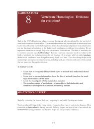
Figure 1 Hypothetical Cooling Curve
FP_dep_DS.wpd 5/29/01
Colligative Properties of Solutions
Experiment 2
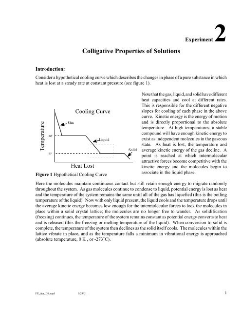
Consider a hypothetical cooling curve which describes the changes in phase of a pure substance in which
heat is lost at a steady rate at constant pressure (see figure 1).
Note that the gas, liquid, and solid have different
heat capacities and cool at different rates.
This is responsible for the different negative
slopes for cooling of each phase in the above
curve. Kinetic energy is the energy of motion
and is directly proportional to the absolute
temperature. At high temperatures, a stable
compound will have enough kinetic energy to
exist as independent molecules in the gaseous
state. As heat is lost, the temperature and
average kinetic energy of the gas decline. A
point is reached at which intermolecular
attractive forces become competitive with the
kinetic energy and the molecules begin to
associate in the liquid phase.
Here the molecules maintain continuous contact but still retain enough energy to migrate randomly
throughout the system. As gas molecules continue to condense to liquid, potential energy is lost as heat
and the temperature of the system remains the same until all of the gas has liquefied (this is the boiling
temperature of the liquid). Now with only liquid present, the liquid cools and the temperature drops until
the average kinetic energy becomes low enough for the intermolecular forces to lock the molecules in
place within a solid crystal lattice; the molecules are no longer free to wander. As solidification
(freezing) continues, the temperature of the system remains constant as potential energy converts to heat
and is released (this the freezing or melting temperature of the liquid). When conversion to solid is
complete, the temperature of the system then declines as the solid itself cools. The molecules within the
lattice vibrate in place, and as the temperature falls a minimum in vibrational energy is approached
(absolute temperature, 0 K , or -273LC).
1

The Freezing Point of Pure Liquid:
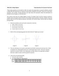
This experiment will focus on the region in which the cooling liquid approaches and achieves the
freezing point (The boxed area on cooling curve in figure 1 is seen close up in figure 2).
Figure 2 Cooling Curve of Liquid Solvent
The Freezing Point of a Solution:
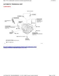
Figure 3 Cooling Curve of Typical Solution
2
At the freezing point both liquid and solid are
present. If the system becomes thermally
insulated from its surroundings, that is, heat
can neither enter or leave the system, a state of
equilibrium will be established. Here the
number of molecules moving from solid to
liquid is the same as the number of molecules
moving from liquid to solid. This means that
the relative quantities of solid and liquid
present will remain constant.
Liquid Solid + Heat
Now consider the effect of a nonvolatile solute upon a freezing solution. Any added solute would
dissolve in the liquid phase and be excluded from the solid crystal lattice. This means that, in effect, the
concentration of liquid solvent molecules has been diminished and the rate of liquid solvent molecules
moving to solid will decrease. On the other hand, the molecules of solid solvent (which remains pure),
continue to move from solid to liquid at the same rate. If the temperature is held at the normal freezing
point of the pure solvent, the system is thrown out of equilibrium and liquid phase is formed at the
expense of solid phase, to a point where only liquid solution is present. In order to reestablish freezing,
the temperature of the system needs to be lowered. This causes heat to be removed from the system and
restores an equilibrium in which solid is present. The solution, therefore, has a lower freezing
temperature than the pure solvent and the freezing point is said to be depressed.
Now as a solution freezes, solvent molecules
are removed from the liquid solution and
deposited on the solid. This increases the
concentration of solute in the liquid solution
and the freezing point further declines. A
solution therefore does not have a sharply
defined freezing point (FP); usually the
freezing point of a solution is taken as the
temperature at which solid solvent crystals
first begin to appear (See figure 3).

The FP depression is one of a set of physical properties of solutions (vapor pressure lowering, boiling
point elevation, and osmotic pressure) known collectively as colligative properties. These properties are
affected by the relative quantity of solute particles to the relative quantity of solvent particles, regardless
of the identity of the solute particles. The FP depression is described quantitatively by the following
equation: FT = k f m. "F" is the number of Celsius degrees the freezing of the solution is depressed
relative to the pure solvent. "m" is the molality of the solution, that is, the number of moles of solute
per one kg of solvent; this relates the quantity of solute to the quantity of solvent. "k f" is the molal
freezing point depression constant and expresses the sensitivity of the solvent to having the its FP
depressed by an added solute. The units are LC/m, which may be viewed as the number of degrees the
FP is depressed per one molal of solute concentration. Each solvent has its own unique value for k f.
E.g., Calculate the FP of a solution containing 600. g of CHCl 3 and 42.0 g of eucalyptol, C 10H 18O,
a fragrant substance found in the leaves of eucalyptus trees. The FP of pure CHCl 3 is -
63.5LC and its k f is 4.68 LC/m.
If a solute is a molecular nonelectrolyte, the solute's molality is a straightforward expression of the
concentration of molecules in solution, that is, the solution's molality. If, however, the solute is a strong
electrolyte, the effective molality is a whole number multiple (called the van't Hoff i factor) of the solute
molality.
Consider a CaCl 2 solution. CaCl 2 is ionic, and each mole of CaCl 2 that dissolves delivers three moles
of ions to the solution, which is indicated by the factor "i":
CaCl 2 (s) ssd Ca +2 (aq) + 2 Cl ( aq) i = 3
The effective molality of the above solution is "im" or 3m and the FP depression equation becomes:
FT = k f i m or FT = k f 3 m
All of the examples in the experimental section to follow will be assumed to remain molecular in
solution and carry an "i" factor of one.
3

Experiment 2
Partner
Name
Colligative Properties of Solutions
EXPERIMENTAL DISCUSSION Experimental Goals:
The experiment to be performed is divided into three sections:
(a) In part A, the FP of the pure solvent, cyclohexane, is determined.
(b) Section B determines the value of the molal freezing point depression constant, k f , of cyclohexane
by measuring the freezing point depression (relative to the FP of pure cyclohexane determined in part
A) of a solution with a known molality of solute.
(c) In part C the molality of cyclohexane solution with an unknown solute is found. This makes possible
the calculation of the molar mass of the unknown.
However, prior to beginning the experiment the temperature probe and CBL must be set up properly.
Setting up the temperature probe and CBL.
1. Plug the temperature probe into the adapter cable. Then plug Probe 1 into Channel 1 of the CBL.
Connect the CBL System to the TI-82 calculator with the link cable using the port on the bottom
edge of each unit. Firmly press in the cable ends.
2. Fill a 1-liter beaker about 4/5 full with ice. Place the 1-liter beaker on the base of the ring stand.
3. Turn on the CBL unit and the TI-82 calculator. Press and select CHEM. Press , then
press again to go to the CHEM MAIN MENU.
4. Set up the calculator and CBL for one temperature probe and one temperature calibration.
Select 1:SET UP PROBES from the CHEM MAIN MENU.
Enter “1” as the number of probes.
Select 1:TEMPERATURE from the SELECT PROBE menu.
Enter “1” as the channel number.
Select 3:USE STORED from the CALIBRATION menu.
5. Set up the calculator and CBL for data collection.
Select 2:COLLECT DATA from the CHEM MAIN MENU.
Select 2:TIME GRAPH from the DATA COLLECTION menu.
Enter “15” as the time between samples, in seconds.
Enter “24” as the number of samples (the CBL will collect data for a total of 6.0 minutes).
Press , then
Select 1:USE TIME SETUP. Do not begin data collection until directed to do so.
5

6
A. FP Determination of Pure Solvent, cyclohexane: In this section, a known mass of solid
cyclohexane will be cooled and its temperature will be measured as it changes with time. This
data will be plotted yielding a graph similar to figure 2. Ideally the plot would show the steady
cooling of the liquid, leading to a constant temperature plateau (the FP or MP) where both the
liquid and solid phases are present (refer again to the boxed area in the cooling curve in figure 1).
The transition from the cooling liquid to the freezing plateau is often marked by irregularities and
temperatures that are temporarily below the actual freezing temperature. This delay is largely
due to the statistical difficulty in achieving the first microscopic seed crystal from the highly
random liquid molecules. Once this tiny cluster forms, individual molecules may easily add to
the crystal, subsequent crystallization is rapid, and the normal freezing temperature is
established.
Laboratory Procedure for Part A:
1) Measure out about 25 mL of dry cyclohexane into one of the clean, dry, large test tube.
2) Carefully push the temperature probe through one of the holes in the two-hole rubber stopper.
Next, carefully insert the metal stirring rod through the remaining hole in the stopper. Fit the
test tube with the two-hole rubber stopper, metal stirring rod, and temperature probe. Carefully
adjust the probe so that the end is at the midpoint of the cyclohexane and centered away from the
walls of the test tube.
3) Clamp the test tube assembly to a ring stand in an upright manner.
4) Check the connections between the probe, the CBL system, and the calculator. Make sure the
CBL and calculator are turned on.
5) Carefully lower the test tube and contents into a 400 mL beaker filled with ice.
6) Cover the ice with a thick layer of NaCl.
7) Stir the cyclohexane gently. Trigger the CBL and stir continuously until the cyclohexane
becomes slushy or until you can no longer move the stirring rod. When collecting temperature
and time data, the TI-82 calculator will automatically shut off after about 5 minutes. This is not
a problem unless the CBL unit finishes collecting data while the calculator is still off (“DONE”
appears on the CBL screen); if this happens, you will lose your data and have to start over. You
can avoid this by watching the calculator screen and promptly turning it back on when you notice
it is blank. So if the TI-82 screen goes blank, quickly press ON to turn the calculator back on.
8) When the CBL unit finishes collecting data raise the test tube assembly out of the ice bath.
9) After the cyclohexane has melted, remove the stopper, stirrer, and temperature probe assembly
from the test tube and set aside to dry. Cover the large test tube containing the cyclohexane and
save for later use.

Data Workup for Part A:
1. Press to display a graph of temperature vs. time. Use to examine the data points
along the curve. As you move the cursor right or left, the time (X) and temperature (Y) values
of each data point are displayed below the graph. Based on your data, what was the freezing
temperature of pure cyclohexane (to the nearest 0.1LC)? Show this to your instructor.
2) Copy the data in L2 from the calculator memory into the data table below.
3) For the lab write-up you will need to prepare a cooling curve by plotting temperature along the
y-axis versus time in seconds along the x-axis using a spread sheet. Turn off the line in the
spreadsheet so the graph shows only the data point themselves. In order to maximize precision,
expand the scale along each axis as much as possible so the data plots allow the reading of the
temperature on the graph to ±0.1 LC. Along both the cooling-liquid portion of the data and along
the freezing portion, draw for each the best straight line possible (use a straight edge) that gives
a weighted average of all the data points (see figure 2). Note that no one data point is required
to fall on this line; in fact, it is possible that none of these points may fall on this line. The
intersection of these two lines in the region of supercooling yields the best estimate of the
freezing temperature of the liquid. Record this temperature on the data sheet below (with
greatest possible precision) as the observed freezing point of pure cyclohexane.
Data Table for Part A:
15 s________ 105 s________ 195 s________ 285 s________
30 s________ 120 s________ 210 s________ 300 s________
45 s________ 135 s________ 225 s________ 315 s________
60 s________ 150 s________ 240 s________ 330 s________
75 s________ 165 s________ 255 s________ 345 s________
90 s________ 180 s________ 270 s________ 360 s________
Observed FP of pure cyclohexane:_________
7

8
B. Determination of k f of cyclohexane: In this procedure, the molal freezing point depression
constant, k f , of cyclohexane will be determined experimentally. The freezing temperature will
be found for a solution using a known mass of cyclohexane as the solvent and a measured mass
of naphthalene as the solute. The freezing point depression, FT , of the solution is found by
calculating the difference between the freezing temperature of the solution and the freezing
temperature of the pure solvent found in part A. After the molality of the solution, m , is
computed from the known masses of solute and solvent, the k f may be calculated: k f = FT/ m
Laboratory Procedure for Part B:
1) Place the second large, dry test tube into a 250 mL erlenmeyer flask with the tube up-right.
Weigh and record on the data sheet below the combined mass of this setup to the nearest 0.001 g
on the electronic reagent balance in the laboratory. Carefully, add about 1.0 g of naphthalene to
the test tube, and record the mass of the naphthalene and glassware to the nearest 0.001 g.
2) Carefully pour the cyclohexane from the first test tube into the second tube. Weigh and record
the mass of the flask, test tube and contents to the nearest 0.001 g. Set the empty first test tube
aside to dry for later use in Part C.
3) Fit the second test tube with the stopper, stirring rod, and temperature probe. Carefully adjust
the probe so that the end is at the midpoint of the cyclohexane and centered away from the walls
of the test tube.
4) Attach the probe to the CBL system as before.
5) Re-set the CBL to take data every 15 seconds in “time graph” mode.
6) Carefully lower the test tube and contents into the beaker filled with the ice and NaCl mixture.
7) Stir the cyclohexane gently. Trigger the CBL and stir continuously until the cyclohexane
becomes slushy or until you can no longer move the stirring rod.
8) When the CBL unit finishes collecting data raise the test tube assembly out of the ice bath.
9) After the cyclohexane has melted, remove the stopper, stirrer, and temperature probe assembly.
Discard the cyclohexane/naphthalene mixture into the proper waste container. Rinse the stopper
assembly with fresh cyclohexane being sure to collect the rinse and to discard it into the waste
container. Set the assembly aside to dry for use in Part C.

Data Workup for Part B:
1. Press to display a graph of temperature vs. time. Use to examine the data points
along the curve. As you move the cursor right or left, the time (X) and temperature (Y) values
of each data point are displayed below the graph. Based on your data, what was the freezing
temperature of cyclohexane/naphthalene mixture (to the nearest 0.1LC)?
Show this to your instructor.
2) Copy the data in L2 from the calculator memory into the data table below.
3) As in Part A, prepare a cooling curve by plotting temperature along the y-axis versus time in
seconds along the x-axis using a spread sheet. Turn off the line in the spreadsheet so the graph
shows only the data point themselves. Use a straight edge to draw a line through the data along
both the cooling-liquid portion of the data and along the freezing portion. Remember that as the
solution freezes, the liquid becomes ever more concentrated in solute, and the freezing
temperature steadily decreases. The intersection of these two lines in the region of supercooling
yields the best estimate of the freezing temperature of the mixture. Record this temperature on
the data sheet (with greatest possible precision) as the observed freezing point of the solution.
Data Table for Part B:
Mass of test-tube and flask:____________
Mass of test-tube, flask, and naphthalene:____________
Calculated mass of naphthalene:____________
Mass of test-tube, flask, naphthalene and cyclohexane:____________
Temperature/time data:
Calculated mass of cyclohexane:____________
15 s________ 105 s________ 195 s________ 285 s________
30 s________ 120 s________ 210 s________ 300 s________
45 s________ 135 s________ 225 s________ 315 s________
60 s________ 150 s________ 240 s________ 330 s________
75 s________ 165 s________ 255 s________ 345 s________
90 s________ 180 s________ 270 s________ 360 s________
Observed FP of cyclohexane/naphthalene solution: ___________
9

10
C. Determination of the Molar Mass of the Unknown: In this section, a measured mass of an
unknown solute will be added to a fresh sample of cyclohexane solvent, whose mass is also
known. The freezing point depression, FT, of this solution will be determined. Since k f has
been found in part B, the molality of the solution containing the unknown, m, may be calculated:
m = FT/k f. The molality, which is in units of moles solute per kg of solvent, may now be used
to find the number of moles of unknown solute present, and, since the mass of the unknown was
determined in the beginning, the molar mass may now be calculated. Watch your units. They
insure a proper sequence of calculations.
Laboratory Procedure for Part C:
1) Obtain your unknown. Record this number on the data sheet.
2) Place the remaining dry, large test tube into a 250 mL erlenmeyer flask with the tube up-right.
Weigh and record the combined mass of this setup to the nearest 0.001 g.
3) Carefully pour your entire unknown into the test tube and re-weigh the entire apparatus to the
nearest 0.001g.
4) Measure out about 25 mL of fresh cyclohexane with a graduated cylinder and pour it carefully
into the test tube with your unknown being sure to rinse down the inside wall of the tube with
the cyclohexane.
5) Fit the test tube with the stopper, stirring rod, and temperature probe. Carefully adjust the probe
so that the end is at the midpoint of the cyclohexane and centered away from the walls of the test
tube.
6) Attach the probe to the CBL system as before. Re-set the CBL to take data every 15 seconds in
“time graph” mode.
7) Carefully lower the test tube and contents into the beaker filled with ice/salt mixture.
8) Stir the cyclohexane gently. Trigger the CBL and stir continuously until the cyclohexane
becomes slushy or until you can no longer move the stirring rod.
9) When the CBL unit finishes collecting data raise the test tube assembly out of the ice bath.
10) After the cyclohexane has melted, remove the stopper, stirrer, and temperature probe assembly.
Discard the cyclohexane/unknown mixture into the proper waste container. Rinse the stopper
assembly with fresh cyclohexane being sure to collect the rinse and to discard it into the waste
container. Return the equipment.

Data Workup for Part C:
1. Press to display a graph of temperature vs. time. Use to examine the data points
along the curve. As you move the cursor right or left, the time (X) and temperature (Y) values of
each data point are displayed below the graph. Based on your data, what was the freezing
temperature of cyclohexane/unknown mixture (to the nearest 0.1LC)?
Show this to your instructor.
2) Copy the data in L2 from the calculator memory onto your lab.
3) As in Part A, prepare a cooling curve by plotting temperature along the y-axis versus time in
seconds along the x-axis using a spread sheet. Turn off the line in the spreadsheet so the graph
shows only the data point themselves. Use a straight edge to draw a line through the data along
both the cooling-liquid portion of the data and along the freezing portion. Remember that as the
solution freezes, the liquid becomes ever more concentrated in solute, and the freezing
temperature steadily decreases. The intersection of these two lines in the region of supercooling
yields the best estimate of the freezing temperature of the mixture. Record this temperature on
the data sheet (with greatest possible precision) as the observed freezing point of the
cyclohexane/unknown solution.
Data Table for Part C:
Mass of test-tube and flask:____________
Mass of test-tube, flask, and unknown:____________
Calculated mass of unknown:____________
Mass of test-tube, flask, unknown and cyclohexane:____________
Temperature/time data:
Calculated mass of cyclohexane:____________
15 s________ 105 s________ 195 s________ 285 s________
30 s________ 120 s________ 210 s________ 300 s________
45 s________ 135 s________ 225 s________ 315 s________
60 s________ 150 s________ 240 s________ 330 s________
75 s________ 165 s________ 255 s________ 345 s________
90 s________ 180 s________ 270 s________ 360 s________
Observed FP of cyclohexane/unknown solution: ___________
11

12
CALCULATIONS/QUESTIONS
1. a) From the freezing points of pure cyclohexane and the cyclohexane/naphthalene solution,
calculate the freezing point depression, FT , of the cyclohexane/naphthalene solution.
b) For the cyclohexane/naphthalene solution in part B, calculate the number of moles of
naphthalene added (naphthalene, C 10H 8). Then calculate the molality of the solution.
c) From the molality of the cyclohexane/naphthalene solution just calculated, and the freezing
point depression, FT , of the cyclohexane/naphthalene solution, calculate the value of the molal
freezing point depression constant, k f , for cyclohexane.
2. a) From the freezing points of pure cyclohexane and the cyclohexane/unknown solution, calculate
the freezing point depression, FT , of the cyclohexane/unknown solution.
b) From the k f of cyclohexane calculated above and the freezing point depression, FT , of the
cyclohexane/unknown solution in 2a, calculate the molality, m , of the cyclohexane/unknown
solution.
c) For part C, having measured the mass of the unknown acid solute and the mass of the
cyclohexane solvent, and having just found the molality of the cyclohexane/unknown solution,
calculate the apparent molar mass of the unknown.