- Page 1 and 2:
October 2012 Volume 15 Number 4
- Page 3 and 4:
Supporting Organizations Centre for
- Page 5 and 6:
Peer Evaluation in Blended Team Pro
- Page 7 and 8:
The contribution entitled “Semant
- Page 9 and 10:
with the group exploration activity
- Page 11 and 12:
Data collection This study collecte
- Page 13 and 14:
Table 2. The mind mapping activitie
- Page 15 and 16:
On the contrary, the students in th
- Page 17 and 18:
Elwart-Keys M., Halonen D., Horton
- Page 19 and 20:
Zualkernan, I. A., Raza, A., & Kari
- Page 21 and 22:
In summary, a large base of school
- Page 23 and 24:
Usability deals with how easy it is
- Page 25 and 26:
As Figure 5 shows, the adoption mod
- Page 27 and 28:
Adoption Factors of Adoption An ari
- Page 29 and 30:
that the particular way of using th
- Page 31 and 32:
Stoyanova, E. (2005). Problem posin
- Page 33 and 34:
The impact of peer assessment has b
- Page 35 and 36:
e used for the setup of diagnostic
- Page 37 and 38:
RQ2: Does assessing solutions of ot
- Page 39 and 40:
Both components, authoring tool and
- Page 41 and 42:
Supervision We enhanced the player
- Page 43 and 44:
Stepanyan, K., Mather, R., Jones, H
- Page 45 and 46:
international group of experts and
- Page 47 and 48:
1. Web application development over
- Page 49 and 50:
In Mike’s terminal window, run
- Page 51 and 52:
Chen, L.-C., & Lin, C. (2007). Comb
- Page 53 and 54:
To address these drawbacks some app
- Page 55 and 56:
LOM LOM objects Universia RDF repos
- Page 57 and 58:
Obtain DBpedia categories. In this
- Page 59 and 60:
This is not the usual result since
- Page 61 and 62:
The algorithm returns a set of DBpe
- Page 63 and 64:
shows. However, the benefit of expl
- Page 65 and 66:
Conclusions An approach for the ext
- Page 67 and 68:
Zhao, G., Ailiya, & Shen, Z. (2012)
- Page 69 and 70:
Apart from these, a project “SimS
- Page 71 and 72:
Autonomy is related to the sense of
- Page 73 and 74:
practice” for practicability, and
- Page 75 and 76:
secondary school students in Singap
- Page 77 and 78:
desirable; the event endurer is the
- Page 79 and 80:
Gartner, A. (1971). Children Teach
- Page 81 and 82:
experience and the guidance which i
- Page 83 and 84:
is further augmented with the numbe
- Page 85 and 86:
shown in the central part of Figure
- Page 87 and 88:
useful when choosing a learning pat
- Page 89 and 90:
competences helped them to specific
- Page 91 and 92:
model (Maier & Schmidt, 2007) as an
- Page 93 and 94:
Margaryan, A., Milligan, C., Little
- Page 95 and 96:
Being a Digital Native, however, is
- Page 97 and 98:
Pre-adolescent information seeking
- Page 99 and 100:
The significance of the study rests
- Page 101 and 102:
The middle school site followed a s
- Page 103 and 104:
A similar process for the middle sc
- Page 105 and 106:
have developed a new design model
- Page 107 and 108:
Davidson, J., & Wright, J. (1994).
- Page 109 and 110:
Mostmans, L., Vleugels, C., & Banni
- Page 111 and 112:
productive and needing more time to
- Page 113 and 114:
the location of computers: In eleme
- Page 115 and 116:
Accordingly, informants in the BOM-
- Page 117 and 118:
Goodman, L., MacCallum-Stewart, E.d
- Page 119 and 120:
Chen, M.-Y., Chang, F. M.-T., Chen,
- Page 121 and 122:
information systems (system quality
- Page 123 and 124:
participant’s usage intentions we
- Page 125 and 126:
service quality of IS functions. We
- Page 127 and 128:
the e-Portfolio system. Therefore,
- Page 129 and 130:
other colleges/universities to avoi
- Page 131 and 132:
Cho, C.-W., Yeh, T.-K., Cheng, S.-W
- Page 133 and 134:
them search for resources, they wer
- Page 135 and 136:
A user’s tags can be visible or i
- Page 137 and 138:
a month. Note that, since social ta
- Page 139 and 140:
(Fujimura et al., 2007). The aim of
- Page 141 and 142:
Rainie, L. (2007, January 31). 28%
- Page 143 and 144:
Moreover, teacher pedagogical belie
- Page 145 and 146:
However, Singer and Maher (2007) ex
- Page 147 and 148:
Data analysis After collecting data
- Page 149 and 150: interpretations of effect size of c
- Page 151 and 152: places to develop teaching skills,
- Page 153 and 154: Kajder, S. B. (2005). Preservice En
- Page 155 and 156: Huang, Y.-M., Liu, C.-H., Lee, C.-Y
- Page 157 and 158: organized in a didactic way that co
- Page 159 and 160: Front-end subsystem A front-end sub
- Page 161 and 162: possible location of the visitor, t
- Page 163 and 164: Procedure Figure 7. The participant
- Page 165 and 166: Results of user satisfaction evalua
- Page 167 and 168: Table 8. The comparison of the PSQ
- Page 169 and 170: system for recommendation purpose i
- Page 171 and 172: affiliation network models as a col
- Page 173 and 174: Choosing the most suitable viewer i
- Page 175 and 176: visualization, user-friendly operat
- Page 177 and 178: Figure 3. Example of cutting tool w
- Page 179 and 180: imported in Adobe Acrobat Pro Exten
- Page 181 and 182: 10 points, if it fully meets the re
- Page 183 and 184: The overall competitive assessment
- Page 185 and 186: Ramos Barbero, B., García Maté, E
- Page 187 and 188: connected devices such as iPods and
- Page 189 and 190: The common constructivist themes su
- Page 191 and 192: Data analysis Data was gathered fro
- Page 193 and 194: ...I do my downloads through iTunes
- Page 195 and 196: podcasts. In Case Study 2, although
- Page 197 and 198: Rüdel, C. (2006). A work in progre
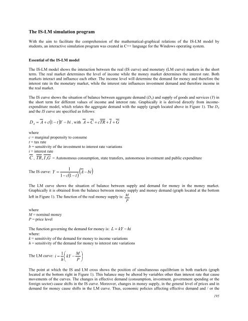
- Page 199: issues in undergraduate economics c
- Page 203 and 204: Through the simulation program the
- Page 205 and 206: However, group A presents a better
- Page 207 and 208: Thus, we can confirm the advantages
- Page 209 and 210: Clark, D., Nelson, B., Sengupta, P.
- Page 211 and 212: centered approach to learning inste
- Page 213 and 214: Research question and population Th
- Page 215 and 216: Learning effectiveness was analyzed
- Page 217 and 218: that have turned experimental equip
- Page 219 and 220: Lee, H.-J., & Lim, C. (2012). Peer
- Page 221 and 222: Message Analysis Frameworks Existin
- Page 223 and 224: social messages, whereas the latter
- Page 225 and 226: This finding has significant implic
- Page 227 and 228: These results imply that students e
- Page 229 and 230: Lee, H.-J. & Kim, I. (2011). Develo
- Page 231 and 232: We have successfully experimented o
- Page 233 and 234: Figure 1. Analysis of the XO-1, the
- Page 235 and 236: Figure 4. The most popular coping s
- Page 237 and 238: other way too, when children were a
- Page 239 and 240: judge or ridicule them. It is impor
- Page 241 and 242: Acknowledgements This research rece
- Page 243 and 244: Tambouris, E., Panopoulou, E., Tara
- Page 245 and 246: participatory or collaborative prac
- Page 247 and 248: My Desk is a workspace personal to
- Page 249 and 250: While the notion of grouping learne
- Page 251 and 252:
Teacher controlled Teacher controll
- Page 253 and 254:
opinion of collaboration facilities
- Page 255 and 256:
Acknowledgements Work presented in
- Page 257 and 258:
Tsai, P.-S., Hwang, G.-J., Tsai, C.
- Page 259 and 260:
owsing, title browsing and author b
- Page 261 and 262:
The simple search function Figure 4
- Page 263 and 264:
The author browse function Figure 8
- Page 265 and 266:
Comparisons of usage feedback betwe
- Page 267 and 268:
Conclusions In the past decades, va
- Page 269 and 270:
Appendix A: The final version of qu
- Page 271 and 272:
as validity should be investigated.
- Page 273 and 274:
of the assessment results across th
- Page 275 and 276:
Figure 1. Teachers were allowed to
- Page 277 and 278:
Table 3 summarized the Pearson’s
- Page 279 and 280:
achievement test scores. Given thes
- Page 281 and 282:
Russell, J. D., & Butcher, C. (1999
- Page 283 and 284:
Attitude 4-5. Reflection on peer pe
- Page 285 and 286:
universities participate in new mar
- Page 287 and 288:
Agreement on a joint diploma/degree
- Page 289 and 290:
1. Awareness of the benefits for st
- Page 291 and 292:
Institutional resistance to change
- Page 293 and 294:
Business model A business model can
- Page 295 and 296:
The identity provider is responsibl
- Page 297 and 298:
Sample scenario Business layer The
- Page 299 and 300:
executed to fulfil collaboration ag
- Page 301 and 302:
Cadima, R., Ojeda, J., & Monguet, J
- Page 303 and 304:
Centrality metrics measure the exte
- Page 305 and 306:
Results Social Networks During the
- Page 307 and 308:
performance of the executives educa
- Page 309 and 310:
Song, S., Nerur, S., & Teng, J. (20
- Page 311 and 312:
We also propose a specific implemen
- Page 313 and 314:
assessment outputs gathering during
- Page 315 and 316:
is an authoring platform created wi
- Page 317 and 318:
Figure 4. Example of an assessment
- Page 319 and 320:
ate of errors in “Level 3” foll
- Page 321 and 322:
The evaluation of reusing pedagogic
- Page 323 and 324:
Shute, V. J., & Spector, J. M. (200
- Page 325 and 326:
Literature Review Cognitive apprent
- Page 327 and 328:
questions. Meta-Analyzer has been r
- Page 329 and 330:
presentation as a conclusion. Simil
- Page 331 and 332:
Interaction effect between cognitiv
- Page 333 and 334:
References Abouserie, R., & Moss, D
- Page 335 and 336:
Oloruntegbe, K. O., Ikpe, A., & Kuk
- Page 337 and 338:
Young, M.-L. (2012). An Exploratory
- Page 339 and 340:
use is simply an expedited form of
- Page 341 and 342:
In order to elicit narratives about
- Page 343 and 344:
Findings The study shows that deliv
- Page 345 and 346:
With the changes in the teaching en
- Page 347 and 348:
Bostrom, R. & Heinen, J. S. (1977a)
- Page 349 and 350:
Lindgren, R., & McDaniel, R. (2012)
- Page 351 and 352:
those that allow for less agentic a
- Page 353 and 354:
whether the adoption of a novel des
- Page 355 and 356:
AEM Course Features. A subset of po
- Page 357 and 358:
Figure 4 shows the average pre and
- Page 359 and 360:
Ford, M. (1992). Motivating humans:
- Page 361 and 362:
Liang, T.-H., Huang, Y.-M., & Tsai,
- Page 363 and 364:
TSL1: Teacher as a coach TSL2: Teac
- Page 365 and 366:
instructional event (the upper part
- Page 367 and 368:
Table 3. The results of the chi-squ
- Page 369 and 370:
simultaneously complied with ISL an
- Page 371 and 372:
Finally, several pedagogical implic
- Page 373 and 374:
Hung, C.-M., Hwang, G.-J., & Huang,
- Page 375 and 376:
theory of Piaget (1950) and the soc
- Page 377 and 378:
Learning activities The unit of “
- Page 379 and 380:
subgroup in the control group neede
- Page 381 and 382:
When asked about the differences be
- Page 383 and 384:
Delialioglu, O., Cakir, H., Bichelm
- Page 385 and 386:
Anderson, T., & McGreal, R. (2012).
- Page 387 and 388:
This belief in the correlation of r
- Page 389 and 390:
and sometimes to compel, faculty to
- Page 391 and 392:
Part time versus full time faculty
- Page 393 and 394:
The open universities have a partic