IMPLEMENTATION OF MATRIX CONVERTER CONTROL CIRCUIT ...

IMPLEMENTATION OF MATRIX CONVERTER CONTROL
CIRCUIT WITH DIRECT SPACE VECTOR MODULATION AND
FOUR STEP COMMUTATION STRATEGY
Tadra Grzegorz, University of Zielona Gora, Poland
Abstract
In this paper a matrix converter control circuit
with implemented vector modulation and four-step
commutation strategy is described. The presented
control circuit consists of two DSP processors and
FPGA. The matrix converter is a device build with 9
bidirectional switches (18 IGBT transistors). The
Control circuit in contest makes possible of the
matrix converter output voltage amplitude and
frequency change, in addition input power factor can
be controlled. Some simulation and experimental
tests results of the ca. 1 kVA matrix converter
laboratory model controlled by described control
circuit are shown.
1. Introduction
In recent years transformation and control of
energy has been mostly realized with indirect AC-AC
converters with DC link. An alternative for this
solution is still searched for. One of the recently
considered alternatives is Matrix Converter (MC).
The MC is a direct energy converter (build with nine
bidirectional switches) able to connect every output
phase to every input phase and on this principle
deliver output power with desired frequency.
The main advantages of the MC are: 1- lack of
the DC link energy storage device, 2- generation of
the load voltages with arbitrary amplitude and
frequency, 3- sinusoidal input and output currents, 4-
possibility to control input power factor, 5-
regeneration capability. The basic disadvantages are:
1- maximum input/output voltage transfer ratio by
sinusoidal current shape below 1 by most control
strategies, 2- sensitivity to the disturbance of the
input voltage systems.
There are two main concepts of MC control
strategies: the first based on low frequency transfer
matrix (for example: scalar [20] control strategy or
control strategy proposed by Venturini [1], [2]) and
the second based on currents and voltages space
vector (SV) representations (for example direct [5]-
[11] or indirect [3] space vector control strategy).
A direct space vector modulation (SVM) does not
need fictitious DC link or addition of the third-
harmonic as in other common MC control strategies.
XI International PhD Workshop
OWD 2009, 17–20 October 2009
321
Maximal voltage transfer ratio for this strategy is
0,866. Furthermore control of the input power
factor is realized regardless of the output power
factor [5]-[10]. Because of those advantages the
strategy (after some modifications) will be
implemented in Matrix Reactance Frequency
Converters (MRFC). The converters have been
studied by Professor Fedyczak’s team at the
University of Zielona Góra. Implementation of the
SVM for MRFC is going to be a part of the author’s
PhD work. MRFC is based on a unipolar PWM AC
matrix reactance choppers (MRC), description of the
MRFC family (9 topologies) is included in [15] and
[16]. In MRFC both a frequency change and the
buck-boost load voltage conversion are possible
[12]-[19].
This paper presents project as well as simulation
and experimental tests results of the MC control
circuit with implemented direct (SVM) and four-step
current commutation control strategy. Presented
control circuit is going to be a part of the MRFC
with modified direct SVM.
Next section contains description of the matrix
converter and it’s control circuit. Basing on [5]-[8]
and [11] implemented control and commutation
strategy is described in section 3. In section 4 some
simulation and experimental test results are shown.
Conclusion follows in the last section.
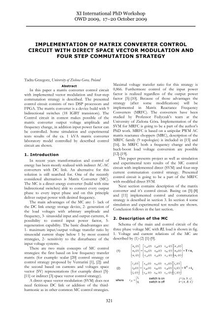
2. Description of the MC
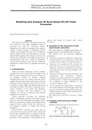
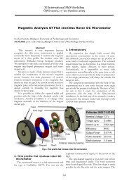
Schema of the main and control circuit of the
three phase voltage MC with RL load is shown in fig.
1. Voltage and current relations of the MC are
described by (1)-(2) [1]-[9].
⎡ua
( t)
⎤ ⎡saA
( t)
saB
( t)
saC
( t)
⎤⎡u
A ( t)
⎤
⎢ ⎥ ⎢
⎥⎢
⎥
(1) ⎢
ub
( t)
⎥
=
⎢
sbA
( t)
sbB
( t)
sbC
( t)
⎥⎢
u B ( t)
⎥
= T × ui
⎢⎣
uc
( t)
⎥⎦
⎢⎣
scA
( t)
scB
( t)
scC
( t)
⎥⎦
⎢⎣
uC
( t)
⎥⎦
⎡iA
( t)
⎤ ⎡s
aA ( t)
sbA
( t)
scA
( t)
⎤⎡ia
( t)
⎤
⎢ ⎥ ⎢
⎥⎢
⎥ T
(2) ⎢
iB
( t)
⎥
=
⎢
saB
( t)
sbB
( t)
scB
( t)
⎥⎢
ib
( t)
⎥
= T × i o
⎢⎣
iC
( t)
⎥⎦
⎢⎣
saC
( t)
sbC
( t)
scC
( t)
⎥⎦
⎢⎣
ic
( t)
⎥⎦
where
s jk
⎧1,
= ⎨
⎩0,
switch is on
switch is off
j={a, b, c},
k={A, B, C}

Fig. 1. Three- phase Matrix Converter
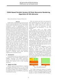
MC can theoretically assume 512 (2 9) switching
configurations (SC) but because of commutation
lows there are only 27 SC permitted among which 21
SC (18 active and 3 zero), are engaged in direct SVM
[3]-[8]. Geometrical interpretations of those 21 SC
are shown in fig. 3.
Fig. 2. Geometrical interpretation of the 21 switch
configurations engaged in direct SVM.
Using transformation (3) input and output voltages
and currents of the MC can be represented as space
vectors.
(3)
2 j(
2π
/ 3)
j(
4π
/ 3)
x = ( x1
+ x2e
+ x3e
3
Where x 1
, x 2
, x 3
– instantaneous values of the transformed
signals.
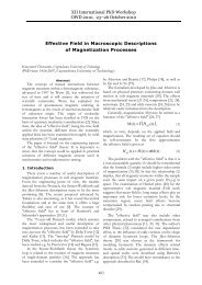
The geometrical interpretations of the space-
vector representations of the line to neutral load
voltages (uaN, ubN, ucN) and input line currents (iA, iB,
iC), created for all active and zero SC (fig. 2)
according to (3) are shown in fig.3. Furthermore
numbers of the sectors (Si, So) between those
vectors are introduced [7].
Because of MC complexity its control and
commutation strategy is complicated and demands
advanced hardware solutions. That is why presented
control circuit consists of two DSP processors
(ADSP 21368), three A/D converters and a FPGA
circuit (fig. 1). Basic specifications data for those
components are collected in table 1. Using this
control circuit instantaneous space- vector
representations of the source currents are calculated.
)
322
Based on those calculations proper switching
sequence can be found to form desired load voltage
vector. This process will be described in detail in the
next section.
Fig. 3. Space vector representations for, a) load line to
neutral voltages (uaN, ubN, ucN), b) input line currents
jα
0 u 0 = e
- exemplary line to neutral load voltages
jβ
i i
vector position, i = e
- exemplary line source currents
vector position,, So- sector No. for u0, Si- sector No. for ii
Table. 1 Specifications data for control circuit
components
Component Specification
Processor DSP
(ADSP-21368)
ALS-3G-2368
PCI
FPGA (XS3S200)
Converters
A/D – D/A
ALS-3G-
ACA1812-1
Manufactured by Analog Devices;
clock speed 400 MHz; 1600 MFLOPS;
2 Mbit SRAM; 6 Mbit ROM
Manufactured by Xilnix; clock speed
10 MHz; programable system gates:
200000, 216kbajtów RAM
18 bit A/D converter; convertion speed
up to 570 kSps, input voltage range: +/-
2,48V
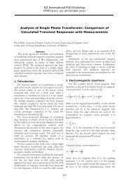
3. Control and commutation strategy
Functional schema of the implemented control
and commutation strategy and tasks division for
control circuit components are shown in fig. 4.
Because of MC source currents distortion their space
vector representation ii is determined basing on
measured source phase voltages. The way in with

source currents vector position is define, based upon
source voltages vector position (calculated according
to (3)) is shown in fig. 6b. Load voltages space
vector uo, with desired amplitude and angular
velocity ωout, is also calculated according to (3). In
the next step according to fig. 3 previously calculated
ii and uo positions allows sector numbers S0, Si and
phase angels α’0, β’i to be identified. It has to be
mentioned that phase angels α’0, β’i are defined with
respect to bisecting line of suitable sector, limited
according to (4) and differ then α0, βi (fig. 3, fig. 6)
[7].
(4) − π 6 < α'0
< π 6 π 6 < β ' < π 6
ALS-3G-2368 PCI
21 SC.
(fig. 2)
saA
ia ib ic
β’i
IDENTIFICATION
(4)
ON-TIME
RATIOS
CALCULATION
(5)-(8)
VECTOR
SELECTION
(tab. 1, tab. 2)
saB saC
SIGNAL CHANGE
DETECTION
SWITCH SEQUENCE
SELECTION
Tseq
TRANSISTOR
CONTROL SIGNALS
So IDENTIFICATION (rys. 3b)
α’0
IDENTIFICATION
(4)
Si IDENTIFICATION (Rys. 3a)
SWITCH- ON TIMES
CALCULATION (9),(10)
(rys. 9)
sbA sbB sbC
SWITCH SEQUENCE
SELECTION
− i
uB
uC
CALCULATION OF THE SOURCE CURRENTS
VECTOR REPRESENTATION (3)
SWITCHING PATTERN
(11), (12), (fig. 6)
CONTROL SIGNALS FOR BIDIRECTIONAL
SWITCHES
SIGNAL CHANGE
DETECTION
(rys. 9)
TRANSISTOR
CONTROL SIGNALS
scA scB scC
(rys. 9)
SIGNAL CHANGE
DETECTION
SWITCH SEQUENCE
SELECTION
TRANSISTOR
CONTROL SIGNALS
TaA1 TaA2 TaB1 TaB2 TaC1 TaC2 TbA1TbA2 TbB1 TbB2 TcC1 TcC2 TbA1TbA2 TbB1 TbB2 TcC1 TcC2
A
uA
D
A
D
A
D
LOAD VOLTAGE
VECTOR
DETERMINATION (3)
φi
q
ωout
Fig. 4. General description of the implemented control
and commutation strategy.
φ i - input current displacement angle, ω out - output voltage
pulsation, q - voltage transfer ratio, T seq -switching time
period.
Subsequently four on-time ratios according to
(5)-(7) are calculated. Furthermore during every
sequence period, based on knowledge about actual
sectors and signs of the on-time ratios, according to
table 2 and 3 four active and one zero SC are
selected. Switched-on times for selected SC are
calculated from (5)-(7) and expressed by (9), (10).
(5)
(6)
(7)
S Si
1 2 cos( α'
π 3)
cos( β '
q
i
π 3)
δ ( 1)
0 + +
0
−
−
1
= −
3
cosϕ
i
δ = ( −1)
2
δ = ( −1)
3
S0
+ Si
S0+
Si
2 cos( α'0
−π
3)
cos( β'
i + π 3)
q
3
cosϕ
2 cos( α'0
+ π 3)
cos( β'i
−π
3)
q
3
cosϕ
i
i
323
(8)
δ = ( −1)
4
(9) t1 = 1 Tseq
(10)
S0
+ Si
+ 1
2 cos( α '0
+ π 3)
cos( β 'i
+ π 3)
q
3
cosϕ
δ ;
t2 = δ 2 Tseq
;
t3 = δ3
Tseq
;
t4 = δ 4
t = δ T = T − δ + δ + δ + δ ) T
0
0
seq
seq
( 1 2 3 4
i
Tseq
Table 2. Summary of the active configurations assigned
to sectors and on-time ratios.
(Si = 1or4)&(So=1or4) 19 16 21 18 7 4 9 6
(Si = 2or5)&(So=1or4) 17 20 19 16 5 8 7 4
(Si = 3or6)&(So=1or4) 21 18 17 20 9 6 5 8
(Si = 1or4)&(So=2or5) 13 10 15 12 19 16 21 18
(Si = 2or5)&(So=2or5) 11 14 13 10 17 20 19 16
(Si = 3or6)&(So=2or5) 15 12 11 14 21 18 17 20
(Si = 1or4)&(So=3or6) 7 4 9 6 13 10 15 12
(Si = 2or5)&(So=3or6) 5 8 7 4 11 14 13 10
(Si = 3or6)&(So=3or6) 9 6 5 8 15 12 11 14
δ1>0 δ10 δ20 δ30 δ40 -δ4 δ4 -δ4 δ4 -δ4
Selected switching configurations (vectors) are
turned on according to the sequence described by
(11), where for example ½δ3 means that SC selected
according to above described principles and assigned
in table 2 to δ3 must be switched on as the first one
for the time ½t3. This switching pattern was achieved
by comparison of the modulation waves with saw
wave as it is shown in fig. 5. As a result of this
comparison during every switching period Tseq local
duty cycles d0-d4 for individual transistors are
worked out.
(11)
(12)
x
d1
1 1 1 1
δ3
→ δ1
→ δ 2 → δ 4 → δ0
2 2 2 2
1 1 1 1
→ δ 4 → δ 2 → δ1
→ δ3
2 2 2 2
= δ ; x
3
x
d
d
2
4
= δ + δ ; x
3
1
= δ + δ + δ + δ ;
3
1
d
2
3
seq
= δ + δ + δ ;
0 0.5 1 1.5 2
Fig. 5. Switching pattern description
In fig. 6 there is an example how vector uo, which
represents instantaneous values of the load phase
voltages, and vector ii, which represents
instantaneous values of the source currents is
formed. .Vector u0 is set up of two components u’0
and u’’0 , which are created by switching on earlier
selected vectors (in ex. 7, 16, 21, 6, 1) through
suitable times (9), (10) during the cycle period.
Furthermore in Fig. 4b) it is shown how the control
4
3
1
2

of φi (input power factor) is achieved by controlling
βi. It has to be accounted that:
(13) q = 0,
866 ⋅cos(
ϕ )
max i
Fig. 6 Vector modulation principle a) for exemplary
output voltage vector position, b) for exemplary input
current vector position.
In fig. 7a a fragment of MC from fig .1 is shown.
Bidirectional switch S cB (T cB1 ,T cB2) cannot be
switched on in the same time when S cC (T cC1 ,T cC2) is
switched off because of the finite turn-on and turnoff
times. In such switch state short-circuit or
overvoltage can occur which can cause
semiconductor damage. To avoid such switch states
in presented control circuit a four step current
commutation strategy is implemented. In fig. 7b an
exemplary commutation diagram between SBc and
SCb is shown. In fig. 8a transition diagram which
presents how this commutation strategy is realized in
FPGA (fig. 1, fig. 4) is shown.
Fig. 7 Commutation in MC, a) fragment of MC- two
bidirectional switches b) commutation diagram for SBc
and SCb. td – duration of commutation steps.
Rys. 8. Transition diagram of the implemented in FPGA
four step current commutation strategy
Where: OUT={Tak1, Tak2, Tbk1, Tbk2, Tck1, Tck2}- actual transistors
states, Current_SC={Tak1, Tak2, Tbk1, Tbk2, Tck1, Tck2} transistors
states before commutation request , New_SC={Tak1, Tak2, Tbk1,
Tbk2, Tck1, Tck2}- final transistor states, Tx- transitions, Sx-
steps
324
4. Simulation and experimental test
results
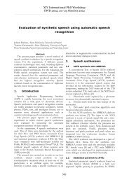
A photograph of the MC prototype for which the
described control circuit was designed is shown in
fig. 9. the MRFC are also researched with this
prototype[19]. Simulation tests ware obtained by
Matlab Simulink. Simulation and experiment
parameters are collected in table 4.
Table 4. Simulation and experiment parameters.
Parameter Symbol Value
Source
Simulation Experiment
amplitude and
frequency
Us / f 230 V/50
Hz
62 V / 50 Hz
Switching
time period
Tsequ 2 ms
Inductivities
LF LL 1,5 mH
10 mH
Capacitors CF 10 µF
Resistance RL 60 Ω
Rys. 9. Matrix converter prototype
1 – input filter; 2 – AC adapter; 3 – FPGA board
(ZL9PLD); 4 – optical transmitters; 5 – load current
measurement circuit; 6- source voltage measurement
circuit; 7 – optical receivers and transistor drivers; 8 –
protection lamp circuit; 9 – load induction; 10 – load
resistance; 11 –DSP board (ALS-G3-2368PCI) 12 – A/D
converters (ALS-G3-ACA1812-1); 13 - PC
Simulation and experimental tests results of the MC
prototype controlled by the described control circuit
are shown in fig. 10- 18. In fig. 10 an example of the
generated by FPGA transistors control signals
(during commutation process) time waveforms are
shown. Voltage and current time waveforms, for
three desired first harmonic load voltage frequencies
25 Hz, 50 Hz, 75 Hz, are shown in fig. 11 and 12. It
has to be mentioned that input power factor for
those waveforms is corrected to value 1 thanks to
proper control. In fig. 13- 15 voltage and current
time waveforms with desired displacement between
source current and voltage (input power factor) with
RL load (fig. 13, 14) and R load (fig. 15) are shown.

Fig 10. Example of the control signals (during
commutation process) time waveforms
a)
b)
c)
0.02 0.025 0.03 0.035 0.04 0.045 0.05 0.055 0.06
0,02 0,025 0,03 0,035 0,04 0,045 0,05 0,055 0,06
Fig.11. Simulation time waveforms of the source current and
voltage (uS1, iA) and load current and voltages (uaS, ia) with a)
corrected to value 1 input power factor and desired output
frequency, a) fL=25 Hz, b) fL=50 Hz, c) fL=75 Hz
a)
b)
c)
Fig.12. Experimental time waveforms of the source current
and voltage (uS1, iA) and load current and voltages (uaS, ia) with
corrected to value 1 input power factor for desired output
frequency, a) fL=25 Hz, b) fL=50 Hz, c) fL=75 Hz
a)
b)
0,02 0,03 0,04 0,05 0,06 0,07 0,08 0,09 0,1
Fig. 13. Simulation time waveforms of the source current and voltage
(uS1, iA) and load current and voltages (uaS, ia) by RL load for a) fL=75
HZ, φi=-0,6 rad, q=0,71, b) fL=75 HZ, φi=0,6 rad, q=0,71
a)
b)
Fig. 14. Experimental time waveforms of the source current and
voltage (uS1, iA) and load current and voltages (uaS, ia) by RL load for
a) fL=25 HZ, φi=-0,6 rad, q=-0,71, b) fL=25 HZ, φi=0,6 rad, q=0,71
b)
Fig. 15. Experimental time waveforms of the source current and
voltage (uS1, iA) and load current and voltages (uaS, ia) by R load
for a) fL=50 HZ, φi=-0,7 rad, q=0,66; b) fL=50 HZ, φi=0 rad,
q=0,66; c) fL=50 HZ, φi=0,7 rad, q=0,66
From fig. 10-14 it can be seen that control circuit in
contest make possible of the matrix converter output
voltage amplitude and frequency change also input
power factor (displacement between source currents
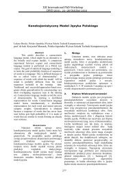
and voltages) can be controlled. In fig 16-18 static
characteristics of the controlled converter are shown.
Maximum input/output voltage transfer ratio by
325

sinusoidal current shape is below 1 what is shown in
fig. 16. In fig. 17 obtained range of input power
factor changes is shown. Coefficient efficiency for
presented MC is shown in fig. 18.
1
0.8
U L/ U S
0.6
Experiment: 50 Hz
Experiment: 75 Hz
0.4
Experiment: 25 Hz
Simulation: 50 Hz
0.2
Simulation: 75 Hz
0
0 0.1 0.2 0.3 0.4 0.5
q
Simulation: 25 Hz
0.6 0.7 0.8 0.9
Fig. 16. Input/output voltage ratio (UL/US) as a function
of desired in program Input/output voltage (q) for fL=25,
50, 75 Hz
0,9
0,8
0,7
0,6
0,5
0,4
0,3
0,2
q
0,2 0,4 0,6 0,8 1 0,8 0,6
Fig. 17.Input power factor changes as a function of
input/output voltage transfer ratio q dla for fL=25, 50, 75 Hz
1
?=P L/ P S
0,8
Fig. 18. Experimental efficiency coefficient as a function of
input/output voltage transfer ratio q dla for fL=25, 50, 75 Hz Hz
5. Conclusions
In this paper the project of the control
circuit of MC with implemented space vector
modulation and four step commutation strategy has
been presented. Simulation and experimental tests
results have confirmed that the presented control
technique exploits the MC’s possibility to control the
input power factor regardless of the output power
factor. In addition frequency and amplitude of the
output voltage can be controlled. Implementation of
the direct space vector modulation and four step
current commutation strategies for Matrix-
Reactance Frequency converter will be the subject of
investigation in the near future.
6. References
Inductive character Capacitive . character
f L
25 Hz
50 Hz
75 Hz
Sym. Exp. .
0,6
0,4
Experiment 50 Hz
Experiment 25 Hz
Experiment 75 Hz
0,2
0,1 0,2 0,3 0,4 0,5
q
0,6 0,7 0,8 0,9
[1] Venturini M., Alesina A., The generalized transformer: a new bidirectional
sinusoidal waveform frequency converter with
continuously adjustable input power factor, IEEE Power Electronics
Specialists Conference Record, PESC’80, pp. 242-252.
? p
326
[2] Alesina A., Venturini M., Analises and Design of Optimum-
Amplitude Nine-Switch Direct AC-AC Converters, IEEE
Transactions on Power Electronics, Vol. 4, no. 1, pp. 101-112, Styczeń
1989
[3] Ziogas P. D., Khan S. I. and Rashid M. H., Analysis and design of
forced commutated cycloconverer structures with improved
transfer characteristics, IEEE Trans. Ind. Electron., vol. IE-33, pp.
271-280, Aug 1986
[4] Huber L., Borojevic D., Space vector modulator for forced
commutated cycloconverters, in Conf. Rec. IEEE-IAS Annu.
Meeting, vol. 1, 1989, pp. 871-876
[5] Casadei G., Grandi G., Serra G., and Tani A., Space vector control
of matrix converters with unity input power factor and sinusoidal
input/output waveforms, in Proc. EPE Conf., vol. 7, Brighton, U.K,
Sept, 13-16, 1993, pp. 170-175
[6] Casadei D., Sierra G., Tani A., Reduction of the input current
harmonic content in matrix converters under input/output
unbalance, IEEE Trans. Ind. Electron., vol. 45, pp. 401-411, June
1998
[7] Blaabjerg F., Casadei D., Klumpner Ch., Matteini M.: Comparison
of Two Current Modulation Strategies for Matrix Converters
Under Unbalanced Input Voltage Conditions
[8] Casadei D., Serra G., Tani A, Zarri L., Matrix Converter
Modulation Strategies: A New General Approach Based on Space-
Victor Representation of the Switch State, IEEE Transactions on
Industrial Electronic, vol. 49, no. 2, pp. 370-381, April 2002
[9] Wheeler P. W., Rodriguez J., J. C. Clare, L. Empringham,
Weinstein A.: Matrix Converters: A Technology Reviev, IEEE
Transactions on Industrial Electronic, vol. 49, no. 2, pp. 276-387. April
2002.
[10] Tadra G., Fedyczak Z., Koncepcja układu sterowania dla
przekształtnika matrycowego z bezpośrednim sterowaniem
wektorowym Wiadomości Elektrotechniczne 10.2008, s. 18-21
[11] Casadei D., Trentin A., Matteini M., Calvini M., Matrix Converter
Commutation Strategy Using both Output Current and Input
Voltage Sign Measurement. EPE 2003.
[12] Zino v iev G. S., Obucho v A. Y., Ot chenasc h W. A.,
Popov W. I., Transformer less PWM AC boost and buck-boost
converters (In Russian), Technicznaja Elektrodinamika, T 2, pp.36-39.
Nac. Akademia Nauk Ukrainy, Kijev 2000.
[13] Fedyczak Z., Szcześn ia k P., Study of matrix-reactance
frequency converter with buck-boost topology, PELINCEC 2005,
(2005), CD-ROM.
[14] Fedyczak Z., Szcześni ak P., Klytta M., Matrix-reactance
frequency converter based on buck-boost topology, 12th Conf.
EPE-PEMC, (2006), 763-768, CD-ROM.
[15] Fedyczak Z., Szcześni ak P., K orotyeye v I., Generation of
matrix-reactance frequency converters based on unipolar matrixreactance
choppers, Proc. of PESC’08, (2008), 1821-1827.
[16] Fedyczak Z., Szcześniak P., Korotyeyev I., New family of matrixreactance
frequency converters based on unipolar PWM AC
matrix-reactance choppers, Proc. of EPE-PEMC 2008, pp. 236 –
242, Poznań 2008.
[17] Szcześniak P., Fedyczak Z., Klytta M., Modelling and analysis of a
matrix-reactance frequency converter based on buck-boost
topology by DQ0 transformation“, Proc. of EPE-PEMC 2008, pp.
165–171, Poznań 2008.
[18] K orotyeye v I.Y., Fed yczak Z., Steady and transient state
modelling methods of matrix-reactance converter with buck-boost
topology, COMPEL 28 (2009), n.3, 626 – 638.
[19] Fedyczak Z., Szcześniak P., Tadra G., Implementacja trójfazowych
przemienników częstotliwości bazujących na topologii matrycoworeaktancyjnego
sterownika prądu przemiennego typu buck-boost
SENE 2009, Łódź 2009 (Przyjęty do prezentacji).
[20] Gilles R., Goerges-Emile R.: “Direct Frequency Changer Operation
Under a New Scalar Control Algorithm” IEEE Transactions on Power
Electronics, Vol. 6, No. 1, January 1991, 100-107.
This work was supported by Polish Ministry of Science and
Higher Education, Project No. N510 036 32/3380
Pragnę serdecznie podziękować dr hab. inŜ. Zbigniewowi Fedyczakowi
prof. UZ, panu mgr inŜ. Pawlowi Sczesniakowi oraz panu Markowi
Szymankowi za pomoc w przygotowaniu powyŜszej pracy.
mgr inŜ. Tadra Grzegorz
Uniwersytet Zielonogórski
ul. Licealna 9
65-417 Zielona Góra
gtadra@iee.uz.zgora.pl