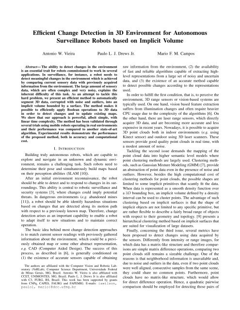
Efficient Change Detection in 3D Environment for Autonomous ...

Efficient Change Detection in 3D Environment for Autonomous
Surveillance Robots based on Implicit Volume
Antonio W. Vieira Paulo L. J. Drews Jr. Mario F. M. Campos
Abstract— The ability to detect changes in the environment
is an essential trait for robots commissioned to work in several
applications. In surveillance, for instance, a robot needs to
detect meaningful changes in the environment which is achieved
by comparing current sensory data with previously acquired
information from the environment. The large amount of sensory
data, which are often complex and very noisy, explains the
inherent difficulty of this task. As an attempt to tackle this
hard problem, we present an efficient method to automatically
segment 3D data, corrupted with noise and outliers, into an
implicit volume bounded by a surface. The method makes it
possible to efficiently apply Boolean operations to 3D data
in order to detect changes and to update existing maps.
We show that our approach is powerful, albeit simple, with
linear time complexity. The method has been validated through
several trials using mobile robots operating in real environments
and their performance was compared to another state-of-art
algorithm. Experimental results demonstrate the performance
of the proposed method, both in accuracy and computational
cost.
I. INTRODUCTION
Building truly autonomous robots, which are capable to
explore and navigate in an unknown and dynamic environment,
remains a challenging task. Such robots need to
determine their pose and simultaneously build maps based
on their perception abilities (SLAM [10]).
After an initial environment reconnaissance, the robot
should be able to detect and to respond to changes in its surroundings.
This ability is central to robotic surveillance and
security systems [3], where changes could imply potential
threats. In dangerous environments (e.g. abandoned mines
[11]), a robot should be able identify hazardous situations
based on changes that are detected along its motion path
with respect to a previously known map. Therefore, change
detection arises as an important capability to enable a robot
to adapt itself to new situations and to maintain correct
operation.
The basic idea behind most change detection approaches
is to match current sensor readings with previously gathered
information about the environment, which could be a previously
obtained map or some other abstract representation,
e.g. CAD (Computer Aided Design). The success of this
process, as described in [6], is generally conditioned on
(1) the existence of accurate sensors capable of obtaining
The authors are affiliated with the Computer Vision and Robotic Laboratory
(VeRLab), Computer Science Department, Universidade Federal
de Minas Gerais, MG, Brazil. Antonio W. Vieira is also affiliated with
CCET, UNIMONTES, MG, Brazil. Paulo L. J. Drews Jr is also affiliated
with C3, FURG, RS, Brazil. This work has been supported by grants
from CNPq, CAPES, FAURG and FAPEMIG. E-mails: {awilson,
paulol, mario}@dcc.ufmg.br
raw information from the environment, (2) the availability
of fast and reliable algorithms capable of extracting highlevel
representations from a large set of noisy and uncertain
data, and (3) the existence of an accurate method capable
to detect possible changes according to the representations
used.
In order to fulfill the first condition, that is, to perceive the
environment, 3D range sensors or vision-based systems are
typically used. On one hand, vision based feature extraction
suffers from illumination changes and often require heavier
CPU usage due to the complexity of the algorithms [6]. On
the other hand, there are laser range sensors, which directly
acquire 3D data, and are becoming more accurate and less
expensive in recent years. Nowadays, it is possible to acquire
3D point clouds both in indoor environments (e.g. using
Kinect sensor) and outdoor using 3D laser scanners. These
sensors provide good quality point clouds in real time, with
a modest amount of noise.
Tackling the second issue demands the mapping of the
point cloud data into higher semantic level models where
point clustering methods are largely used. Clustering methods,
such as Gaussian Mixture Modeling (GMM) [7], provide
an abstraction of point data even in the presence of noise and
outliers. However, besides the high computational cost of
clustering methods for point clouds, the possible shapes are
limited to some implicit primitives that scantly fit the data.
When data is represented as a smooth density function over
a 3D bounding box, an implicit volume defined by a density
interval can be used to cluster points. The advantage of such
clustering based on implicit surfaces is that the shape of
implicit objects are not limited to any specific primitive, but
are rather flexible to describe a fairly broad range of objects
with respect to their geometry and topology. [9] presents a
hierarchical clustering method based on implicit surfaces that
are suited for visualization of large datasets.
Finally, concerning the third issue, several metrics have
been proposed to detect changes using data acquired by
the sensors. Differently from intensity or range images, for
which data has a matrix-like structure and therefore comparisons
are simple matrix difference operations, comparing two
point clouds still remains a sizeable challenge. One of the
reasons is that neighborhood information is unavailable and,
due to noise and outliers in the data, even if two point clouds
were well aligned, consecutive samples from the same scene,
they could share no common points. Furthermore, point
clouds have no matrix-like structure, which would allow
for direct difference operation. Hence, a quadratic pairwise
comparison should be employed for detecting those pairs of

points whose distance is less than a given threshold.
In order to reduce the computational cost of this process,
more complex metrics have been used, which include
statistical information associated to the underlying point
distributions. The main disadvantage of this kind of approach
is its strong dependence on the number of distributions
associated with the map.
In this work, we propose to use point clouds to build
a density function over a 3D bounding box by fitting a
local density function to each point and summing these
functions into an accumulated global density function. This
global density function is used to directly extract a boundary
surface that summarizes the data within a density interval.
This leads to a clustering strategy that has several important
advantages: (1) It is robust to noise and outliers, (2) provides
a high semantic level model which allows for Boolean set
operations over different point clouds, and (3) it is efficient
as far as time complexity is concerned. Fig. 1 illustrates
the proposed approach, where the red dashed boxes, on the
left, represent a prior data; the acquired data is shown in
continuous blue boxes, in the middle; and the input-output
is shown in black boxes, on the right.
Fig. 1. Problem statement: Given 3D data acquired by a robot and a
known map on the environment, the robot detects and segments changes in
the scene using implicit clusters and Boolean operations.
The remainder of the paper is organized as follows: Sec. II
briefly reviews related works. Sec. III describes our change
detection approach. Experimental results are shown in Sec.
IV and, finally, Sec. V presents the conclusions and future
work directions.
II. RELATED WORK
In the last decade, the behavior of an autonomous mobile
robot working in dynamic environments has been intensively
studied. In order to tame the complexity of the problem,
several approaches have typically used as the main strategy
to ignore dynamic objects from the modeling process in order
to improve navigation and localization tasks [10]. However,
these changes in the robot’s surroundings may actually be
relevant depending on the application. Following this idea,
Andreasson et al. [1] presented a system for autonomous
change detection with a security patrol robot using 3D laser
range data and, unlike our approach, they also used images
from a color camera.
Change detection, in the context of surveillance robots,
was also addressed in the work of Vieira Neto and Nehmzow
[12], where they compare the use of self-organizing maps
with incremental PCA in order to model the world and
identify changes therein. Differently from the work that we
present in this paper, they applied their method to visual
colored data, where visual attention was employed based on
salience maps.
Kaestner et al. [4] presented a method based on “difference
image” where a probabilistic approach is used for alignment
and change detection using range sensor data. Their alignment
method provides a non-rigid point cloud registration to
deal with estimation errors and changes between datasets are
detected using a probabilistic threshold to recognize changes.
However, robustness and performance are not discussed.
A combination of Gaussian Mixture Model (GMM) and
the Earth Mover’s Distance(EMD) algorithms was proposed
by Drews et al. [3] in order to detect changes in raw 3D point
clouds. Furthermore, they retrieved superquadric shapes from
changes, in order to classify the encountered changes. In spite
of the impressive results attained, the computation time of the
proposed techniques were not suitable for large datasets. This
was mainly due to the use of the Expectation Maximization
algorithm to retrieve GMMs. That work was extended in
Núñez et al. [6], where the structural matching algorithm
was used instead of EMD to determine changes in GMM
space. In spite of the limited number of tests they conducted,
the results showed that the new approach represented an
improvement in terms of computational cost and sensitivity
to the number of Gaussians needed for the representation.
The main limitation of using 3D raw point clouds to
detect changes is related to the clustering of data without
the knowledge of surface normals and neighborhood information.
The notion of neighborhood of a point in a point
cloud subjectively suggests the idea of connectivity.
In this work, we introduce a method based on implicit
functions [2] to extract a boundary surface that clusters the
point cloud, allowing efficient change detection, Boolean
operations and segmentation. Differently from [13], where
a signed distance field is used to obtain an implicit surface
fitting the data points at zero level, our goal is to define a
level surface to cluster data points.
III. METHODOLOGY
In this section, we detail how to build our global density
function from a point cloud set and how to use the implicit
function theorem to define a surface that clusters points according
to spatial density values. Finally, Boolean operations
over two point clouds is presented using its corresponding
density functions.
A. Density Function from Point Cloud
The main idea of our method is to estimate an unknown
global density function G : R 3 → R from a given point cloud
P = {(xi, yi, zi) , 1 ≤ i ≤ n} such that larger values occurs
in points close to the surface where P was sampled. This
global density function should define a continuous smooth

scalar field over which an isovalue density threshold h can
be used to cluster points in the implicit volume defined by
the set S = {p ∈ R 3 ; G (p) ≥ h}.
Given a point cloud set P with n points, we define, for
each point pi ∈ P , a simple local density gi : R 3 → R which
is a kernel function chosen to be a Gaussian:
gi (p) = exp
.
− pi−p2
2σ 2
The parameter σ smooths the influence of pi over its
neighborhood. We set σ with the value of the maximum
Euclidean distance from two points pi, pj ∈ P to be
considered neighbors. Hence, if pi and pj are neighbors,
which means pi − pj ≤ σ, the density contribution δ
between pi and pj is given by
δ = gi (pj) = e − pi−pj 2
2σ2 1 − ≥ e 2 .
In order to define the global density function G, we
accumulate the local density functions gi contributed by all
points pi, 1 ≤ i ≤ n,
n
G (p) = gi (p).
i=1
Since the local density function gi (pi) = 1 for all pi ∈ P ,
if pi has k neighbors, then G (pi) ≥ 1 + kδ. Our method
clusters only points with k or more neighbors by setting a
threshold value h = 1 + kδ. Fig. 2 and 3 illustrates this
clustering strategy for 1D and 2D point cloud, respectively.
Fig. 2. Example of the point clustering in 1D. Local density functions are
accumulated to define a global density function. Notice that accumulated
density for p5 is insufficient to cluster it, given the threshold.
(a) (b) (c)
Fig. 3. Example of the point clustering in 2D. Increasing values of
smoothing parameter σ, lead to increasing cluster volume and more points
are clustered. In (a), two points are considered outliers, in (b) only one point
is considered outliers and, in (c), no outliers is considered.
In order to speed up computation, we obtain a discrete
sampling for the global density function by computing its
values for a 3D grid defined for the bounding box of the
point cloud P . For each point pi ∈ P , its local density
contribution is calculated and summed only for a constant
number of grid points on its neighborhood according to the
kernel mask size s. So, the global density function G is
sampled, for all points on the grid, in time O (n) for a point
cloud with n points. The grid values is used as a discrete
approximation for G.
B. Clustering by Implicit Surface
From the theorem of implicit functions, we have that if
f : R 3 → R is smooth and h ∈ R is a regular value, that is,
∇f (p) = 0 for all p ∈ f −1 (h), then f −1 (h) is a surface
that partitions the domain R 3 into three sets:
S1 = {p ∈ R 3 ; f(p) < h},
S2 = {p ∈ R 3 ; f(p) = h},
S3 = {p ∈ R 3 ; f(p) > h}.
The global density function G constructed as described
in the previous section is a smooth scalar function in R 3
and setting a constant threshold h > 1, we define a surface
S2 ⊂ R 3 as the boundary of a continuous volume region
that clusters the point set P . Setting h = 1 + kδ we define
a set to cluster points that have at least k neighbors whose
distance is less or equal than σ. This set is implicitly defined
as S = {p ∈ R 3 ; G (p) > h}.
In order represent and visualize the set S, we extract
a piecewise linear boundary surface for this cluster using
the algorithm Marching Cubes [5]. The method Marching
Cubes produces a mesh of triangles approximating the preimage
G −1 (h) from a grid of cubes where the values of the
function G are known at its vertices. Each cube vertex on the
grid is classified either as positive or as negative, according
to its relative position with respect to the set S. The resulting
mesh represents a boundary surface that clusters the raw
point cloud. Different level sets can be extracted for the same
point cloud as long as we use a different isovalue h.
Figure 4-a shows an example of a point cloud with some
outliers; its level set surface extracted for a global density
value h = 1 + 2δ is depicted in Figure 4-b, and another
level set surface extracted for density level h = 1 + 3δ is
shown in Figure 4-c. Notice that multiple components are
well clustered. Notice, also, that in Figure 4-c the higher
density level clustering leads to a disconnected component
(a) (b) (c)
Fig. 4. Example of the point cloud clustering in 3D. Raw point cloud (a),
the clustering set for density level h = 1 + 2δ (b) and the clustering set for
density level h = 1 + 3δ (c).

for the person’s head and that in the lower members, a hole
appeared separating the two legs.
Given a threshold h, we will consider a normalized global
density function G(p) = h − G(p), where zero value defines
the boundary surface, negative and positive values define
interior and exterior regions of the cluster, respectively. The
use of G allows, without loss of generality, for the efficient
use of Boolean operations on implicit volumes.
C. Boolean Operations
Let two point clouds P1 and P2 represent current and
reference data, respectively. It is hard to perform Boolean
operations such as P1 ∩ P2 or P1 − P2. However, using
their associated normalized global density functions, given
by G1, G2 : R 3 → R, each Boolean operation constructs a
new normalized global density function G3 in a simple step,
as shown in [8], using the following operations:
P1 ∪ P2 ⇒ G3 (p) = min (G1 (p) , G2 (p))
P1 ∩ P2 ⇒ G3 (p) = max (G1 (p) , G2 (p))
P1 − P2 ⇒ G3 (p) = max (G1 (p) , −G2 (p))
The above Boolean operation is defined for implicit data
only. In order to take advantage of this procedure to compute
changes from our discrete point clouds, we obtain
G3 (p) = max (G1 (p) , −G2 (p)), which is a new density
function whose negative values define a volume where points
belonging to the portion where there is a change should lie.
Finally, points p ∈ P1 are detected as a change if G3(p) < 0,
which is computed in linear time. Figure 1 shows an example
of an operation of difference between two point clouds.
Algorithm 1 details our method.
Algorithm 1 ChangeDetect( P1, P2, h )
1: Compute G1 from P1
2: Compute G2 from P2
3: Compute G3 = max(G1, −G2)
4: D = ∅
5: for each p ∈ P1 do
6: if G3(p) < 0 then
7: D = D ∪ {p}
8: end if
9: end for
10: return D
Notice that, as it is, Algorithm 1 computes change points
that shows up. Disappearing change points can be computed
as well by swapping P1 and P2 in the input.
IV. EXPERIMENTAL RESULTS
In order to obtain statistical quantitative assessment of
the proposal method, we use the methodology proposed by
Vieira Neto and Nehmzow [12] to evaluate change detection.
They propose the use of contingency tables to relate the
system response with ground truth information to obtain
three different statistical indicators based on χ 2 analysis. In
our work, the ground truth data was manually segmented by
the authors.
Vieira Neto and Nehmzow propose the use of three
metrics: Cramer’s V , uncertainty coefficient U(0 ≤ V, U ≤
1) and κ index of agreement. Those methods were used
to quantify the strength of data association, where small
values indicate weaker associations and values closer to one
represent stronger associations. The index κ varies between
[−1; 1], where values smaller than 0.1 indicate no agreement,
values between 0.1 and 0.4 indicate a weak agreement,
values between 0.4 and 0.6 indicate a clear agreement and
values larger than 0.6 indicate a strong agreement.
Due to the similarity between these metrics, we show only
the κ index of agreement in order to show the accuracy of
our method. The κ index can be computed using Equation
1, where A represents inliers, B represents detection failure,
C represents outliers, and D represents correct detection of
the absence of change. More details on these metrics can be
found in [12].
κ =
2(AD − BC)
(A + C)(C + D) + (A + B)(B + D)
A. Evaluation of robustness and parameters sensitivity
The experiments to evaluate robustness of our method used
a 3D dataset acquired in an office environment as reference
map and 10 different datasets of the same environment
modified with objects of different sizes and shapes. A Pioneer
2-AT Robot equipped with a Microsoft Kinect sensor was
used to obtain the data, and each data set has about 76k
points. The environment and 10 different changes are shown
in Fig. 5-a and 5-b. The tests were executed on a PC with a
Core 2 Duo CPU running at 2.0 GHz and with 2 GB RAM.
Our algorithm obtains a discrete sampling for the global
density function by computing its values for a 3D grid
defined for the bounding box of the point clouds. Larger grid
size leads to dense sampling, which improves robustness but
decreases performance, as shown in Fig. 6. Firstly, Fig. 6-a
depicts the statistical results using the κ index with mean and
standard deviation (error bar). These results were generated
on a grid 40 × 40 × 40 to 320 × 320 × 320, with a step
of 40. The result shows that high accuracy is obtained from
grid size 120 × 120 × 120 and that this accuracy is stable for
higher values. Considering values greater than 0.6 as good
(a) (b)
Fig. 5. Experimental Setup 1: (a) Environment and experimental setup
composed of a Pioneer Robot equipped with a Kinect sensor used to acquire
3D data. (b) Ten different changes inserted in the office environment, with
varies size, pose and shape.
(1)

TABLE I
COMPARATIVE STUDY OF DIFFERENT CHANGE DETECTION ALGORITHMS.
Number of Points Build Ref. Map Build Cur. Map Detection
Dataset Ref. Map Cur. Map Nuñez et al. Our Nuñez et al. Our Nuñez et al. Our
Real Data - Test Area 1 79171 79633 177.21 1.12 164.56 1.07 0.014 0.146
Real Data - Test Area 2 79171 81134 177.36 1.16 110.86 1.05 0.014 0.149
Real Data - Test Area 3 79171 80112 167.88 1.14 109.22 1.06 0.028 0.166
detection, we are able to detect changes even for small sized
changes (see Figure 5-b).
Figure 6-b, shows the processing time of the proposed
algorithm. The processing time is obtained considering the
total time for each of the three steps: (1) building implicit
volume for reference point cloud, (2) building implicit volume
for the point cloud with changes and, (3) performing
the Boolean operation (change detection). The results are
shown with mean time and standard deviation. This graph
shows that increasing grid size, increases computational time
without any gain in accuracy for grid sizes greater than
80 × 80 × 80, for which high accuracy is obtained in less
than half a second.
(a)
(b)
Fig. 6. Results obtained using different datasets acquired with the Kinect
device, with objects of different sizes and shapes and for different poses.
a) The statistical assessment κ index of agreement for grid size changes. b)
Processing time for each dataset change in the grid size.
In order to experimentally show the linear time complexity
of our method, we computed changes for point clouds with
different sizes. For this experiment, nine sets were used for
which the number of points varyed from 17k to 144k. For
each dataset, five different acquisitions were processed to
Fig. 7. Computation time for different point cloud sizes. Nine sets
with different sizes from 17k to 144k were used to show the linear time
complexity in the number of points.
present the mean and standard deviation of the processing
time as shown in Figure 7.
B. Comparison with a state-of-art approach
We use compare our method with the one presented in [6]
on their dataset. That dataset was acquired in the hallways
of a building of the Minas Gerais Federal University using
a Pioneer 2-AT Robot equipped with two SICK LMS-200
mounted orthogonally, in order to localize and acquire 3D
maps. For the experiments, three different novelties were
included in the robot’s workspace: An identification cylinder,
a person and a printer box. The environment and the objects
used are shown in Fig. 8-a and 8-b.
Considering the results shown in [6], we are able to
compare only the processing time. The accuracy of the
method is not available because different metrics were used
in the evaluation processes of each method. As in [6], we
are also capable to detect changes in all three scenarios,
(a) (b)
Fig. 8. Experimental Setup 2: (a) Environment and experimental setup composed
of a Pioneer 2-AT Robot equipped with two orthogonally mounted
laser scanners acquiring 3D data. (b) Three different changes were inserted
in the robot’s environment.

albeit faster. Table I uses the best times obtained in the
work of Nuñez et al. [6]. Both methods are divided into two
steps, where the first step builds a “special” representation
and the second step compares this representation (called
Detection). In the case of [6], the representation is built using
a simplification method and GMM estimation. In our method,
the representation tailored to building implicit volumes. The
change detection is achieved using structural matching in [6],
and Boolean operation in our approach.
Notice that, for all datasets, our method is substantially
faster to build the required representation. The main limitation
of the method proposed by Nuñez et al. [6] is related
to the Gaussian Mixture Models using the Expectation-
Maximization algorithm, which has lower computational performance
and is quite sensitive to the number of Gaussians,
which is one of the parameters of the EM algorithm.
Besides the improvement in computational time processing,
we empirically observe, from other results as shown
in the Figure 9, that our method performs quite robustly in
the presence of parallax and highly complex geometry. In
the work of [6], the datasets obtained by the robot show
the walls and some objects, but the roof was also acquired,
where pipes and other objects are present in the ceiling, as
shown in Figure 8-a. However, this data are not considered
in their experiment, because of to the high data complexity
due parallax and absence of meaningful changes. In another
experiment, we used the “complete” information available
from this dataset to describe the data including all the points.
Figure 9-a shows one example of “complete” point cloud
obtained using the Pioneer robot (see Fig. 8-a) where one
person produce the change (see Fig. 8-b). The blue dots
represent the points detected as not change, and the red points
as change points detected by our algorithm. Some red points
are in the ceiling, and this is due to the parallax effect in
the acquisition and misalignment between reference dataset
(without change) and the present dataset (with change).
Figure 9-b shows the clustered volume obtained with our
implicit approach for the complete dataset. The point cloud
is approximately twice as large as the partial volume, i.e. it
has approximately 150k points. We were able to correctly
detect changes for this dataset in less than one second.
V. CONCLUSIONS AND FUTURE WORK
This paper described a novel method to detect changes in
a 3D real environment for robot navigation. Results obtained
with two different experimental platforms are shown. A new
approach to detect changes based on implicit volumes allow
us to detect changes using Boolean operation. It enables us to
localize the existence of novelties in the scene, i.e. segment
them. Results of the proposed algorithm demonstrate the
reliability and efficiency of the approach. The algorithm
was compared with a state-of-art approach and obtained
substantially better results in terms of computational cost
and similar as far as detection and accuracy are concerned.
Future investigation will focus on the extension of the
method to work iteratively, with the data being captured
online by the robot. Another important improvement is to
(a) (b)
Fig. 9. Change detection algorithm comparison: a) example of point cloud
obtained using Pioneer robot (see Fig. 8-a) with one person as change (see
Fig. 8-b). Changes detected by the algorithm is indicated by red points,
where is possible to see some outliers in the roof. b) Implicit volumes
obtained from point cloud in a) generated by our approach.
perform the registration between clouds concurrently with
Boolean operation. This will ultimately allow us to correlate
and align similar points and obtain good registration even
for significant changes in environmental and acquisition
conditions.
REFERENCES
[1] Henrik Andreasson, Martin Magnusson, and Achim J. Lilienthal. Has
something changed here? autonomous difference detection for security
patrol robots. In Proc. IROS, pages 3429–3435, San Diego, USA,
2007.
[2] Jules Bloomenthal and Brian Wyvill, editors. Introduction to Implicit
Surfaces. Morgan Kaufmann Publishers Inc., San Francisco, CA, USA,
1997.
[3] Paulo Drews Jr, P. Núñez, R. Rocha, M. Campos, and J. Dias. Novelty
detection and 3d shape retrieval using superquadrics and multi-scale
sampling for autonomous mobile robots. In Proc. ICRA, pages 3635–
3640, may 2010.
[4] Ralf Kaestner, Sebastian Thrun, Michael Montemerlo, and Matt Whalley.
A non-rigid approach to scan alignment and change detection
using range sensor data. In FSR, pages 179–194, 2005.
[5] Thomas Lewiner, Hélio Lopes, Antônio Wilson Vieira, and Geovan
Tavares. Efficient implementation of marching cubes cases with
topological guarantees. JGT, 8(2):1–15, december 2003.
[6] P. Núñez, P. Drews, A. Bandera, R. Rocha, M. Campos, and J. Dias.
Change detection in 3d environments based on gaussian mixture model
and robust structural matching for autonomous robotic applications. In
Proc. IROS, pages 2633 –2638, oct. 2010.
[7] P. Núñez, P. Drews, R. Rocha, M. Campos, and J. Dias. Novelty
detection and 3d shape retrieval based on gaussian mixture models
for autonomous surveillance robotics. In Proc. IROS, pages 4724–
4730, Piscataway, NJ, USA, 2009. IEEE Press.
[8] A. Ricci. A constructive geometry for computer graphics. The
Computer Jornal, 16(2):157–160, 1973.
[9] T. C. Sprenger, R. Brunella, and M. H. Gross. H-blob: a hierarchical
visual clustering method using implicit surfaces. In In Proc. VIS, pages
61–68, Los Alamitos, CA, USA, 2000. IEEE Computer Society Press.
[10] Sebastian Thrun, Wolfram Burgard, and Dieter Fox. Probabilistic
Robotics. The MIT Press, 2005.
[11] Sebastian Thrun, Dirk Hahnel, David Ferguson, Michael Montemerlo,
Rudolph Triebel, Wolfram Burgard, Christopher Baker, Zachary Omohundro,
Scott Thayer, and William Whittaker. A system for volumetric
robotic mapping of abandoned mines. In Proc. ICRA, pages 4270–
4275, 2003.
[12] Hugo Vieira Neto and Ulrich Nehmzow. Visual novelty detection for
autonomous inspection robots. In Yoshihiko Takahashi, editor, Service
Robot Applications, pages 309–330. I-Tech Education and Publishing,
Vienna, Austria, 2008.
[13] Weihong Wang Xujia Qin and Qu Li. Practical boolean operations on
point-sampled models. In Proc. ICCSA, 3980:393–401, 2006.