- Page 1 and 2:
LOW-MASS X-RAY BINARIES, DIFFUSE GA
- Page 3 and 4:
smaller GCs are more likely to cont
- Page 5 and 6:
GO2-3099X, GO3-4099X, AR3-4005X, GO
- Page 7 and 8:
her room (my apologies to her offic
- Page 9 and 10:
US Court expert from India), for al
- Page 11 and 12:
Table of contents Abstract ii Ackno
- Page 13 and 14:
5.2.1 Chandra X-ray Observatory . .
- Page 15 and 16:
List of Figures 1.1 Hubble Tuning F
- Page 17 and 18:
List of Tables 1.1 Galactic Low-Mas
- Page 19 and 20:
Chapter 1 General Introduction 1.1
- Page 21 and 22:
Fig. 1.1.— Hubble Tuning Fork, co
- Page 23 and 24:
2000). In most HMXBs, the accreted
- Page 25 and 26:
not get a complete picture of the L
- Page 27 and 28:
this, the result of dynamical inter
- Page 29 and 30:
is the Advanced CCD Imaging Spectro
- Page 31 and 32:
Chapter 2 Chandra Observations of L
- Page 33 and 34:
keV (Sarazin et al. 2000, 2001). Wi
- Page 35 and 36:
agreed with positions from the USNO
- Page 37 and 38:
24:00 22:00 7:20:00 18:00 16:00 18:
- Page 39 and 40:
Table 2.1. Discrete X-ray Sources i
- Page 41 and 42:
Table 2.1—Continued Source d Coun
- Page 43 and 44:
Table 2.2. Discrete X-ray Sources i
- Page 45 and 46:
Table 2.2—Continued Source d Coun
- Page 47 and 48:
optical/IR positions of R.A. = 12 h
- Page 49 and 50:
log N(>L) 2.0 1.5 1.0 0.5 0.0 NGC 4
- Page 51 and 52:
luminosity function for luminositie
- Page 53 and 54:
H31 1.0 0.5 0.0 -0.5 -1.0 NGC 4365
- Page 55 and 56:
2.4.5 Variability We searched for v
- Page 57 and 58:
Number 10 8 6 4 2 NGC 4365 Optical
- Page 59 and 60:
LMXBs has an effective radius of 12
- Page 61 and 62:
component (“MEKAL”) was used fo
- Page 63 and 64:
Table 2.4. X-ray Spectral Fits of N
- Page 65 and 66:
Fig. 2.9.— Top panels: Cumulative
- Page 67 and 68:
we extended the spectrum down to 0.
- Page 69 and 70:
We also examined whether the unreso
- Page 71 and 72:
esolved sources in the galaxy. This
- Page 73 and 74:
temperature ∼0.3 keV. Matsumoto e
- Page 75 and 76:
log I X (counts/sec/arcmin 2 ) -1.0
- Page 77 and 78:
∼45% of the counts are resolved i
- Page 79 and 80:
Chapter 3 Chandra Observations of D
- Page 81 and 82:
noninteracting members (de Vaucoule
- Page 83 and 84:
used for spectroscopic analysis. We
- Page 85 and 86:
02:00.0 03:00.0 04:00.0 05:00.0 06:
- Page 87 and 88:
Table 3.1. Discrete X-ray Sources i
- Page 89 and 90:
Table 3.1—Continued d a Count Rat
- Page 91 and 92:
We also attempted detections in mul
- Page 93 and 94:
sociated with extended X-ray or opt
- Page 95 and 96:
Fig. 3.3.— Histogram of the obser
- Page 97 and 98:
chip. The number of ULX candidates
- Page 99 and 100:
these luminosities among previously
- Page 101 and 102:
to 2-6 keV. Since the 6-10 keV rang
- Page 103 and 104:
absorption and varying power-law in
- Page 105 and 106:
counts occur within ∼ 4 ks. Sourc
- Page 107 and 108:
log I X (counts/sec/arcmin 2 ) 0.5
- Page 109 and 110:
tion), and βouter = 0.36 +0.01 −
- Page 111 and 112:
the east and northeast of NGC 1600.
- Page 113 and 114:
group, we assumed that they were at
- Page 115 and 116:
the group gas than we calculate fro
- Page 117 and 118:
04:55 -5:05:00 05 -5:05:10 15 -5:05
- Page 119 and 120:
for the spectrum: “Field” impli
- Page 121 and 122:
90% confidence level errors. Bracke
- Page 123 and 124:
we adopted the power-law model as o
- Page 125 and 126:
sources could be a non-trivial sour
- Page 127 and 128:
jection to include the emission fro
- Page 129 and 130:
Fig. 3.13.— Estimated gas and gra
- Page 131 and 132:
ackground source population cannot
- Page 133 and 134:
NGC 1600 that has a small spatial s
- Page 135 and 136:
(HMXBs). LMC X-4, an HMXB pulsar, h
- Page 137 and 138:
searched for the shortest time tn o
- Page 139 and 140:
with NGC 4697. Columns (1)-(4) list
- Page 141 and 142:
duration, ∆tflat, beginning at a
- Page 143 and 144:
the uncertainties quoted do not inc
- Page 145 and 146:
to persistent rate for short flares
- Page 147 and 148: Chapter 5 Multi-Epoch Chandra X-ray
- Page 149 and 150: the field, these different populati
- Page 151 and 152: luminous (MB < −20) elliptical (E
- Page 153 and 154: Although Chandra is known to encoun
- Page 155 and 156: 42:00.0 44:00.0 46:00.0 48:00.0 -5:
- Page 157 and 158: Fig. 5.3.— Adaptively smoothed Ch
- Page 159 and 160: 1 × 10 −5 count s −1 arcsec
- Page 161 and 162: Table 5.1—Continued Source R.A. D
- Page 163 and 164: Table 5.1—Continued Source R.A. D
- Page 165 and 166: Table 5.1—Continued Source R.A. D
- Page 167 and 168: source list against which to regist
- Page 169 and 170: ate from Observation 0784 alone (Pa
- Page 171 and 172: Table 5.2. : Optical Properties of
- Page 173 and 174: actually be an AGN. Sources 79, 80,
- Page 175 and 176: two potential GC counterparts. We l
- Page 177 and 178: Table 5.3—Continued X-ray Source
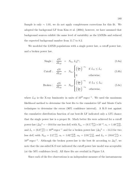
- Page 179 and 180: Fig. 5.6.— Color (G475−Z850) -
- Page 181 and 182: mass segregation of GCs with the sa
- Page 183 and 184: Table 5.4. Fits to the Expected Num
- Page 185 and 186: dependence are allowed to vary. Var
- Page 187 and 188: NGC 4697 to convert the observed so
- Page 189 and 190: Table 5.6—Continued Source LA LB
- Page 191 and 192: Table 5.6—Continued Source LA LB
- Page 193 and 194: Table 5.7. Combined Luminosities &
- Page 195 and 196: Table 5.7—Continued Source Not De
- Page 197: Fig. 5.8.— Cumulative luminosity
- Page 201 and 202: Fig. 5.10.— Cumulative luminosity
- Page 203 and 204: Fig. 5.11.— Merged luminosities (
- Page 205 and 206: Fig. 5.12.— X-ray color-color dia
- Page 207 and 208: 5.9 Spectral Analysis We performed
- Page 209 and 210: some data loss, it allows for direc
- Page 211 and 212: for 2 dof and the f-test indicates
- Page 213 and 214: ple to LMXBs interior to that semi-
- Page 215 and 216: est-fit (χ 2 = 56.4 for 65 dof) by
- Page 217 and 218: 5.10.1 Intraobservation Variability
- Page 219 and 220: Fig. 5.14.— Binned lightcurve usi
- Page 221 and 222: Table 5.10. Possible Flaring Source
- Page 223 and 224: Fig. 5.16.— Cumulative lightcurve
- Page 225 and 226: pairs of observations. In Figure 5.
- Page 227 and 228: Table 5.11—Continued Source PL,AB
- Page 229 and 230: Fig. 5.17.— Percentage of Analysi
- Page 231 and 232: dofs and the number of combinations
- Page 233 and 234: Table 5.12—Continued Source Obs.S
- Page 235 and 236: of states as transient candidates.
- Page 237 and 238: Long-Term Hardness Ratio Variabilit
- Page 239 and 240: In the final observation, there wer
- Page 241 and 242: limits). The 0.3-10 keV X-ray lumin
- Page 243 and 244: atio is expected only from the most
- Page 245 and 246: eak (Kim et al. 2006a). We find mar
- Page 247 and 248: LMXBs in Galactic GCs (Heinke et al
- Page 249 and 250:
in the field of the Milky Way and a
- Page 251 and 252:
6.2 Sample 6.2.1 Galaxy Sample Tabl
- Page 253 and 254:
Table 6.2. Properties of Chandra Ob
- Page 255 and 256:
identification of point sources, AC
- Page 257 and 258:
the QE degradation in the ACIS dete
- Page 259 and 260:
Table 6.3—Continued Galaxy NX LX,
- Page 261 and 262:
The positions of the GCs were used
- Page 263 and 264:
Fig. 6.2.— Scatter plot of GC gal
- Page 265 and 266:
Fig. 6.3.— Scatter plot of estima
- Page 267 and 268:
Fig. 6.5.— Scatter plot of estima
- Page 269 and 270:
isophote from the galaxy optical su
- Page 271 and 272:
6.3.1 Luminosity and Mass Prior obs
- Page 273 and 274:
compare their χ 2 fits to test whi
- Page 275 and 276:
GCs without LMXBs; however, there a
- Page 277 and 278:
following dependence on GC properti
- Page 279 and 280:
of this probability with individual
- Page 281 and 282:
Fig. 6.9.— Identical to Figure 6.
- Page 283 and 284:
We used the indices from our best-f
- Page 285 and 286:
(20.3 for half-mass radius, both wi
- Page 287 and 288:
most are steeper than Z ∼0.4 . Ei
- Page 289 and 290:
Fig. 6.11.— (Left:) Two-dimension
- Page 291 and 292:
differently by the properties of th
- Page 293 and 294:
dependent IMF (Grindlay 1987), or e
- Page 295 and 296:
a 1.4M⊙ neutron star (NS). They s
- Page 297 and 298:
equivalent to a dependence on the b
- Page 299 and 300:
variability timescale, but it is no
- Page 301 and 302:
7.2.1 X-ray Properties of the GC-LM
- Page 303 and 304:
of the metallicity dependence. As i
- Page 305 and 306:
Appendix A Encounter Rate Parameter
- Page 307 and 308:
Fig. A.1.— Dimensionless quantity
- Page 309 and 310:
and four; these positions do not in
- Page 311 and 312:
Table B.1—Continued RA Dec. d GC
- Page 313 and 314:
Table B.1—Continued RA Dec. d GC
- Page 315 and 316:
Table B.2. Optical Properties of Gl
- Page 317 and 318:
Table B.2—Continued RA Dec. d GC
- Page 319 and 320:
Table B.2—Continued RA Dec. d GC
- Page 321 and 322:
Table B.2—Continued RA Dec. d GC
- Page 323 and 324:
Table B.2—Continued RA Dec. d GC
- Page 325 and 326:
Table B.2—Continued RA Dec. d GC
- Page 327 and 328:
Table B.2—Continued RA Dec. d GC
- Page 329 and 330:
Table B.2—Continued RA Dec. d GC
- Page 331 and 332:
Table B.2—Continued RA Dec. d GC
- Page 333 and 334:
Table B.2—Continued RA Dec. d GC
- Page 335 and 336:
Table B.2—Continued RA Dec. d GC
- Page 337 and 338:
Table B.2—Continued RA Dec. d GC
- Page 339 and 340:
Table B.2—Continued RA Dec. d GC
- Page 341 and 342:
Table B.2—Continued RA Dec. d GC
- Page 343 and 344:
Table B.2—Continued RA Dec. d GC
- Page 345 and 346:
Table B.2—Continued RA Dec. d GC
- Page 347 and 348:
Table B.2—Continued RA Dec. d GC
- Page 349 and 350:
Table B.2—Continued RA Dec. d GC
- Page 351 and 352:
Table B.2—Continued RA Dec. d GC
- Page 353 and 354:
Table B.2—Continued RA Dec. d GC
- Page 355 and 356:
Table B.2—Continued RA Dec. d GC
- Page 357 and 358:
Table B.2—Continued RA Dec. d GC
- Page 359 and 360:
Table B.2—Continued RA Dec. d GC
- Page 361 and 362:
Table B.2—Continued RA Dec. d GC
- Page 363 and 364:
Table B.2—Continued RA Dec. d GC
- Page 365 and 366:
Table B.2—Continued RA Dec. d GC
- Page 367 and 368:
Table B.2—Continued RA Dec. d GC
- Page 369 and 370:
Table B.2—Continued RA Dec. d GC
- Page 371 and 372:
Table B.2—Continued RA Dec. d GC
- Page 373 and 374:
Table B.2—Continued RA Dec. d GC
- Page 375 and 376:
Table B.2—Continued RA Dec. d GC
- Page 377 and 378:
Table B.2—Continued RA Dec. d GC
- Page 379 and 380:
Table B.2—Continued RA Dec. d GC
- Page 381 and 382:
Table B.2—Continued RA Dec. d GC
- Page 383 and 384:
Table B.2—Continued RA Dec. d GC
- Page 385 and 386:
Table B.2—Continued RA Dec. d GC
- Page 387 and 388:
Table B.2—Continued RA Dec. d GC
- Page 389 and 390:
Table B.2—Continued RA Dec. d GC
- Page 391 and 392:
Table B.2—Continued RA Dec. d GC
- Page 393 and 394:
Table B.2—Continued RA Dec. d GC
- Page 395 and 396:
Table B.2—Continued RA Dec. d GC
- Page 397 and 398:
Table B.2—Continued RA Dec. d GC
- Page 399 and 400:
Table B.2—Continued RA Dec. d GC
- Page 401 and 402:
Table B.2—Continued RA Dec. d GC
- Page 403 and 404:
Table B.2—Continued RA Dec. d GC
- Page 405 and 406:
Table B.2—Continued RA Dec. d GC
- Page 407 and 408:
Table B.2—Continued RA Dec. d GC
- Page 409 and 410:
Table B.2—Continued RA Dec. d GC
- Page 411 and 412:
Table B.2—Continued RA Dec. d GC
- Page 413 and 414:
Table B.2—Continued RA Dec. d GC
- Page 415 and 416:
Table B.2—Continued RA Dec. d GC
- Page 417 and 418:
Table B.2—Continued RA Dec. d GC
- Page 419 and 420:
Table B.2—Continued RA Dec. d GC
- Page 421 and 422:
investigations into improving the h
- Page 423 and 424:
C.4 Sivakoff Signature Soy Sauce Sk
- Page 425 and 426:
Blanton, E. L., Sarazin, C. L., & I
- Page 427 and 428:
Frogel, J. A., Persson, S. E., Matt
- Page 429 and 430:
Johnston, H. M. & Verbunt, F. 1996,
- Page 431 and 432:
Makishima, K. et al. 2000, ApJ, 535
- Page 433 and 434:
Porter, A. C. 1993, PASP, 105, 1250
- Page 435:
Verner, D. A., Ferland, G. J., Kori