Class - NASA

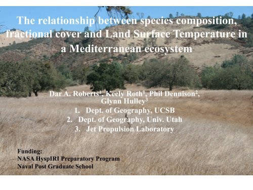
The relationship between species composition,
fractional cover and Land Surface Temperature in
a Mediterranean ecosystem
Dar A. Roberts 1 , Keely Roth 1 , Phil Dennison 2 ,
Glynn Hulley 3
1. Dept. of Geography, UCSB
2. Dept. of Geography, Univ. Utah
3. Jet Propulsion Laboratory
Funding:
NASA HyspIRI Preparatory Program
Naval Post Graduate School

• Introduction
• Research Objectives
• Study Site
• Methods
– Preprocessing
– MESMA
• Results
• Conclusions
Outline

Introduction
• Numerous Synergies exist between the VSWIR and TIR
• VSWIR
– Species composition
– Fractional cover
– Canopy structure (LAI)
0.7
0.6
Anth Water Ligno-­‐cellulose
– Canopy chemistry
0.5
– Photosynthetic function 0.4 Car
• TIR
0.3
Chl
– Temperature
• Stress measure
0.2
AcerLf
Acerlit
• Evapotranspiration 0.1
Betula
– Emissivity
0
Fagus
• Species composition
350 850 1350 1850 2350
• Canopy chemistry
Wavelength (nm)
• HyspIRI will enable those synergies to be fully explored
and utilized
Reflectance

Research Objectives
• Explore synergies between the VSWIR and TIR
using AVIRIS-MASTER pairs
• Research Questions
– What is the relationship between species composition
and land surface temperature (LST)?
– What is the relationship between fractional cover and
LST?

Study Site (1)

Study Site (2)

Methods: Pre-Processing
• AVIRIS: ATCOR Surface Reflectance
– Scene parameters (sensor height, location, time)
– ATCOR parameters
• rural, 940&1130 nm water vapor
• Scan angle from GLT
• Visibility 80km (default), minor adjacency correction
• MASTER
– JPL MASTER TES online tool
– Varied CO 2 , Ozone, Water vapor
• Tuned using emissivity from Lake Lagunita
• Ozone: 0.5, CO 2 : 370 ppm: Water vapor: 0.8 g (cm)
– Temperature (K), Emissivity (5 bands)
• Both: Georectified (7.5m AVIRIS or 15 m. MASTER) to a
spatially degraded DOQQ (2010)
– Resampled nearest neighbor using Delaney Triangulation

Training/Validation Spectra
• Sampled 23 land-cover/species from 307 polygons
• Random training/validation (10 max, or 50%)
• Three pulls, first pull acceptable (Roth et al., 2012)

Multiple Endmember Spectral Mixture
Analysis (MESMA)
Complexity: 3,2,1 RGB Class Composition: NPV-GV-Soil
• Number and types of em varies per pixel
RGB
• Optimum model and complexity level based on RMS
– 2 em =classified map
• Complexity level selected using RMS change threshold
– 0.007

Endmember Selection: Forced Iterative
Endmember Selection
• Traditional: EAR/
MASA/COB
• Automated: Iterative
Endmember Selection
(IES) (Schaaf/Roth)
• Forced IES
– Injects EMC optimal ems
into IES for weak or
missing classes
– Continues until Kappa
does not improve
– Final library can be cut
off at any number
• 101
Kappa Coefficient
0.8
0.7
0.6
0.5
0.4
0.3
0.2
0.1
0
Injection
Cut off
0 50 100 150 200 250 300 350 400
Number of Endmembers
See Roth et al., 2012

• 2em classification
– 101 endmembers
• 67 GV
• 11 GV-NPV (can be either)
• 3 Rock
• 7 Soil
• 13 urban
• GV
– No mixtures, reduced
redundancy
– 25 endmembers
– 1 to 3 per species
• NPV
– 7 endmembers
– 3 Arcasale, 2 brni, 2 magf
Endmember Spectra

• Soil/Rock
– 8 endmembers
– 2 rocks
– 6 soils
• Impervious/urban
– 10 endmembers
– 2 roads
– 3 tile roofs
– 4 composite roofs
– 1 painted roof
Endmember Spectra

Results: Classification
• Model 101: Kappa 0.555, Overall 56%
• Excellent (> 85%: Green): ARCA-SALE, CISP, ERFA, MAGF, PEAM
• Very good(> 60%: Orange): ADFA, BAPI, CEME, QUAG, SOIL, Urban
• Poor (< 30%: Red): CESP, PISA, UMCA

Results: Classification
• The map is better than the validation suggests
• All but a few classes (PISA, UMCA) are generally correct, BAPI is overmapped
• Polygon Accuracy based on most abundant: 84.7%

Class vs Composition: North
• Class
– ARCASALE
– MAGF
– ERFA
– Lesser ADFA, QUDO/QUAG
– Unclassified (bright MAGF, SOILS)
• Composition
– High GV: QUDO/QUAG (in valleys)
– Mixed GV/NPV: ARCASALE/ERFA
– High NPV: MAGF/BRNI?

Class vs Temperature: North
• Class
– ARCASALE
– MAGF
– ERFA
– Lesser ADFA, QUDO/QUAG
– Unclassified (bright MAGF, SOILS)
• Temperature
– Cool: QUDO/QUAG (in valleys)
– Warm ARCASALE/ERFA
– Hot: MAGF, Soils

Class vs Composition: Central
• Class
– ADFA
– QUDO
– QUAG
– CEME, CECU, CESP
– Rock/Soil
– MAGF
• Composition
– High GV: All but MAGF and River channel
– Mixed GV/NPV: ADFA, BAPI (higher NPV-
probably something else)
– High NPV: MAGF
– High Rock/Soil; River channel

Class vs Temperature: Central
• Class
– ADFA
– QUAG, some QUDO
– CEME, CECU, CESP
– Rock/Soil
– MAGF
• Composition
– Cold: North facing slope, dominated by trees
(QUAG)
– Cool: South facing slopes, flat terrain
dominated by shrubs (ADFA, Ceanothus
– Hot: Bare rock on ridges, river channels,
MAGF

Class vs Composition: South
• Class
– MAGF
– BRNI
– EUSP
– PEAM
– CISP
– BAPI
– Urban/Soil
– Minor Marsh
• Composition
– High GV: PEAM, CISP, EUSP
– Mixed NPV-GV: BAPI
– High NPV: MAGF, BRNI
– High soils/Impervious: Urban

Class vs Temperature: South
• Class
– MAGF
– BRNI
– EUSP
– PEAM
– CISP
– BAPI
– Urban/Soil
– Minor Marsh
• Temperature
– Cold: EUSP
– Cool: PEAM, CISP
– Warm: BAPI, BRNI
– Hot: MAGF, Urban

GV Fraction
1
0.8
0.6
0.4
0.2
Temperature Compositional
0
y = -0.0404x + 13.036
R² = 0.589
-0.2
300 305 310
Temperature
315
(K)
320 325 330
Relationships
• GV fraction strongly inversely correlated with temperature for
vegetated targets
• Shade fraction poorly correlated (high shade, cooler, r 2 =0.04)
– Shade is not just shadows, but also varies with albedo and local zenith
Shade Fraction
0.5
0.4
0.3
0.2
0.1
0
-0.1
-0.2
-0.3
300 305 310
Temperature
315
(K)
320 325 330

GV Fraction
1
0.8
0.6
0.4
0.2
0
Temperature Species Relationships
-0.2
300 305 310
Temperature
315 320
(K)
325 330 335
adfa arcasale argl bapi brni
cecu cesp cisp erfa eusp
irgr mafg marsh peam pisa
plra quag qudo umca
• Species composition strongly impacts
temperature, significant clustering
• Trees (circles)
– Coolest, high to moderate GV
• Evergreen shrubs (diamonds)
– Warmer, high to moderate GV
• Deciduous shrubs (triangles)
– Warm, moderate to low GV
• Forbs/grasses (squares)
– High to low GV, warm to hot

Conclusions
• MESMA was capable of mapping 23 species/landcover classes at
reasonable accuracies
– Other classifiers can do better (i.e., LDA/CDA)
• Plant species map out correctly in geographic space
• GV and temperature are inversely correlated
• Plant species cluster uniquely in compositional temperature
space, likely resulting from functional differences
– (e.g., deeply rooted, evapotranspiring cool trees vs shallow rooted
partially senesced shrubs)
• More is coming
– LDA species maps
– EWT – emissivity
– Water vapor TES
– Full range spectroscopy
– And HyspIRI!