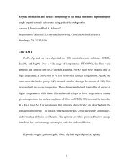
Experimental Method for Determining Surface Energy - Materials ...
Experimental Method for Determining Surface Energy - Materials ...
Experimental Method for Determining Surface Energy - Materials ...

You also want an ePaper? Increase the reach of your titles
YUMPU automatically turns print PDFs into web optimized ePapers that Google loves.
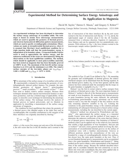
journal<br />
<strong>Experimental</strong> <strong>Method</strong> <strong>for</strong> <strong>Determining</strong> <strong>Surface</strong> <strong>Energy</strong> Anisotropy and<br />
Its Application to Magnesia<br />
David M. Saylor,* Darren E. Mason, † and Gregory S. Rohrer* ,‡<br />
Department of <strong>Materials</strong> Science and Engineering, Carnegie Mellon University, Pittsburgh, Pennsylvania 15213-3890<br />
An experimental technique has been developed to determine<br />
the surface energy anisotropy of crystalline solids. The technique<br />
is based on atomic <strong>for</strong>ce microscopy measurements,<br />
which are used to quantify the geometry of thermal grooves,<br />
and electron backscattered diffraction pattern measurements,<br />
which are used to specify crystallographic orientations. Observations<br />
are made at circumferential thermal grooves, where it<br />
is assumed that Herring’s local equilibrium condition <strong>for</strong> a<br />
triple junction holds and that the grain-boundary energy is<br />
independent of its boundary plane. A truncated double Fourier<br />
series is used to approximate the surface energy, and the<br />
unknown coefficients of the series are determined by fitting the<br />
observations to the local equilibrium condition. The method,<br />
which should be applicable to most polycrystalline materials,<br />
has been tested on magnesia that has been thermally grooved<br />
at 1400°C in air. The maximum of the best-fit surface energy<br />
function is at (111) and the minimum is at (100). The relative<br />
surface energies of the low-index planes are 110 / 100 <br />
1.040 0.008 and 111/ 100 1.072 0.010.<br />
I. Introduction<br />
THE anisotropy of the surface energy of a crystalline solid can be<br />
experimentally evaluated by measuring the geometry of crys-<br />
tallographically indexed surface features. For example, the equilibrium<br />
geometries of thermal facets, 1,2<br />
grain-boundary<br />
grooves, 3–9 small crystallites, 10,11 and internal cavities 12–14 have<br />
been used to deduce relative surface energies. Because these<br />
techniques demand either special microstructural features or specimen<br />
geometries, each has a limited range of applicability. In this<br />
paper, we describe a new technique <strong>for</strong> determining the anisotropy<br />
of the surface energy. The technique involves the analysis of<br />
thermal grooves in typical polycrystals, and we illustrate its<br />
application by describing a measurement of the surface energy<br />
anisotropy of magnesia.<br />
The condition <strong>for</strong> local equilibrium that relates the geometry of<br />
a thermal groove (the dihedral angles at the triple line) and its<br />
crystallography (the crystallite orientations) to the energies of the<br />
three interfaces was originally described by Herring: 15<br />
<br />
i<br />
it i n i<br />
i i 0 (1)<br />
where i is the excess free energy per unit area of the ith interface,<br />
t i the unit vector that lies in the ith interface and is normal to the<br />
C. A. Handwerker—contributing editor<br />
Manuscript No. 189348. Received May 17, 1999; approved October 21, 1999.<br />
Supported primarily by the MRSEC Program of the National Science Foundation<br />
under Award No. DMR-9632556.<br />
*Member, American Ceramic Society.<br />
† Current address: Department of <strong>Materials</strong> Science and Mechanics, Michigan State<br />
University, East Lansing, MI 48864.<br />
‡ Author to whom correspondence should be addressed.<br />
1226<br />
J. Am. Ceram. Soc., 83 [5] 1226–32 (2000)<br />
line of intersection of the three interfaces (l), n i the unit vector<br />
normal to the line of intersection such that n i l tˆ i, and i the<br />
right-handed angle of rotation about l <strong>for</strong> the ith boundary<br />
measured from a reference direction. Equation (1) represents a<br />
<strong>for</strong>ce balance and can be separated into two perpendicular components.<br />
With reference to Fig. 1, the <strong>for</strong>ce balance normal to the<br />
macroscopic sample surface (parallel to e 3)is<br />
3 cos 3 sin 1 cos 1 1 sin 1 1 2 cos 2 2 sin 2 (2)<br />
2 and the <strong>for</strong>ce balance parallel to the macroscopic sample surface is<br />
3 sin 3 cos 1 sin 1 1 cos 1 1 2 sin 2 2 cos 2 (3)<br />
2 The symbols in Eqs. (2) and (3) are defined in Fig. 1. By measuring<br />
the geometry and crystallography of thermal grooves, the relative<br />
interfacial energies can be determined from the Herring equation. In<br />
past thermal groove studies, Eq. (3) has been ignored, and the data<br />
analysis has been conducted under the assumption that the torque on<br />
the grain boundary is negligible (3/ 0). 3–9<br />
Mykura 3 was the first to extract relative surface energies from<br />
an analysis of thermal groove data. The most important feature of<br />
Mykura’s 3 method is that all of the thermal groove measurements<br />
are made at twin boundaries. By measuring only thermal grooves<br />
at grain boundaries having the same character, the potentially<br />
overwhelming grain-boundary energy anisotropy can be eliminated<br />
in such a way that the energies of the free surfaces are the<br />
only remaining unknown variables in Eq. (2). Limiting the<br />
variations in the grain-boundary energy is the common principle<br />
underpinning all subsequent thermal-groove-based surface energy<br />
measurements, including the one described in the current paper.<br />
Mykura’s 3 method was advanced by Winterbottom and Gjostein,<br />
6,7 who approximated the surface energy as a truncated<br />
double Fourier series and used the method of least squares to<br />
determine the unknown coefficients of the series that best fitted a<br />
set of thermal groove observations. One limitation of Mykura’s 3<br />
method is that it can be applied only to the relatively few materials<br />
that exhibit a high population of twin boundaries. McLean and<br />
co-workers 8,9 devised a more general method involving the characterization<br />
of circumferential thermal grooves on the surface of<br />
cylindrical wires with a bamboo microstructure. Grooves at<br />
different positions around the circumference of the wire are<br />
bounded by a range of crystallographically distinct free surfaces,<br />
but always have the same grain boundary at the root. Thus, if<br />
several hundred thermal groove measurements can be accumulated<br />
from a few grain boundaries, Winterbottom and Gjostein’s 6,7 fitting<br />
method can be used to obtain a series representation of the functional<br />
<strong>for</strong>m of the surface energy. Because the methods described above<br />
apply only to crystalline materials that twin extensively or can be<br />
drawn into wires and recrystallized, they have been applied only to<br />
metals such as nickel, 3 copper, 4,8 -iron, 5 and gold. 7
May 2000 <strong>Experimental</strong> <strong>Method</strong> <strong>for</strong> <strong>Determining</strong> <strong>Surface</strong> <strong>Energy</strong> Anisotropy and Its Application to Magnesia 1227<br />
Fig. 1. Coordinate system used <strong>for</strong> the data analysis. (a) Schematic plane<br />
view of an island grain (labeled 2) within a matrix grain (labeled 1).<br />
Multiple groove measurements are made around the circumference of the<br />
island grain, at points labeled P i. (b) Schematic cross-section view of a<br />
triple junction. Note that l points into the plane of the paper.<br />
In the present article, we describe an experimental method that<br />
is similar in spirit to those described above but that can be applied<br />
to ceramic polycrystals. The only necessary property of the<br />
polycrystal is that its microstructure contains a few island grains,<br />
or grains enclosed completely or partially by others. The orientation<br />
dependence of the surface energy of magnesia at 1400°C has<br />
been determined by fitting observations recorded at such grooves<br />
to Herring’s 15 equilibrium condition. The energy function derived<br />
from these data is consistent with observed surface faceting.<br />
II. <strong>Experimental</strong> Procedure<br />
(1) <strong>Experimental</strong> Approach<br />
When examining a well-annealed, polycrystalline microstructure,<br />
a small grain enclosed within a larger grain is occasionally<br />
found. We refer to the smaller, surrounded crystal as an island<br />
grain and the larger crystal as the matrix grain. A planar section<br />
illustrating this situation is shown schematically in Fig. 1(a); an<br />
island grain observed in magnesia is illustrated in Fig. 2. In Fig. 2,<br />
the boundary separating the island grain from the matrix grain is<br />
easily distinguished by the thermal groove. Assuming that the<br />
triple junction at the groove root is in local thermodynamic<br />
equilibrium, Eqs. (2) and (3) should then be satisfied at all points,<br />
P i. If the orientations of both grains are determined by backscattered<br />
electron diffraction and the inclinations of the three interfaces<br />
(defined by 1, 2, and ) are determined by microscopic<br />
analysis at N points along the boundary, then it is possible to<br />
specify all of the quantities in Eqs. (2) and (3), except the interface<br />
energies and their derivatives. In our analysis, we assume that the<br />
vectors defining the interface tangents and normals lie in a single<br />
planar section that is perpendicular to the tangent of the triple line.<br />
<strong>Determining</strong> the surface energy from the N vector equations is<br />
a highly nonlinear problem that, because of experimental uncertainties,<br />
may not have a classical solution. To determine an<br />
approximate <strong>for</strong>m <strong>for</strong> the surface energy, we make two simplifying<br />
assumptions that allow us to arrive at an overdetermined system of<br />
linear equations. An approximate solution of these equations then<br />
can be found via the method of least squares. First, we assume that<br />
the grain-boundary energy is a function only of the misorientation<br />
and not the boundary plane. There<strong>for</strong>e, 3/ 0; this is identical<br />
to the approximation applied in the earlier work. 3,9 Because the<br />
misorientation is fixed at all points across the boundary, the<br />
grain-boundary energy ( 3) is the same in each of the N equations.<br />
Second, we use Winterbottom and Gjostein’s 6,7 method of approximating<br />
the surface energy as a truncated double Fourier series. We<br />
have selected the following <strong>for</strong>m <strong>for</strong> the function:<br />
R<br />
s, 1 <br />
i1<br />
R<br />
aij cos2i 1 cos j<br />
j0<br />
bij sin2i cos j<br />
cijcos2i 1 sin j<br />
dij sin2i sin j} (4)<br />
In Eq. (4), and are the usual spherical angles, and the energy<br />
of the (100) orientation ( 0) is normalized to equal 1.0. Using<br />
this approximation, the surface energy and its derivatives at each<br />
point are determined by the surface orientation and a finite set of<br />
unknown coefficients. For a series of order R, the number of<br />
coefficients is 2R(2R 1), so that, <strong>for</strong> a set of N observations<br />
Fig. 2. Montage of AFM images showing an island grain. Black-to-white vertical contrast is 200 nm. Contrast discontinuities occur at the points where<br />
images have been pieced together. <strong>Surface</strong>s are inclined from the 111 axis by 10° and are slightly misoriented with respect to one another.
1228 Journal of the American Ceramic Society—Saylor et al. Vol. 83, No. 5<br />
along the circumferences of G island grains, the total number of<br />
unknowns is U 2R(2R 1) G. Because 50 observations<br />
can be made at each island grain, an increment in G increases N much<br />
more than U. Thus, <strong>for</strong> even a few island grains, N U, and a set<br />
of best-fitted coefficients and grain-boundary energies can be determined<br />
using a conventional linear least-squares procedure.<br />
The procedure described above should be widely applicable to<br />
most polycrystalline materials. It is not required that the island<br />
grains be completely isolated in the matrix grain, only that the<br />
observations be accumulated from a boundary with constant misorientation<br />
and a significant degree of curvature (so that surfaces with<br />
many distinct orientations are exposed at the groove root). In our<br />
experience, large curvature is typically observed at low-angle grain<br />
boundaries. In fact, all of the island grains identified as part of this<br />
study have misorientations of 7° and presumably have been <strong>for</strong>med<br />
when a higher-mobility grain boundary has swept past during the<br />
coarsening of the microstructure.<br />
(2) Sample Preparation<br />
Magnesia powder was <strong>for</strong>med by decomposing 99.7%-pure<br />
magnesium carbonate (Fisher Scientific Co., Pittsburgh, PA) at<br />
997°C in air. Uniaxial compaction in a hot press at 1700°C <strong>for</strong> 1 h<br />
at 61 MPa produced a disk with a diameter of 50 mm and an<br />
average thickness of 1.5 mm. Specimens cut from this disk then<br />
were packed in a magnesia crucible with the parent powder and<br />
annealed <strong>for</strong> 48 h at 1600°C in air. At the end of this treatment, the<br />
specimens were translucent. The geometric measurements used to<br />
characterize the thermal groove and grain-boundary geometry<br />
required specimens that are flat and have two parallel faces.<br />
Appropriate surfaces were prepared using an automatic polisher<br />
(Model PM5, Logitech, Inc., Fremont, CA). The surfaces were<br />
initially lapped with a 9 m alumina slurry, and the final polish<br />
was achieved using an alkaline (pH 10) colloidal silica (0.05<br />
m) slurry. The flatness of the final surface was measured using an<br />
inductive axial movement gauge head with a resolution of 0.1 m<br />
(TESR, Model TT22, Brown and Sharpe, Wixom, MI); surfaces<br />
were determined to be flat, within 0.3 m over lateral dimensions<br />
of 1 cm. The surface was thermally grooved by annealing it<br />
inair<strong>for</strong>5hat1400°C. One of the assumptions that underpinned<br />
our measurement was that the groove morphology was determined<br />
at 1400°C and that it did not change in a significant way during<br />
cooling. Considering the fact that the lateral and vertical dimensions<br />
of the grooves and surface facets scaled with the annealing<br />
time and maintain constant dihedral angles, this appeared to be a<br />
satisfactory approximation. The average grain size of the sample<br />
was 109 m. At this stage, one sample was analyzed <strong>for</strong> impurities.<br />
The sample contained 0.2% calcium, 0.02% aluminum, 0.03%<br />
iron, 0.02% silicon, and 0.03% yttrium.<br />
After thermal grooving, many island grains were located, and<br />
optical micrographs were recorded. A thin, uni<strong>for</strong>m layer (in a<br />
typical experiment, 6 0.3 m) then was removed by polishing,<br />
and the thermal groove treatment was repeated. The island grains<br />
that remained after polishing (some terminate in the removed<br />
layer) were characterized more completely, as described below.<br />
(3) Crystallite Orientations<br />
The orientations of the matrix and island grains were determined<br />
from electron backscattered diffraction patterns (EBSPs).<br />
The grooved samples were imaged (uncoated) using scanning<br />
electron microscopy (SEM; Model XL40, Philips, Eindhoven, The<br />
Netherlands). EBSPs were obtained at a specimen tilt of 70° by<br />
pointing the beam at the grain of interest in the spot mode. Patterns<br />
were indexed using ORIENTATION IMAGING MICROSCOPY software,<br />
version 2.6 (TexSEM Laboratories, Inc., Draper, UT), which<br />
returned a set of Euler rotation angles ( 1, , 2) relating the<br />
crystal reference frame to the sample reference frame. The absolute<br />
orientation of each grain was determined from three separate<br />
diffraction patterns recorded in the same grain.<br />
(4) <strong>Surface</strong> Inclinations<br />
The orientations of the free surfaces at the groove root were<br />
determined by combining topographic atomic <strong>for</strong>ce microscopy<br />
(AFM) data with the orientation data derived from the EBSPs. The<br />
AFM data were recorded using a stand-alone AFM (Model<br />
SAA-125, Digital Instruments, Santa Barbara, CA) positioned<br />
above the specimen mounted on an X–Y translation stage (Model<br />
TSE-150, Burleigh Instruments, Fishers, NY) capable of reproducibly<br />
positioning the specimen with 50 nm resolution. Silicon<br />
nitride cantilevers (Model LNP, Digital Instruments) were used as<br />
probes. AFM data were used to determine the partial dihedral<br />
angles ( 1 and 2) and the angle between e 1 and v (see Fig. 1).<br />
The method <strong>for</strong> determining the partial dihedral angles has been<br />
described in detail in a previous paper. 16 Briefly, the width and<br />
depth of the groove are determined from AFM topographs. In<br />
general, the grooves are not symmetric; there<strong>for</strong>e, the groove<br />
width associated with a particular crystallite is assumed to be twice<br />
the distance from the topographic minimum at the groove root to<br />
the crest of the adjacent peak. The depth is the vertical distance<br />
from the minimum at the groove root to the crest of the adjacent<br />
peak. If we assume a quasi-static groove profile, it is possible to<br />
determine the inclination of the surface at the groove root from a<br />
measurement of the width and depth. 16 We have used the relationship<br />
between the width, depth, and inclination determined by<br />
Robertson. 17 Because the analytical <strong>for</strong>m of the quasi-static groove<br />
profile is determined under the assumption that the surface<br />
energies are isotropic, there is an approximation implicit in this<br />
procedure. Based on earlier work, the systematic errors associated<br />
with the tip convolution effect <strong>for</strong> these relatively wide and<br />
shallow grooves should be negligible, and the standard deviation<br />
from random errors is estimated to be 1°. 18<br />
More-significant errors potentially resulted from sample positioning.<br />
Because the surface orientations were determined by<br />
combining AFM and SEM observations, it was important that the<br />
specimen reference frame be coincident with the reference frame<br />
of both microscopes. To assist with alignment, two of the lateral<br />
edges of the specimen were cut so that they <strong>for</strong>med a right angle with<br />
each other and the analysis surface. On each microscope stage, these<br />
external features were used to align the specimen. We estimated that<br />
the uncertainty in the orientation that results from indexing and<br />
specimen positioning errors was not greater than 5°.<br />
Based on the AFM data, the normal of the surface at the groove<br />
root (n i) has the following components in the laboratory reference<br />
frame:<br />
n i,1 cos i cos <br />
n i,2 cos i sin <br />
n i,3 1 i sin i<br />
where the subscript i refers to the surfaces labeled in Fig. 1. The<br />
normal vector n 1 is defined as pointing into the crystal. In the<br />
crystal reference frame, the components of the surface normal (z i)<br />
are specified according to the following trans<strong>for</strong>mation:<br />
z i g ijn j<br />
where g ij is given by 19<br />
g1 ,, 2 <br />
c1c2 s1s2c s1c2 c1s2c s2s c1s2 s1c2c s1s2 c1c2c c2s <br />
s1s c1s c<br />
where c and s represent sine and cosine, respectively. Finally, the<br />
surface normals are trans<strong>for</strong>med to a unit triangle of distinct<br />
orientations in cubic orientation space where the normal vector n<br />
has the components z i:<br />
z i M ikz k<br />
(5)<br />
(6)<br />
(7)<br />
(8)
May 2000 <strong>Experimental</strong> <strong>Method</strong> <strong>for</strong> <strong>Determining</strong> <strong>Surface</strong> <strong>Energy</strong> Anisotropy and Its Application to Magnesia 1229<br />
The components of n are permutations of the absolute values of zi, such that z 1 z 2 z 3, and the values of Mik are 0, 1, or 1 and<br />
are assigned in the following way. If z i zk, then Mik 0. If z i <br />
zk, then Mik 1 <strong>for</strong> positive zk, and Mik 1<strong>for</strong> negative zk. The<br />
surface energy is parameterized in terms of the spherical coordinates<br />
and ; the relationship between these variables and the<br />
components of the surface normal are<br />
cos1 z1 (9)<br />
tan1 z3 z2 The torque terms in Eqs. (2) and (3) can be evaluated using the<br />
following expression:<br />
i i <br />
i<br />
i i <br />
i <br />
(10)<br />
Analytical expressions <strong>for</strong> i/ and i/ are easily obtained<br />
from Eq. (4). Although the terms / i and / i can be derived<br />
exactly, <strong>for</strong> computational ease they have been approximated as<br />
difference quotients, / i and / i, calculated by dividing<br />
the change that occurs in or ( or ) as the surface normal<br />
vector is rotated through a small, fixed angle about l, by the<br />
rotation angle ( i). The values of and have been<br />
determined using a rotation matrix with elements R ij:<br />
R ij ij cos ε ijkl k sin 1 cosl il j<br />
(11)<br />
where l i are the components of the vector l, ij the Kronecker delta,<br />
and ijk the permutation tensor. The results of the fit are insensitive<br />
to choices of 1°.<br />
(5) Boundary Inclinations<br />
Optical micrographs of each island grain were recorded be<strong>for</strong>e<br />
and after a thin layer of the specimen was removed by polishing.<br />
The field of view <strong>for</strong> these micrographs included approximately 20<br />
additional grains in the adjacent microstructure so that the relative<br />
lateral positions of the two images could be determined by visually<br />
maximizing the overlap of all the grain boundaries in the image.<br />
Based on measurements of the amount of material removed and<br />
the apparent lateral shift of the boundary between the two images,<br />
the inclination () at each point (P i) was determined. Considering<br />
the magnitude of the vertical distance (6 0.3 m) and our<br />
estimated uncertainty in the lateral registry between the two layers<br />
(1.5 m), we anticipated that the maximum uncertainty on was<br />
14°. This was by far the most uncertain measurement in this<br />
experiment, and the impact of this error is described in the<br />
Discussion section.<br />
(6) Fitting<br />
The approximate expression <strong>for</strong> the surface energy (Eq. (4)) was<br />
substituted into Eqs. (2) and (3), and a standard linear least-squares<br />
procedure (LSFIT 20 ) was used to determine the best-fitted values<br />
of the coefficients. The quality of the fit was assessed by the ratio<br />
() of the sum of the squares of the residuals to the difference<br />
between the number of equations and the number of free parameters.<br />
The results presented in the next section are based on fits to<br />
Eq. (2). Fits that included Eqs. (2) and (3) yielded qualitatively<br />
similar results, but the value of was 5 times larger. Possible<br />
reasons <strong>for</strong> this are described in the Discussion section. The data<br />
set consisted of 269 observations from five island grains. If a series<br />
of order R 1 is used, then 6.76 10 3 . When the data set<br />
was randomly partitioned into two smaller segments, fitting to<br />
each segment led to almost identical results (within the standard<br />
deviation of the fit). When more terms were included in the series,<br />
there were additional oscillations in the function, and decreased<br />
slightly. For example, when R 2, 5.47 10 3 . In this case,<br />
the ordering of the relative energies at the low index surfaces was<br />
the same as <strong>for</strong> the R 1 fit. However, when the R 2 function<br />
was fitted to the randomly partitioned data sets, the results differed<br />
from one another and from the results obtained using the complete<br />
data set. For this reason, we took the result from the R 1 series<br />
to be the more reliable result.<br />
(7) Orientation Stability<br />
AFM images of the specimen revealed that the surfaces of some<br />
grains were faceted (<strong>for</strong> example, see Fig. 2), whereas others were<br />
smooth. The faceted surfaces always contained ridges <strong>for</strong>med by<br />
the intersection of two planes, but no corners. When the surface<br />
inclination changed, as it did near a thermal groove, the ridges<br />
exhibited smoothly curved edges. Thus, all missing surface orientations<br />
could be made up of two stable planes. To map the<br />
orientations that were stable or unstable with respect to faceting,<br />
AFM images were recorded of the surfaces of more than 100<br />
grains whose orientations were previously determined based on<br />
EBSP data. If steps with heights 2.1 nm were observed (this<br />
corresponds to 5 times the lattice spacing), the grain was labeled as<br />
faceted. If no steps or steps less than this height were observed, the<br />
grain was labeled as smooth. We choose this arbitrary cutoff as a<br />
dividing line between discrete and continuum behavior by assuming<br />
that, <strong>for</strong> steps of this height, the interaction between individual<br />
atoms at the top and bottom of the facet was negligible.<br />
III. Results<br />
The best-fitted coefficients <strong>for</strong> the series in Eq. (4) are listed in<br />
Table I. Based on these values, we calculated the energies of the<br />
low-index planes to have the following relations:<br />
110 100 111 100 1.040 0.008<br />
1.072 0.010<br />
The uncertainties in the values of the energy were determined from<br />
the variances and covariances of the fitted coefficients. 21 The<br />
maximum energy occurred at the (111) orientation and the minimum<br />
at (100). The functional dependence is illustrated in Fig. 3,<br />
where the value of the function at each observed orientation (Fig.<br />
3(a)) and the energy contours (Fig. 3(b)) are plotted in a unit<br />
triangle of distinguishable orientations. The value of the surface<br />
energy function along the perimeter of the unit triangle is graphed<br />
in Fig. 4. The best-fitted grain-boundary energies <strong>for</strong> each of the<br />
island grains are listed in Table II. In each case, the energy is less<br />
than that of the (100) surface.<br />
The orientation stability map is shown in Fig. 5. With the<br />
exception of two outliers and a small amount of overlap in the<br />
distributions, the faceted and smooth orientations are well separated.<br />
Based on these data, it seems that surface orientations near<br />
(100) and (111) are unstable with respect to faceting.<br />
IV. Discussion<br />
Ignoring relaxation effects, the relative surface energy of<br />
different crystallographic planes should scale with the broken bond<br />
Table I. Best Fitted<br />
Coefficients <strong>for</strong> the<br />
<strong>Surface</strong> <strong>Energy</strong> Function<br />
Coefficient Value †<br />
a10 b10 a11 b11 c11 d11 0.118 (60)<br />
0.084 (36)<br />
0.130 (60)<br />
0.056 (34)<br />
0.100 (22)<br />
0.438 (12)<br />
† Standard deviation in the last<br />
two digits is given in parentheses.
1230 Journal of the American Ceramic Society—Saylor et al. Vol. 83, No. 5<br />
Fig. 3. (a) Orientations of surfaces at the groove roots of five island<br />
grains, plotted in a unit triangle of distinguishable orientations. Each point<br />
is shaded to represent the value of the best-fitted function at that point,<br />
where black corresponds to hkl 1.000 and white corresponds to hkl <br />
1.072. (b) <strong>Surface</strong> energy contour plot constructed from the fitted function.<br />
Shading of the contours is the same as in (a).<br />
Fig. 4. Plot of the relative surface energy around the perimeter of the unit<br />
triangle, from (100) to (111), then to (110), and back to (100).<br />
Table II. Best-Fitted Grain-Boundary Energies<br />
<strong>Energy</strong> Relative<br />
to 100 †<br />
Misorientation<br />
(deg) Axis<br />
0.80 (1) 6.25 0.99 0.13 0.06<br />
0.90 (1) 2.33 0.79 0.61 0.04<br />
0.55 (2) 3.14 0.69 0.68 0.28<br />
0.52 (2) 2.02 0.81 0.58 0.02<br />
0.87 (2) 6.31 0.92 0.33 0.20<br />
† Standard deviation in the last digit is given in parentheses.<br />
density. Magnesia has the rock salt structure and only one bond per<br />
atom must be broken to create the (100) surface. Two and three<br />
bonds per atom must be broken to <strong>for</strong>m the (110) and (111)<br />
surfaces, respectively. When the broken bond densities per unit<br />
area () are compared, the (100) surface has the smallest value and<br />
110 / 100 2 1/2 and 111/ 100 3 1/2 . There<strong>for</strong>e, the measured<br />
surface energies occur in the same order as the density of<br />
nearest-neighbor broken bonds on the surface. As expected,<br />
however, the measured variation in the energies in the real system<br />
(7%) is much less than that predicted by the simple bond-breaking<br />
Fig. 5. Orientation stability map <strong>for</strong> magnesia at 1400°C. Each point<br />
corresponds to the orientation of an observed grain. Grains that are faceted<br />
are marked with an , and grains that are smooth are marked with an open<br />
square.<br />
model. Anisotropies of 2%–8% have been previously observed in<br />
face-centered cubic (fcc) metals; 3–11 the current observations are<br />
consistent with the higher end of this range and less than the<br />
anisotropy reported <strong>for</strong> lithium fluoride (18%) 13 and sapphire<br />
(12%). 14<br />
The only previous experimental evaluation of the surface<br />
energy of magnesia was reported by Jura and Garland; 22 their<br />
calorimetric study of a fine powder led to the conclusion that the<br />
average surface energy of magnesia at room temperature is 1.0<br />
J/m 2 . Because the adsorption of water probably influenced this<br />
experiment, this value is likely to be an underestimate. There also<br />
have been model calculations of the surface energy of magnesia,<br />
and they are summarized in Table III. 23–27 With one exception,<br />
these studies place the energy of the (100) surface at 1.0 J/m 2 at<br />
0 K. Furthermore, in the cases where the energies of more than one<br />
surface have been computed, the energies have the same order as<br />
those observed in the present study ( 100 110 111). The<br />
magnitude of the anisotropy predicted by these 0 K calculations is<br />
larger than experimentally observed and, in fact, is larger than it<br />
would be possible to observe in any equilibrium experiment. For<br />
example, if the energy of the (110) surface of a cubic crystal were<br />
2 1/2 times the energy of the (100) surface, then the surface would<br />
lower its energy by faceting into (100) and (010) surfaces that<br />
would meet along lines in the [001] direction and <strong>for</strong>m ridges.<br />
There<strong>for</strong>e, the energy of the (110) orientation has an upper limit of<br />
2 1/2 100. Similarly, if the energy of the (111) surface were 3 1/2<br />
times the energy of the (100) surface, it would lower its energy by<br />
faceting into trigonal pyramids bound by (100), (010), and (001)<br />
facets. Thus, the results of our experiments fall within the upper<br />
bounds set by the equilibrium condition.<br />
A Wulff <strong>for</strong>m was constructed based on the best-fitted energy<br />
function, and it is shown in Fig. 6. To construct the shape,<br />
orientation space was discretized (steps of 0.05 in k and l), and the<br />
surface energy of each orientation was assigned based on the<br />
best-fitted function. By applying the Wulff construction, a point on<br />
Table III. Model Calculations of the Magnesia <strong>Surface</strong><br />
<strong>Energy</strong><br />
<strong>Surface</strong> energy (J/m2 )<br />
(100) (110) (211) (111)<br />
<strong>Method</strong> †<br />
1.16 2.92 Electrostatic model 21<br />
1.43 Ab initio Hartree–Fock LCAO 22<br />
1.07 2.78 Electrostatic model 23<br />
2.64 12.80 Harris–Foulkes functional (LDA) 24<br />
0.98 2.29 4.35 Self-consistent tight binding 25<br />
† LCAO is linear combination of atomic orbitals and LDA means local density<br />
approximation.
May 2000 <strong>Experimental</strong> <strong>Method</strong> <strong>for</strong> <strong>Determining</strong> <strong>Surface</strong> <strong>Energy</strong> Anisotropy and Its Application to Magnesia 1231<br />
Fig. 6. Wulff shape of magnesia at 1400°C, determined from the fitted<br />
surface energy function.<br />
the surface of the Wulff shape was found <strong>for</strong> each orientation. The<br />
space between each point then was filled in by QHULL and rendered<br />
in GEOMVIEW to create Fig. 6. 28<br />
Because of the discretization, continuously curved surfaces<br />
appear as regular arrays of flat squares visible in the detail of Fig.<br />
6. There are, however, two other features that derive from the<br />
shape of the surface energy function. The first feature is the small<br />
flat facet at (100). Based on the extent of this facet, we conclude<br />
that {hk0} orientations inclined by 5.7° from (100) are missing<br />
from the Wulff <strong>for</strong>m. The second feature is the sharp edges <strong>for</strong>med<br />
by the intersections of the curved surfaces. These edges pass<br />
through (110) and meet at the (111) orientation. This means that<br />
orientations in the vicinity of the (111) orientation are missing and<br />
that the range of missing orientations extends toward the (110)<br />
orientation. It must be noted that the details of the Wulff <strong>for</strong>m are<br />
extremely sensitive to the details of the energy function, which<br />
contains some uncertainty and is constrained by the choice of basis<br />
functions. 9 Increasing or decreasing the energies of selected<br />
orientations within the uncertainties of the function can affect the<br />
extent of the missing orientations in a significant way. However,<br />
we can test the validity of the Wulff <strong>for</strong>m in Fig. 6 by comparing<br />
it with the orientation stability data.<br />
The orientation stability figure presented in Fig. 5 indicates that<br />
surfaces inclined from (100) by 5° are unstable with respect to<br />
faceting. This result is consistent with the Wulff shape illustrated<br />
in Fig. 6, which shows that these orientations are missing from the<br />
equilibrium <strong>for</strong>m. Orientations in the missing region break up into<br />
a (100) facet and a complex (high-index) facet 5° from (100).<br />
The specific index of the complex facet depends on the grain<br />
orientation. The angle at which the (100) plane intersects the<br />
complex surface can be used as an independent measure of the<br />
relative energy of the (100) plane ( 100) and the complex plane<br />
( c). When the Herring equilibrium condition is applied to the<br />
intersection of these two facets, we find that 2,15<br />
100 cos <br />
c 1 c sin (12)<br />
c <br />
Taking the second term in Eq. (12) to be negligible (<strong>for</strong> small ,<br />
where is the angle between the surface normals), the relative<br />
energy is given by cos , which indicates that c/100 1.004.<br />
This is consistent with the best-fitted surface energy function (see<br />
Fig. 4).<br />
The faceted area near the (111) pole spans a much larger<br />
angular range than that near (100). Considering that the surface<br />
energy function maximizes at this orientation, we conclude that<br />
surfaces with these orientations facet to neighboring complex<br />
planes. The observation of faceting in this area is consistent with<br />
the Wulff shape, which shows curved surfaces meeting at sharp<br />
edges that intersect at {111} poles. The sharp edges on the Wulff<br />
shape occur when there are missing orientations; grains with such<br />
orientations may facet. The range of faceted orientations indicated<br />
in Fig. 5 appears to be larger than the range of missing orientations<br />
shown in Fig. 6. The observations also can be explained if the<br />
(111) orientation actually has a slightly lower energy than the<br />
surrounding orientations. In other words, within the uncertainty of<br />
the best-fitted function, it is possible that the surface energy<br />
maximum is inclined a few degrees from (111) and that the (111)<br />
orientation is a local minimum. If this were the case, then the<br />
orientations in the unstable region would always break up into a<br />
facet near (111) and a complex plane at the boundary between the<br />
smooth and faceted orientations. In principle, it should be possible<br />
to distinguish between these two scenarios by indexing the facets<br />
based on EBSP and AFM data. In this particular case, however, the<br />
small spacing of the facets makes their inclinations difficult to<br />
accurately quantify, and our measurements to date have led to<br />
ambiguous results. Although the ambiguous results most likely<br />
occur because of difficulties associated with the measurement, it is<br />
also possible that the shape of the energy function is more<br />
complicated than either of the two scenarios presented above.<br />
The shape of the energy function that results from our fitting<br />
procedure is ultimately constrained by the number of harmonics<br />
used to approximate the energy. If complicated variations do<br />
occur, they are not reproduced by our function. However, the<br />
conclusion that the surface energy increases as the (111) orientation<br />
is approached is robust and consistent with theoretical<br />
predictions and earlier observations. The (111) surface of a<br />
compound with the rock salt structure is polar (terminated by ions<br />
with the same charge), and it has been argued that, because a polar<br />
surface has a dipole moment, its energy is always larger than the<br />
energies of other surfaces of the same solid that are either charge<br />
neutral or charged, but lacking a dipole moment. 29 The conventional<br />
view is that orientations vicinal to a low-index plane have<br />
relatively higher energies, because additional bonds must be<br />
broken to create a terrace–step structure. However, this rational<br />
does not necessarily apply to a polar surface. In this case, although<br />
the step creation does break additional bonds, it also introduces<br />
ions of the opposite sign, and this reduces the surface charge<br />
imbalance. For example, adjacent (111) terraces of the rock salt<br />
structure separated by monoatomic steps are terminated by ions of<br />
opposite charge. Thus, a decrease in the surface energy with step<br />
density can occur if the gain in electrostatic stability is greater than<br />
the cost of breaking bonds to create steps.<br />
Earlier experimental studies of magnesia surfaces have been<br />
conducted in temperature ranges above and below the current<br />
study (but at different partial pressures of oxygen). For example,<br />
Henrich 30 annealed an ion-bombarded magnesia (111) surface<br />
under ultrahigh vacuum to temperatures as high as 1127°C and<br />
found that the surface faceted into trigonal pyramids bounded by<br />
(100) planes. This would imply a higher degree of anisotropy than<br />
what we have observed, which would be consistent with the lower<br />
temperatures used <strong>for</strong> the annealing. When the magnesia (111)<br />
surface was examined by reflection electron microscopy after<br />
being annealed at 1550°–1700°C in oxygen, it was found to be<br />
smooth (but reconstructed on the atomic scale) and stable against<br />
faceting. 31 Although the widely different partial pressures of<br />
oxygen used in the a<strong>for</strong>ementioned studies might make a rigorous<br />
comparison inappropriate, the transition from a faceted surface at<br />
1127°C 30 to a partially faceted surface at 1400°C (the current<br />
study) and to a smooth surface at 1500°C 31 is consistent with the<br />
reduction in anisotropy that is expected at elevated temperatures.<br />
In fact, this transition might be analogous to that observed in the<br />
isostructural compound halite, <strong>for</strong> which smooth (111) surfaces are<br />
observed only above 650°C. 32 In the present and previous studies,<br />
calcium was the major impurity, and this is known to segregate to<br />
the surface. 33 Reflection electron microscopy experiments have<br />
shown that the step structure on the (100) surface can be altered by<br />
calcium segregation; 34 there<strong>for</strong>e, we must conclude that the exact<br />
<strong>for</strong>m of the surface energy function is sensitive to the temperature<br />
and partial pressure of oxygen, and to the concentration of<br />
dissolved (and segregated) impurities.
1232 Journal of the American Ceramic Society—Saylor et al. Vol. 83, No. 5<br />
The best-fitted grain-boundary energies (see Table II) are all<br />
less than the surface energy. The median grain boundary to surface<br />
energy ratio has been previously measured to be 1.2, which<br />
indicates that most of the grain boundaries in a random polycrystal<br />
have an energy that is greater than the surface energy. 16,35 The<br />
distribution of energy ratios, however, extends as low as 0.65 <strong>for</strong><br />
low-angle boundaries. 16 There<strong>for</strong>e, the low energies that result<br />
from our fit are not surprising, considering that the largest<br />
misorientation is 7°. With one exception, the fitted grainboundary<br />
energy increases with the misorientation angle. Although<br />
the exception might be due to experimental error, it is probably not<br />
appropriate to establish a correlation between the grain-boundary<br />
energy and only one of the five macroscopic degrees of freedom<br />
that define the grain-boundary character.<br />
One of the assumptions applied in our analysis is that the<br />
grain-boundary energy is independent of the boundary plane. In<br />
other words, the energy of the grain boundary at all points around<br />
the thermal groove is assumed to be the same. If the best-fitted<br />
surface energy function is used to determine the energies of the<br />
surfaces bounding the groove at each point around an island<br />
grain’s circumference, the Herring 15 equilibrium condition can be<br />
used to compute a boundary energy at each point. Energies<br />
computed in this way vary systematically with position and<br />
suggest that the boundary plane does influence the grain-boundary<br />
energy. That we average over these variations in our fitting<br />
procedure (and ignore the grain-boundary torque terms) is one of<br />
the sources of uncertainty in our result.<br />
Finally, Eq. (3) has been neglected in our fitting procedure. In<br />
earlier work, Eq. (3) has been ignored without comment. 3–9<br />
Including Eq. (3) in the procedure described here increases the<br />
uncertainty in the result. The reason <strong>for</strong> this is evident when we<br />
compare the <strong>for</strong>m of the equations. In Eqs. (2) and (3), the<br />
magnitude of the left-hand side is determined by , a measured<br />
parameter that is typically near zero (78% of the observations are in<br />
the range 20° 20°) and contains the highest degree of<br />
experimental uncertainty. The left-hand side of Eq. (2) scales with cos<br />
, and the left-hand side of Eq. (3) scales with sin , so that, when <br />
is small, measurement errors are magnified by Eq. (3) and diminished<br />
by Eq. (2). For example, a 15° error in the measurement of 0<br />
leads to an uncertainty on the left-hand side of Eq. (2) of 3.5%; <strong>for</strong> Eq.<br />
(3), the same error leads to an uncertainty of 26%.<br />
An alternate approach to reconstructing the surface energy<br />
function from thermal groove data, which considers both components<br />
of Eq. (1), is described in the <strong>for</strong>thcoming paper. 36 This new<br />
method is statistical in nature, multiscale in implementation, and<br />
af<strong>for</strong>ds efficient incorporation of the full vector equilibrium<br />
equation. Other main advantages in this approach include no a<br />
priori basis selection <strong>for</strong> the surface energy representation and<br />
efficient accommodation of large amounts of experimental data.<br />
V. Conclusions<br />
An experimental technique has been developed to determine the<br />
anisotropy of surface energy. The technique uses polycrystalline<br />
specimens and is based on the analysis of crystallographic data<br />
obtained from EBSPs and geometric data obtained by AFM. We<br />
have tested the method on magnesia and found that, at 1400°C,<br />
110 / 100 1.040 0.008 and 111/ 100 1.072 0.010. The<br />
surface energy minimum is at (100), and this leads to the faceting<br />
of orientations within 5° of this surface. The surface energy<br />
maximum occurs at or very near the (111) orientation, which is a<br />
polar surface. An orientation stability map indicates that orientations<br />
near (111) are unstable with respect to faceting. It should be<br />
possible to conduct similar measurements on any polycrystalline<br />
specimen that has a grain size 30 m and contains some<br />
enclosed or partially enclosed grains.<br />
References<br />
1 A. J. W. Moore, “The Influence of <strong>Surface</strong> <strong>Energy</strong> on Thermal Etching,” Acta<br />
Metall., 6 [4] 293–304 (1958).<br />
2 A. J. W. Moore, “Thermal Faceting”; pp. 155–98 in Metal <strong>Surface</strong>s: Structure,<br />
Energetics, and Kinetics. Edited by N. A. Gjostein and W. D. Robertson. American<br />
Society <strong>for</strong> Metals, Metals Park, OH, 1963.<br />
3 H. Mykura, “The Variation of the <strong>Surface</strong> Tension of Nickel with Crystallographic<br />
Orientation,” Acta Metall., 9 [6] 570–76 (1961).<br />
4 W. M. Robertson and P. G. Shewmon, “Variation of the <strong>Surface</strong> Tension with<br />
Orientation in Copper,” Trans. Metall. Soc. AIME, 224 [4] 804–11 (1962).<br />
5 M. McLean and H. Mykura, “The Orientation Dependence of <strong>Surface</strong> Tension <strong>for</strong><br />
Face-Centered-Cubic Iron,” Acta Metall., 12 [3] 326–28 (1964).<br />
6 W. A. Winterbottom and N. A. Gjostein, “Determination of the Anisotropy of<br />
<strong>Surface</strong> <strong>Energy</strong> of Metals—I: Theoretical Analysis,” Acta Metall., 14 [9] 1033–40<br />
(1966).<br />
7 W. A. Winterbottom and N. A. Gjostein, “Determination of the Anisotropy of<br />
<strong>Surface</strong> <strong>Energy</strong> of Metals—II: <strong>Experimental</strong> -Plot of Au,” Acta Metall., 14 [9]<br />
1041–52 (1966).<br />
8 M. McLean and B. Gale, “<strong>Surface</strong> <strong>Energy</strong> Anisotropy by an Improved Thermal<br />
Grooving Technique,” Philos. Mag., 20 [167] 1033–45 (1969).<br />
9 B. Gale, R. A. Hunt, and M. McLean, “An Analysis of <strong>Surface</strong> <strong>Energy</strong> Anisotropy<br />
Data Using Lattice Harmonics,” Philos. Mag., 25 [4] 947–60 (1972).<br />
10 J. C. Heyraud and J. J. Métois, “Equilibrium Shape and Temperature; Lead on<br />
Graphite,” Surf. Sci., 128 [2/3] 334–42 (1983).<br />
11 J. C. Heyraud and J. J. Métois, “Equilibrium Shape of Gold Crystallites on a<br />
Graphite Cleavage <strong>Surface</strong>: <strong>Surface</strong> Energies and Interfacial <strong>Energy</strong>,” Acta Metall.,<br />
28 [12] 1789–97 (1980).<br />
12 R. S. Nelson, D. J. Mazey, and R. S. Barnes, “The Thermal Equilibrium Shape<br />
and Sizes of Holes in Solids,” Philos. Mag., 11 [109] 91–111 (1965).<br />
13 Z. Y. Wang, M. P. Harmer, and Y. T. Chou, “Pore–Grain Boundary Configurations<br />
in Lithium Fluoride,” J. Am. Ceram. Soc., 69 [10] 735–40 (1986).<br />
14 J.-H. Choi, D.-Y. Kim, B. J. Hockey, S. M. Wiederhorn, C. A. Handwerker, J. E.<br />
Blendell, W. C. Carter, and A. R. Roosen, “Equilibrium Shape of Internal Cavities in<br />
Sapphire,” J. Am. Ceram. Soc., 80 [1] 62–68 (1997).<br />
15 C. Herring, “<strong>Surface</strong> Tension as a Motivation <strong>for</strong> Sintering”; pp. 143–79 in The<br />
Physics of Powder Metallurgy. Edited by W. E. Kingston. McGraw-Hill, New York,<br />
1951.<br />
16 W. W. Mullins, “Theory of Thermal Grooving,” J. Appl. Phys., 28 [3] 333–39<br />
(1957).<br />
17 W. M. Robertson, “Grain-Boundary Grooving by <strong>Surface</strong> Diffusion <strong>for</strong> Finite<br />
<strong>Surface</strong> Slopes,” J. Appl. Phys., 42 [1] 463–67 (1971).<br />
18 D. M. Saylor and G. S. Rohrer, “Measuring the Influence of Grain-Boundary<br />
Misorientation on Thermal Groove Geometry in Ceramic Polycrystals,” J. Am.<br />
Ceram. Soc., 82 [6] 1529–36 (1999).<br />
19 H.-J. Bunge, Texture Analysis in <strong>Materials</strong> Science; p. 21. Translated by P. R.<br />
Morris. Butterworths, London, U.K., 1982.<br />
20 W. H. Press, B. P. Flannery, S. A. Teukolsky, and W. T. Vetterling, Numerical<br />
Recipes in Pascal; pp. 563–65. Cambridge University Press, Cambridge, U.K., 1989.<br />
21 G. W. Snedecor and W. G. Cochran, Statistical <strong>Method</strong>s, 7th ed.; p. 342. Iowa<br />
State University Press, Ames, IA, 1980.<br />
22 G. Jura and C. W. Garland, “The <strong>Experimental</strong> Determination of the <strong>Surface</strong><br />
Tension of Magnesium Oxide,” J. Am. Chem. Soc., 74 [4] 6033–34 (1952).<br />
23 P. W. Tasker and D. M. Duffy, “The Structure and Properties of the Stepped<br />
<strong>Surface</strong>s of MgO and NiO,” Surf. Sci., 137 [1] 91–102 (1984).<br />
24 M. Causa, R. Dovesi, C. Pisani, and C. Roetti, “Ab Initio Hartree–Fock Study of<br />
the MgO(001) <strong>Surface</strong>,” Surf. Sci., 175 [3] 551–60 (1986).<br />
25 W. C. Mackrodt, “Atomistic Simulation of Oxide <strong>Surface</strong>s,” Phys. Chem. Miner.,<br />
15 [3] 228–37 (1988).<br />
26 A. Gibson, R. Haydock, and J. P. LaFemina, “Electronic Structure and Relative<br />
Stability of the MgO(001) and (111) <strong>Surface</strong>s,” J. Vac. Sci. Technol. A, 10 [4]<br />
2361–66 (1992).<br />
27 J. Goniakowski and C. Noguera, “Electronic Structure of Clean Insulating Oxide<br />
<strong>Surface</strong>s I. A Numerical Approach,” Surf. Sci., 319 [1/2] 68–80 (1994).<br />
28 QHULL and GEOMVIEW are public domain software made available by the Geometry<br />
Center, Minneapolis, MN, at http://www.geom.umn.edu/.<br />
29 P. W. Tasker, “The Stability of Ionic Crystal <strong>Surface</strong>s,” J. Phys. C: Solid State<br />
Phys., 12 [22] 4977–84 (1979).<br />
30 V. E. Henrich, “Thermal Faceting of the (110) and (111) <strong>Surface</strong>s of MgO,” Surf.<br />
Sci., 57 [1] 385–92 (1976).<br />
31 M. Gajdardziska-Josifovska, P. A. Crozier, and J. M. Cowley, “A<br />
(33)R30° Reconstruction on Annealed (111) <strong>Surface</strong>s of MgO,” Surf. Sci.<br />
Lett., 248 [1/2] L259–L264 (1991).<br />
32 J. C. Heyraud and J. J. Métois, “Equilibrium Shape of an Ionic Crystal in<br />
Equilibrium with its Vapour (NaCl),” J. Cryst. Growth, 84 [3] 503–508 (1987).<br />
33 R. C. McCune and P. Wynblatt, “Calcium Segregation to a Magnesium Oxide<br />
(100) <strong>Surface</strong>,” J. Am. Ceram. Soc., 66 [2] 111–17 (1983).<br />
34 M. Gajdardziska-Josifovska, P. A. Crozier, M. R. McCartney, and J. M. Cowley,<br />
“Ca Segregation and Step Modifications on Cleaved and Annealed MgO(100)<br />
<strong>Surface</strong>s,” Surf. Sci., 284 [1/2] 186–99 (1993).<br />
35 C. A. Handwerker, J. M. Dynys, R. M. Cannon, and R. L. Coble, “Dihedral<br />
Angles in Magnesia and Alumina: Distributions from <strong>Surface</strong> Thermal Grooves,”<br />
J. Am. Ceram. Soc., 73 [5] 1371–77 (1990).<br />
36 D. E. Mason, D. Kinderlehrer, and I. Livshits, “The <strong>Surface</strong> <strong>Energy</strong> of Magnesia:<br />
Multiscale Reconstruction from Thermal Groove Geometry,” unpublished work.