Microstructure-Properties - Materials Science and Engineering
Microstructure-Properties - Materials Science and Engineering
Microstructure-Properties - Materials Science and Engineering

Create successful ePaper yourself
Turn your PDF publications into a flip-book with our unique Google optimized e-Paper software.
1<br />
Objective<br />
Linear<br />
Ferromagnets<br />
Non-linear<br />
properties<br />
Electric.<br />
Conduct.<br />
Tensors<br />
Elasticity<br />
Symmetry<br />
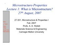
<strong>Microstructure</strong>-<strong>Properties</strong>: I<br />
Lecture 4B:<br />
Anisotropic Elasticity<br />
27-301<br />
Fall, 2007<br />
Prof. A. D. Rollett<br />
Processing<br />
Performance<br />
<strong>Microstructure</strong> <strong>Properties</strong>
2<br />
Objective<br />
Linear<br />
Ferromagnets<br />
Non-linear<br />
properties<br />
Electric.<br />
Conduct.<br />
Tensors<br />
Elasticity<br />
Symmetry<br />
Objective of Lecture 4B<br />
• The objective of this lecture is to provide a<br />
mathematical framework for the description of<br />
properties, especially when they vary with<br />
direction.<br />
• A basic property that occurs in almost<br />
applications is elasticity. Although elastic<br />
response is linear for all practical purposes, it<br />
is often anisotropic (composites, textured<br />
polycrystals etc.).
3<br />
Objective<br />
Linear<br />
Ferromagnets<br />
Non-linear<br />
properties<br />
Electric.<br />
Conduct.<br />
Tensors<br />
Elasticity<br />
Symmetry<br />
Linear properties<br />
• Certain properties, such as elasticity in<br />
most cases, are linear which means that<br />
we can simplify even further to obtain<br />
or if R 0 = 0,<br />
R = R 0 + PF<br />
R = PF.<br />
e.g. elasticity: σ = C ε<br />
stiffness<br />
In tension, C ≡ Young’s modulus, Y or E.
4<br />
Objective<br />
Linear<br />
Ferromagnets<br />
Non-linear<br />
properties<br />
Electric.<br />
Conduct.<br />
Tensors<br />
Elasticity<br />
Symmetry<br />
Elasticity<br />
• Elasticity: example of a property that requires tensors<br />
to describe it fully.<br />
• Even in cubic metals, a crystal is quite anisotropic.<br />
The [111] in many cubic metals is stiffer than the<br />
[100] direction.<br />
• Even in cubic materials, 3<br />
numbers/coefficients/moduli are required to describe<br />
elastic properties; isotropic materials only require 2.<br />
• Familiarity with Miller indices is assumed.
5<br />
Objective<br />
Linear<br />
Ferromagnets<br />
Non-linear<br />
properties<br />
Electric.<br />
Conduct.<br />
Tensors<br />
Elasticity<br />
Symmetry<br />
Elastic Anisotropy: 1<br />
• First we restate the linear elastic relations for<br />
the properties Compliance, written S, <strong>and</strong><br />
Stiffness, written C (!), which connect stress, σ<br />
, <strong>and</strong> strain, ε. We write it first in vector-tensor<br />
notation with “:” signifying inner product (i.e.<br />
add up terms that have a common suffix or<br />
index in them):<br />
σ = C:ε<br />
ε = S:σ<br />
• In component form (with suffixes),<br />
σ ij = C ijkl ε kl<br />
ε ij = S ijkl σ kl
6<br />
Objective<br />
Linear<br />
Ferromagnets<br />
Non-linear<br />
properties<br />
Electric.<br />
Conduct.<br />
Tensors<br />
Elasticity<br />
Symmetry<br />
Elastic Anisotropy: 2<br />
The definitions of the stress <strong>and</strong> strain tensors mean<br />
that they are both symmetric (second rank) tensors.<br />
Therefore we can see that<br />
ε 23 = S 2311 σ 11<br />
ε 32 = S 3211 σ 11 = ε 23<br />
which means that,<br />
S 2311 = S 3211<br />
<strong>and</strong> in general,<br />
S ijkl = S jikl<br />
We will see later on that this reduces considerably the<br />
number of different coefficients needed.
7<br />
Objective<br />
Linear<br />
Ferromagnets<br />
Non-linear<br />
properties<br />
Electric.<br />
Conduct.<br />
Tensors<br />
Elasticity<br />
Symmetry<br />
Stiffness in sample coords.<br />
• Consider how to express the elastic properties of a<br />
single crystal in the sample coordinates. In this case<br />
we need to rotate the (4 th rank) tensor from crystal<br />
coordinates to sample coordinates using the<br />
orientation (matrix), a (see lecture A):<br />
c ijkl ' = a im a jn a ko a lp c mnop<br />
• Note how the transformation matrix appears four<br />
times because we are transforming a 4th rank tensor!<br />
• The axis transformation matrix, a, is also written as λ.
8<br />
Objective<br />
Linear<br />
Ferromagnets<br />
Non-linear<br />
properties<br />
Electric.<br />
Conduct.<br />
Tensors<br />
Elasticity<br />
Symmetry<br />
Young’s modulus from compliance<br />
• Young's modulus as a function of direction<br />
can be obtained from the compliance tensor<br />
as E=1/s' 1111 . Using compliances <strong>and</strong> a stress<br />
boundary condition (only σ 11 ≠0) is most<br />
straightforward. To obtain s' 1111 , we simply<br />
apply the same transformation rule,<br />
s' ijkl = a im a jn a ko a lp s mnop
9<br />
Objective<br />
Linear<br />
Ferromagnets<br />
Non-linear<br />
properties<br />
Electric.<br />
Conduct.<br />
Tensors<br />
Elasticity<br />
Symmetry<br />
“matrix notation”<br />
• It is useful to re-express the three quantities<br />
involved in a simpler format. The stress <strong>and</strong><br />
strain tensors are vectorized, i.e. converted<br />
into a 1x6 notation <strong>and</strong> the elastic tensors are<br />
reduced to 6x6 matrices.<br />
"<br />
$<br />
#<br />
! 1 1 ! 1 2 ! 1 3<br />
! 2 1 ! 2 2 ! 2 3<br />
! 3 1 ! 3 2 ! 3 3<br />
%<br />
' ( )<br />
'<br />
&<br />
*<br />
"<br />
$<br />
#<br />
( * ) ( ! 1,! 2,! 3,! 4,! 5,! )<br />
6<br />
! 1 ! 6 ! 5<br />
! 6 ! 2 ! 4<br />
! 5 ! 4 ! 3<br />
%<br />
'<br />
&
10<br />
Objective<br />
Linear<br />
Ferromagnets<br />
Non-linear<br />
properties<br />
Electric.<br />
Conduct.<br />
Tensors<br />
Elasticity<br />
Symmetry<br />
“matrix notation”, contd.<br />
• Similarly for strain:<br />
"<br />
$<br />
#<br />
! 1 1 ! 1 2 ! 1 3<br />
! 2 1 ! 2 2 ! 2 3<br />
! 3 1 ! 3 2 ! 3 3<br />
The particular definition of shear strain used in the<br />
reduced notation happens to correspond to that used<br />
in mechanical engineering such that ε 4 is the change<br />
in angle between direction 2 <strong>and</strong> direction 3 due to<br />
deformation.<br />
%<br />
'<br />
&<br />
( ) *<br />
"<br />
$<br />
$<br />
#<br />
( * ) ( ! 1,! 2,! 3,! 4,! 5,! )<br />
6<br />
! 1<br />
1<br />
2 ! 6<br />
1<br />
2 ! 5<br />
1<br />
2 ! 6<br />
! 2<br />
1<br />
2 ! 4<br />
1<br />
2 ! 5<br />
1<br />
2 ! 4<br />
! 3<br />
%<br />
'<br />
'<br />
&
11<br />
Objective<br />
Linear<br />
Ferromagnets<br />
Non-linear<br />
properties<br />
Electric.<br />
Conduct.<br />
Tensors<br />
Elasticity<br />
Symmetry<br />
Work conjugacy, matrix inversion<br />
• The more important consideration is that the<br />
reason for the factors of two is so that work<br />
conjugacy is maintained.<br />
dW = σ:dε = σ ij : dε ij = σ k • dε k<br />
Also we can combine the expressions<br />
σ = Cε <strong>and</strong> ε = Sσ to give:<br />
σ = CSσ, which shows:<br />
I = CS, or, C = S -1
12<br />
Objective<br />
Linear<br />
Ferromagnets<br />
Non-linear<br />
properties<br />
Electric.<br />
Conduct.<br />
Tensors<br />
Elasticity<br />
Symmetry<br />
Tensor conversions: stiffness<br />
• Lastly we need a way to convert the tensor<br />
coefficients of stiffness <strong>and</strong> compliance to the<br />
matrix coefficients. For stiffness, it is very<br />
simple because one substitutes values<br />
according to the following table, such that<br />
matrix C11 = tensor C 1111 for example.<br />
Tensor 11 22 33 23 32 13 31 12 21<br />
Matrix 1 2 3 4 4 5 5 6 6
13<br />
Objective<br />
Linear<br />
Ferromagnets<br />
Non-linear<br />
properties<br />
Electric.<br />
Conduct.<br />
Tensors<br />
Elasticity<br />
Symmetry<br />
C =<br />
!<br />
#<br />
#<br />
#<br />
#<br />
#<br />
#<br />
#<br />
"<br />
Stiffness Matrix<br />
C 1 1 C 1 2 C 1 3 C 1 4 C 1 5 C 1 6<br />
C 2 1 C 2 2 C 2 3 C 2 4 C 2 5 C 2 6<br />
C 3 1 C 3 2 C 3 3 C 3 4 C 3 5 C 3 6<br />
C 4 1 C 4 2 C 4 3 C 4 4 C 4 5 C 4 6<br />
C 5 1 C 5 2 C 5 3 C 5 4 C 5 5 C 5 6<br />
C 6 1 C 6 2 C 6 3 C 6 4 C 6 5 C 6 6<br />
$<br />
&<br />
&<br />
&<br />
&<br />
&<br />
&<br />
&<br />
%
14<br />
Objective<br />
Linear<br />
Ferromagnets<br />
Non-linear<br />
properties<br />
Electric.<br />
Conduct.<br />
Tensors<br />
Elasticity<br />
Symmetry<br />
Tensor conversions: compliance<br />
• For compliance some factors of two are<br />
required <strong>and</strong> so the rule becomes:<br />
pS = S ijkl mn<br />
p =1 m AND n " [ 1,2,3 ]<br />
p = 2 m XOR n " [ 1,2,3 ]<br />
p = 4 m AND n " [ 4,5,6]
15<br />
Objective<br />
Linear<br />
Ferromagnets<br />
Non-linear<br />
properties<br />
Electric.<br />
Conduct.<br />
Tensors<br />
Elasticity<br />
Symmetry<br />
Relationships between coefficients:<br />
C in terms of S<br />
Some additional useful relations between coefficients<br />
for cubic materials are as follows. Symmetrical<br />
relationships exist for compliances in terms of<br />
stiffnesses (next slide).<br />
C 11 = (S 11 +S 12 )/{(S 11 -S 12 )(S 11 +2S 12 )}<br />
C 12 = -S 12 /{(S 11 -S 12 )(S 11 +2S 12 )}<br />
C 44 = 1/S 44 .
16<br />
Objective<br />
Linear<br />
Ferromagnets<br />
Non-linear<br />
properties<br />
Electric.<br />
Conduct.<br />
Tensors<br />
Elasticity<br />
Symmetry<br />
S in terms of C<br />
The relationships for S in terms of C are symmetrical to<br />
those for stiffnesses in terms of compliances (a<br />
simple exercise in algebra!).<br />
S 11 = (C 11 +C 12 )/{(C 11 -C 12 )(C 11 +2C 12 )}<br />
S 12 = -C 12 /{(C 11 -C 12 )(C 11 +2C 12 )}<br />
S 44 = 1/C 44 .
17<br />
Effect of symmetry on stiffness matrix<br />
Objective<br />
Linear<br />
Ferromagnets<br />
Non-linear<br />
properties<br />
Electric.<br />
Conduct.<br />
Tensors<br />
Elasticity<br />
Symmetry<br />
• Why do we need to look at the effect of symmetry?<br />
For a cubic material, only 3 independent coefficients<br />
are needed as opposed to the 81 coefficients in a 4th<br />
rank tensor. The reason for this is the symmetry of<br />
the material.<br />
• What does symmetry mean? Fundamentally, if you<br />
pick up a crystal, rotate [mirror] it <strong>and</strong> put it back<br />
down, then a symmetry operation [rotation, mirror] is<br />
such that you cannot tell that anything happened.<br />
• From a mathematical point of view, this means that<br />
the property (its coefficients) does not change. For<br />
example, if the symmetry operator changes the sign<br />
of a coefficient, then it must be equal to zero.
18<br />
Effect of symmetry on stiffness matrix<br />
Objective<br />
Linear<br />
Ferromagnets<br />
Non-linear<br />
properties<br />
Electric.<br />
Conduct.<br />
Tensors<br />
Elasticity<br />
Symmetry<br />
• Following Reid, p.66 et seq.:<br />
Apply a 90° rotation about the crystal-z axis<br />
(axis 3),<br />
C’ ijkl = O im O jn O ko O lp C mnop :<br />
C’ = C<br />
C ! =<br />
#<br />
%<br />
%<br />
%<br />
%<br />
%<br />
%<br />
%<br />
%<br />
$ %<br />
O 4 z =<br />
C 22 C 21 C 23 C 25 "C 24 "C 26<br />
C 21 C 11 C 13 C 15 "C 14 "C 16<br />
C 23 C 13 C 33 C 35 "C 34 "C 36<br />
C 25 C 15 C 35 C 55 "C 54 "C 56<br />
"C 24 "C 14 "C 34 "C 54 C 44 C 46<br />
"C 26 "C 16 "C 36 "C 56 C 46 C 66<br />
" 0 !1 0%<br />
$ '<br />
$ 1 0 0'<br />
$ '<br />
# 0 0 1&<br />
&<br />
(<br />
(<br />
(<br />
(<br />
(<br />
(<br />
(<br />
(<br />
' (
19<br />
Objective<br />
Linear<br />
Ferromagnets<br />
Non-linear<br />
properties<br />
Electric.<br />
Conduct.<br />
Tensors<br />
Elasticity<br />
Symmetry<br />
Effect of symmetry, 2<br />
• Using P’ = P, we can equate coefficients <strong>and</strong><br />
find that:<br />
C 11 =C 22 , C 13 =C 23, C 44 =C 35 , C 16 =-C 26,<br />
C 14 =C 15 = C 24 = C 25 = C 34 = C 35 = C 36 = C 45 = C 46<br />
= C 56 = 0.<br />
C ! =<br />
# C1 1 C1 2 C1 3 0 0 C1 6 &<br />
% C1 2 C1 1 C1 3 0 0 "C1 6(<br />
% C1 3<br />
% 0<br />
%<br />
0<br />
%<br />
$ C1 6<br />
C1 3<br />
0<br />
0<br />
"C1 6<br />
C3 3<br />
0<br />
0<br />
0<br />
0<br />
C4 4<br />
0<br />
0<br />
0<br />
0<br />
C4 4<br />
C4 6<br />
0<br />
0<br />
C4 6<br />
C6 6<br />
(<br />
(<br />
(<br />
(<br />
'
20<br />
Objective<br />
Linear<br />
Ferromagnets<br />
Non-linear<br />
properties<br />
Electric.<br />
Conduct.<br />
Tensors<br />
Elasticity<br />
Symmetry<br />
Effect of symmetry, 3<br />
• Thus by repeated applications of the<br />
symmetry operators, one can demonstrate<br />
(for cubic crystal symmetry) that one can<br />
reduce the 81 coefficients down to only 3<br />
independent quantities. These become two in<br />
the case of isotropy.<br />
! C11 C12 C12 0 0 0 $<br />
#<br />
&<br />
# C12 C11 C12 0 0 0 &<br />
#<br />
&<br />
# C12 C12 C11 0 0 0 &<br />
#<br />
0 0 0 C44 0 0<br />
&<br />
#<br />
&<br />
# 0 0 0 0 C44 0 &<br />
#<br />
&<br />
" # 0 0 0 0 0 C44% &
21<br />
Objective<br />
Linear<br />
Ferromagnets<br />
Non-linear<br />
properties<br />
Electric.<br />
Conduct.<br />
Tensors<br />
Elasticity<br />
Symmetry<br />
Cubic crystals: anisotropy factor<br />
• If one applies the symmetry elements of<br />
the cubic system, it turns out that only<br />
three independent coefficients remain: C 11 ,<br />
C 12 <strong>and</strong> C 44 , (similar set for compliance).<br />
From these three, a useful combination of<br />
the first two is<br />
C' = (C 11 - C 12 )/2<br />
• See Nye, Physical <strong>Properties</strong> of Crystals
22<br />
Objective<br />
Linear<br />
Ferromagnets<br />
Non-linear<br />
properties<br />
Electric.<br />
Conduct.<br />
Tensors<br />
Elasticity<br />
Symmetry<br />
Zener’s anisotropy factor<br />
• C' = (C 11 - C 12 )/2 turns out to be the stiffness<br />
associated with a shear in a direction<br />
on a plane. In certain martensitic<br />
transformations, this modulus can approach<br />
zero which corresponds to a structural<br />
instability. Zener proposed a measure of<br />
elastic anisotropy based on the ratio C 44 /C'.<br />
This turns out to be a useful criterion for<br />
identifying materials that are elastically<br />
anisotropic.
23<br />
Objective<br />
Linear<br />
Ferromagnets<br />
Non-linear<br />
properties<br />
Electric.<br />
Conduct.<br />
Tensors<br />
Elasticity<br />
Symmetry<br />
Rotated compliance (matrix)<br />
• Given an orientation a ij , we transform the<br />
compliance tensor, using cubic point group<br />
symmetry, <strong>and</strong> find that:<br />
S 1! 1 = S1 1 a1 1<br />
( 4 4 4<br />
+ a1<br />
2 + ) a1<br />
3<br />
+ 2S 1 2 a 1 2<br />
( 2 2 2 2 2 2<br />
a1 3 + a1 1a1<br />
2 + ) a1 1a1<br />
3<br />
( )<br />
2 2 2 2 2 2<br />
+ S4 4 a1 2a1<br />
3 + a1 1a1<br />
2 + a1 1a1<br />
3
24<br />
Objective<br />
Linear<br />
Ferromagnets<br />
Non-linear<br />
properties<br />
Electric.<br />
Conduct.<br />
Tensors<br />
Elasticity<br />
Symmetry<br />
Rotated compliance (matrix)<br />
• This can be further simplified with the aid of the<br />
st<strong>and</strong>ard relations between the direction cosines,<br />
a ik a jk = 1 for i=j; a ik a jk = 0 for i≠j, (a ik a jk = δ ij ) to read as<br />
follows.<br />
s 1! 1 = s1 1 "<br />
2( s1 1 " s1 2 " 1<br />
2<br />
s ) 4 4 # 1<br />
{ 2 2 2 2 2 2<br />
#2 + # 2#3<br />
+ }<br />
#3#1<br />
• By definition, the Young’s modulus in any direction is<br />
given by the reciprocal of the compliance, E = 1/S’ 11.
25<br />
Objective<br />
Linear<br />
Ferromagnets<br />
Non-linear<br />
properties<br />
Electric.<br />
Conduct.<br />
Tensors<br />
Elasticity<br />
Symmetry<br />
Anisotropy in cubic materials<br />
• Thus the second term on the RHS is zero for <br />
directions <strong>and</strong>, for C 44 /C'>1, a maximum in <br />
directions (conversely<br />
a minimum for C 44 /C'
26<br />
Objective<br />
Linear<br />
Ferromagnets<br />
Non-linear<br />
properties<br />
Electric.<br />
Conduct.<br />
Tensors<br />
Elasticity<br />
Symmetry<br />
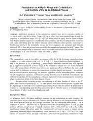
Stiffness coefficients, cubics<br />
[Courtney]
27<br />
Objective<br />
Linear<br />
Ferromagnets<br />
Non-linear<br />
properties<br />
Electric.<br />
Conduct.<br />
Tensors<br />
Elasticity<br />
Symmetry<br />
Anisotropy in terms of moduli<br />
• Another way to write the above equation is to<br />
insert the values for the Young's modulus in<br />
the soft <strong>and</strong> hard directions, assuming that<br />
the are the most compliant<br />
direction(s). (Courtney uses α, β, <strong>and</strong> γ in<br />
place of my α 1 , α 2 , <strong>and</strong> α 3 .) The advantage of<br />
this formula is that moduli in specific<br />
directions can be used directly.<br />
1<br />
E uvw<br />
= 1<br />
E 100<br />
"<br />
! 3#<br />
$<br />
1<br />
E 100<br />
&<br />
E111' ( 2 2 2 2 2 2<br />
1(<br />
2 + (2(<br />
3<br />
+(3 (1<br />
! 1<br />
%<br />
( )
28<br />
Objective<br />
Linear<br />
Ferromagnets<br />
Non-linear<br />
properties<br />
Electric.<br />
Conduct.<br />
Tensors<br />
Elasticity<br />
Symmetry<br />
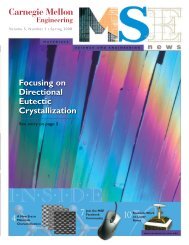
Example Problem<br />
Should be E = 18.89
29<br />
Objective<br />
Linear<br />
Ferromagnets<br />
Non-linear<br />
properties<br />
Electric.<br />
Conduct.<br />
Tensors<br />
Elasticity<br />
Symmetry<br />
Summary<br />
• We have covered the following topics:<br />
– Linear properties<br />
– Non-linear properties<br />
– Examples of properties<br />
– Tensors, vectors, scalars.<br />
– Magnetism, example of linear (permeability), nonlinear<br />
(magnetization curve) with strong<br />
microstructural influence.<br />
– Elasticity, as example as of higher order property,<br />
also as example as how to apply (crystal)<br />
symmetry.
30<br />
Objective<br />
Linear<br />
Ferromagnets<br />
Non-linear<br />
properties<br />
Electric.<br />
Conduct.<br />
Tensors<br />
Elasticity<br />
Symmetry<br />
Supplemental Slides<br />
• The following slides contain some useful<br />
material for those who are not familiar with all<br />
the detailed mathematical methods of<br />
matrices, transformation of axes etc.
31<br />
Objective<br />
Linear<br />
Ferromagnets<br />
Non-linear<br />
properties<br />
Electric.<br />
Conduct.<br />
Tensors<br />
Elasticity<br />
Symmetry<br />
Notation<br />
F Stimulus (field)<br />
R Response<br />
P Property<br />
j electric current<br />
E electric field<br />
D electric polarization<br />
ε Strain<br />
σ Stress (or conductivity)<br />
ρ Resistivity<br />
d piezoelectric tensor<br />
C elastic stiffness<br />
S elastic compliance<br />
a rotation matrix<br />
W work done (energy)<br />
I identity matrix<br />
O<br />
Y Young’s Young s modulus<br />
δ Kronecker delta<br />
e axis (unit) vector<br />
T tensor<br />
αα direction cosine<br />
symmetry operator (matrix)
32<br />
Objective<br />
Linear<br />
Ferromagnets<br />
Non-linear<br />
properties<br />
Electric.<br />
Conduct.<br />
Tensors<br />
Elasticity<br />
Symmetry<br />
Bibliography<br />
• R.E. Newnham, <strong>Properties</strong> of <strong>Materials</strong>: Anisotropy, Symmetry, Structure, Oxford University<br />
Press, 2004, 620.112 N55P.<br />
• De Graef, M., lecture notes for 27-201.<br />
• Nye, J. F. (1957). Physical <strong>Properties</strong> of Crystals. Oxford, Clarendon Press.<br />
• T. Courtney, Mechanical Behavior of <strong>Materials</strong>, McGraw-Hill, 0-07-013265-8, 620.11292<br />
C86M.<br />
• Chen, C.-W. (1977). Magnetism <strong>and</strong> metallurgy of soft magnetic materials. New York,<br />
Dover.<br />
• Chikazumi, S. (1996). Physics of Ferromagnetism. Oxford, Oxford University Press.<br />
• Attwood, S. S. (1956). Electric <strong>and</strong> Magnetic Fields. New York, Dover.<br />
• Newey, C. <strong>and</strong> G. Weaver (1991). <strong>Materials</strong> Principles <strong>and</strong> Practice. Oxford, Engl<strong>and</strong>,<br />
Butterworth-Heinemann.<br />
• Kocks, U. F., C. Tomé, et al., Eds. (1998). Texture <strong>and</strong> Anisotropy, Cambridge University<br />
Press, Cambridge, UK.<br />
• Reid, C. N. (1973). Deformation Geometry for <strong>Materials</strong> Scientists. Oxford, UK, Pergamon.<br />
• Braithwaite, N. <strong>and</strong> G. Weaver (1991). Electronic <strong>Materials</strong>. The Open University, Engl<strong>and</strong>,<br />
Butterworth-Heinemann.
33<br />
Objective<br />
Linear<br />
Ferromagnets<br />
Non-linear<br />
properties<br />
Electric.<br />
Conduct.<br />
Tensors<br />
Elasticity<br />
Symmetry<br />
Mathematical Descriptions<br />
• Mathematical descriptions of properties are available.<br />
• Mathematics, or a type of mathematics provides a<br />
quantitative framework. It is always necessary,<br />
however, to make a correspondence between<br />
mathematical variables <strong>and</strong> physical quantities.<br />
• In group theory one might say that there is a set of<br />
mathematical operations & parameters, <strong>and</strong> a set of<br />
physical quantities <strong>and</strong> processes: if the mathematics<br />
is a good description, then the two sets are<br />
isomorphous.
34<br />
Objective<br />
Linear<br />
Ferromagnets<br />
Non-linear<br />
properties<br />
Electric.<br />
Conduct.<br />
Tensors<br />
Elasticity<br />
Symmetry<br />
Non-Linear properties, example<br />
• Another important example of non-linear properties is plasticity,<br />
i.e. the irreversible deformation of solids.<br />
• A typical description of the response at plastic yield<br />
(what happens when you load a material to its yield stress)<br />
is elastic-perfectly plastic. In other<br />
words, the material responds<br />
elastically until the yield stress is<br />
reached, at which point the stress<br />
remains constant (strain rate<br />
unlimited).<br />
• A more realistic description is a power-law with<br />
a large exponent, n~50. The stress is scaled by<br />
the crss, <strong>and</strong> be expressed as either shear stressshear<br />
strain rate [graph], or tensile stress-tensile<br />
strain [equation].<br />
˙<br />
! =<br />
# " &<br />
% (<br />
$ " yield '<br />
n
35<br />
Objective<br />
Linear<br />
Ferromagnets<br />
Non-linear<br />
properties<br />
Electric.<br />
Conduct.<br />
Tensors<br />
Elasticity<br />
Symmetry<br />
Einstein Convention<br />
• The Einstein Convention, or summation rule<br />
for suffixes looks like this:<br />
A i = B ij C j<br />
where “i” <strong>and</strong> “j” both are integer indexes<br />
whose range is {1,2,3}. So, to find each “i th ”<br />
component of A on the LHS, we sum up over<br />
the repeated index, “j”, on the RHS:<br />
A 1 = B 11 C 1 + B 12 C 2 + B 13 C 3<br />
A 2 = B 21 C 1 + B 22 C 2 + B 23 C 3<br />
A 3 = B 31 C 1 + B 32 C 2 + B 33 C 3
36<br />
Objective<br />
Linear<br />
Ferromagnets<br />
Non-linear<br />
properties<br />
Electric.<br />
Conduct.<br />
Tensors<br />
Elasticity<br />
Symmetry<br />
Matrix Multiplication<br />
• Take each row of the LH matrix in turn <strong>and</strong><br />
multiply it into each column of the RH matrix.<br />
• In suffix notation, a ij = b ikc kj<br />
( a! + b" + c# a$ + b% + cµ a# + b& + c' +<br />
*<br />
-<br />
* d! + e" + f# d$ + e% + fµ d# + e& + f' -<br />
*<br />
-<br />
) l! + m" + n# l$ + m% + nµ l# + m& + n',<br />
=<br />
( a b c +<br />
* -<br />
* d e f -<br />
* -<br />
) l m n,<br />
.<br />
( ! $ # +<br />
* -<br />
* " % & -<br />
* -<br />
) / µ ' ,
37<br />
Objective<br />
Linear<br />
Ferromagnets<br />
Non-linear<br />
properties<br />
Electric.<br />
Conduct.<br />
Tensors<br />
Elasticity<br />
Symmetry<br />
<strong>Properties</strong> of Rotation Matrix<br />
• The rotation matrix is an orthogonal matrix, meaning<br />
that any row is orthogonal to any other row (the dot<br />
products are zero). In physical terms, each row<br />
represents a unit vector that is the position of the<br />
corresponding (new) old axis in terms of the (old)<br />
new axes.<br />
• The same applies to columns: in suffix notation -<br />
a ija kj = δ ik , a jia jk = δ ik<br />
! a b c$<br />
# &<br />
# d e f &<br />
# &<br />
" l m n%<br />
bc+ef+mn = 0<br />
ad+be+cf = 0
38<br />
Objective<br />
Linear<br />
Ferromagnets<br />
Non-linear<br />
properties<br />
Electric.<br />
Conduct.<br />
Tensors<br />
Elasticity<br />
Symmetry<br />
Matrix<br />
representation<br />
of the rotation<br />
point groups<br />
Kocks: Ch. 1 Table II
39<br />
Objective<br />
Linear<br />
Ferromagnets<br />
Non-linear<br />
properties<br />
Electric.<br />
Conduct.<br />
Tensors<br />
Elasticity<br />
Symmetry<br />
Homogeneity<br />
• Stimuli <strong>and</strong> responses of interest are, in general, not scalar quantities<br />
but tensors. Furthermore, some of the properties of interest, such as<br />
the plastic properties of a material, are far from linear at the scale of a<br />
polycrystal. Nonetheless, they can be treated as linear at a suitably<br />
local scale <strong>and</strong> then an averaging technique can be used to obtain the<br />
response of the polycrystal. The local or microscopic response is<br />
generally well understood but the validity of the averaging techniques is<br />
still controversial in many cases. Also, we will only discuss cases<br />
where a homogeneous response can be reasonably expected.<br />
• There are many problems in which a non-homogeneous response to a<br />
homogeneous stimulus is of critical importance. Stress-corrosion<br />
cracking, for example, is a wildly non-linear, non-homogeneous<br />
response to an approximately uniform stimulus which depends on the<br />
mechanical <strong>and</strong> electro-chemical properties of the material.
40<br />
Objective<br />
Linear<br />
Ferromagnets<br />
Non-linear<br />
properties<br />
Electric.<br />
Conduct.<br />
Tensors<br />
Elasticity<br />
Symmetry<br />
The “RVE”<br />
• In order to describe the properties of a<br />
material, it is useful to define a representative<br />
volume element (RVE) that is large enough to<br />
be statistically representative of that region<br />
(but small enough that one can subdivide a<br />
body).<br />
• For example, consider a polycrystal: how<br />
many grains must be included in order for the<br />
element to be representative of that point in<br />
the material?
41<br />
Objective<br />
Linear<br />
Ferromagnets<br />
Non-linear<br />
properties<br />
Electric.<br />
Conduct.<br />
Tensors<br />
Elasticity<br />
Symmetry<br />
Transformations of Stress & Strain Vectors<br />
!<br />
• It is useful to be able to transform the axes<br />
of stress tensors when written in vector<br />
form (equation on the left). The table<br />
(right) is taken from Newnham’s book. In<br />
vector-matrix form, the transformations<br />
are:<br />
$ # 1"<br />
' +<br />
& ) -<br />
&<br />
# " 2)<br />
-<br />
& # " ) - 3<br />
& ) = -<br />
&<br />
# " 4)<br />
-<br />
& # " 5)<br />
-<br />
& )<br />
% # "<br />
-<br />
6(<br />
,<br />
* 11 * 12 * 13 * 14 * 15 * 16<br />
* 21 * 22 * 23 * 24 * 25 * 26<br />
* 31 * 32 * 33 * 34 * 35 * 36<br />
* 41 * 42 * 43 * 44 * 45 * 46<br />
* 51 * 52 * 53 * 54 * 55 * 56<br />
* 61 * 62 * 63 * 64 * 65 * 66<br />
. $ # ' 1<br />
0 & )<br />
0 &<br />
# 2)<br />
0 & # ) 3<br />
0 & )<br />
0 &<br />
# 4)<br />
0 & # 5)<br />
0 & )<br />
/ % # 6(<br />
!<br />
"<br />
# i = $ ij# j<br />
%1<br />
# i = $ ij<br />
# " j<br />
%1T<br />
& " i = $ ij & j<br />
T<br />
&i = $ ij&<br />
" j