Automated Synthesis of Body Schema using Multiple Sensor ...

Automated Synthesis of Body Schema using Multiple Sensor Modalities
Abstract
The way in which organisms create body schema, based on
their interactions with the real world, is an unsolved problem
in neuroscience. Similarly, in evolutionary robotics, a
robot learns to behave in the real world either without recourse
to an internal model (requiring at least hundreds of interactions),
or a model is hand designed by the experimenter
(requiring much prior knowledge about the robot and its environment).
In this paper we present a method that allows a
physical robot to automatically synthesize a body schema, using
multimodal sensor data that it obtains through interaction
with the real world. Furthermore, this synthesis can be either
parametric (the experimenter provides an approximate model
and the robot then refines the model) or topological: the robot
synthesizes a predictive model of its own body plan using little
prior knowledge. We show that this latter type of synthesis
can occur when a physical quadrupedal robot performs only
nine, 5-second interactions with its environment.
The question of whether organisms do, or robots should,
create and maintain models of themselves are central questions
in neuroscience and robotics respectively. In neuroscience,
it has been argued that higher organisms must possess
predictive models of their own bodies, because biological
sensor systems are too slow to provide adequate feedback
for fast and/or complex movements: internal models
must predict what movements will result from a set of muscle
contractions (D. Wolpert, 1998; Llinas, 2001). To this
end, neural imaging and behavioral studies have begun to
seek out where in the primate brain such models may exist,
and what form they take (D. Wolpert, 1998; Bhushan and
Shadmehr, 1999; Imamizu et al., 2003).
In a similar way, internal models lie at the heart of a longstanding
debate in artificial intelligence and robotics: how,
or should a robot rely on internal models to realize useful behaviors?
In the early decades of AI modeling played a large
role, when research emphasized higher-level cognitive functions,
such as planning. Brooks (Brooks, 1991) and later
others (Hendriks-Jansen, 1996; Clark, 1998; Pfeifer and
Scheier, 1999) spearheaded embodied AI, in which modelfree
embodied robots were emphasized: it was thought that
active interaction with the environment could supplant the
need for internal introspection using models.
Josh Bongard, Victor Zykov and Hod Lipson
Computational Synthesis Laboratory
Sibley School of Mechanical and Aerospace Engineering
Cornell University, Ithaca, NY, 14853
[josh.bongard | viktor.zykov | hod.lipson]@cornell.edu
This paper, along with previous work (Bongard and Lipson,
2005b), introduces a methodology that integrates introspective
modeling and reactive embodied behavior. We refer
to this method as the estimation-exploration algorithm, or
EEA: the EEA is a co-evolutionary algorithm that maintains
populations of models and populations of tests. A simplified
schematic of the EEA is shown in Figure 1. The algorithm
is iterative: models are synthesized based on the sensorial
experiences of an embodied and situated robot, and those
models are in turn used to derive new controllers that, when
executed on the physical robot, generate new sensor data for
further model synthesis (see (Bongard and Lipson, 2005b)
for an overview).
By using a model to derive a controller, the number of
physical interactions that the robot must perform can be reduced
by orders of magnitude (Keymeulen et al., 1998): if a
controller is learned or evolved on a physical robot, at least
hundreds of evaluations are required. However, if a model is
not accurate, behaviors may not transfer from simulation to
reality. This is known as the infamous “reality gap” problem
(Jakobi, 1997), and several methods have been proposed to
overcome it, such as adding noise to the simulated robot’s
sensors (Jakobi, 1997); adding generic safety margins to
the simulated objects comprising the physical system (Funes
and Pollack, 1999); evolving first in simulation followed by
further adaptation on the physical robot (Pollack et al., 2000;
Mahdavi and Bentley, 2003); or implementing some neural
plasticity that allows the physical robot to adapt during its
lifetime to novel environments (Floreano and Urzelai, 2001;
DiPaolo, 2000; Tokura et al., 2001).
Keymeulen et. al’s work (Keymeulen et al., 1998) represents
the closet method to the one described here. In that
work, a model is synthesized based on sensor feedback from
the robot’s interaction with its environment. A model is
learned as a wheeled robot learns to perform a behavior;
the model is a set of passively obtained instances of sensor
changes resulting from motor commands. However, there is
no transformation or compression of this data into a general
or explicit model of the robot or its environment. For example,
in that work the robot would not be able to distinguish

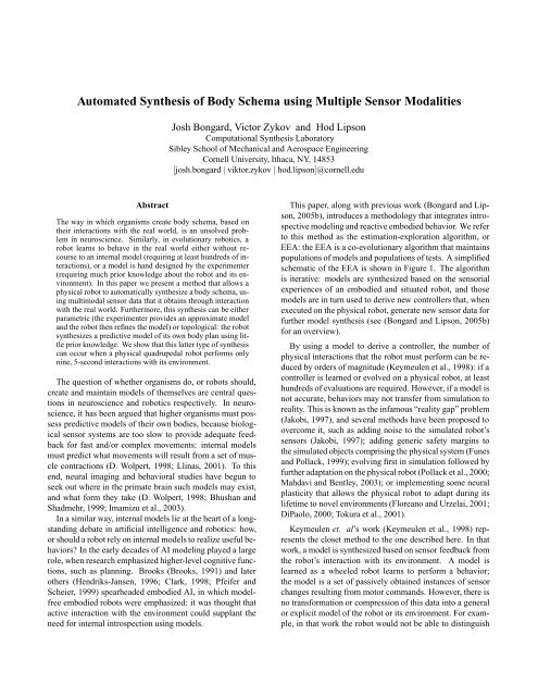
a
b
Figure 1: The physical robot targeted for automated identification.
between its left and right wheels, because it has no explicit
model of its own body; it can only predict, in environmental
contexts that it has already encountered, what might happen
if it sends a motor command to its wheel. In contrast, the
EEA actively generates explicit models based on incoming
sensor data (such as shown in Figure 5). Here, we present
validation of our algorithm on a physical articulated robot
(shown in Figure 1a): the robot evolves an explicit model of
its body using sensor data from different modalities. This
is the first time explicit, predictive robot models have been
intelligently synthesized based on physical interactions.
In the next section the methodology is described, which
includes description of the target robot, the space of models
and the space of controllers, and how these spaces are
searched. Then, results from both parametric and topological
identification of the robot are presented; the final section
provides some discussion and concluding remarks.
Methods
In previous work we have documented the ability of the EEA
to parametrically identify a simulated target robot, given
some initial approximate model of it (Bongard and Lipson,
2005b). In other problem domains we have demonstrated
that the EEA can synthesize both the topology and param-
eters of a hidden system, in which no model is required a
priori (Bongard and Lipson, 2005a). In order to apply the
EEA to a new target system, such as the physical robot used
in this work, three preparatory steps must be first carried out:
characterization of the system to be identified, how models
are to be represented and optimized, and how controllers are
to be represented and optimized.
Characterizing the Target System
The target system in this study is a quadrupedal, articulated
robot with eight actuated degrees of freedom. The robot consists
of a rectangular body and four legs attached to it with
hinge joints on each of the four sides of the robot’s body.
Each leg in turn is composed of an upper and lower leg, attached
together with a hinge joint. All eight hinge joints
of the robot are actuated with Airtronics 94359 high torque
servomotors. However, in the current study, the robot was
simplified by assuming that the knee joints are frozen: all
four legs are held straight when the robot is commanded to
perform some action. Table 1 gives the overall dimensions
of the robot’s parts.
Parameter Value (mm)
Width and length of the body 140
Height of the body 85
Length of the upper leg 95
Height of the upper leg 26
Length of the lower leg 125
Diameter of the foot 12
Table 1: Physical dimensions of the robot.
All eight servomotors are controlled using an on-board
PC-104 computer via a serial servo control board SV-203B,
which converts serial commands into pulse-width modulated
signals. Servo drives are capable of producing a maximum
of 200 ounce-inches of torque and 60 degrees per second of
speed. The actuation ranges for all of the robot’s joints are
summarized in table 2.
Lower range bound Upper range bound
(degrees) (degrees)
Hip joint -96 +74
Knee joint -96 +94
Table 2: Joint properties of the robot. Ranges are given relative
to the robot body for the hip joints, and relative to the
upper legs for the knee joints. Positive numbers indicate upward
motion; negative values indicate downward motion.
The robot is equipped with a suite of different sensors
polled by a 16-bit 32- channel PC-104 Diamond MM-32X-
AT data acquisition board. For the current identification
task, three sensor modalities were used: an external sensor
was used to determine the left/right and forward/back

tilt of the robot; four binary values indicated whether a foot
was touching the ground or not; and one value indicated the
clearance distance from the robot’s underbelly to the ground,
along the normal to its lower body surface. All sensor readings
were conducted manually, however all three kinds of
signals will be recorded in future by on-board accelerometers,
the strain gauges built into the lower legs, and an optical
distance sensor placed on the robot’s belly.
Characterizing the Space of Models
Models are considered to be three-dimensional simulations
of the physical robot (see Figure 5 for three model examples).
The simulations are created within Open Dynamics
Engine 1 , a three-dimensional dynamics simulator. However
in the current work only static identification is performed:
the physical robot is commanded to achieve a static pose,
and then hold still while sensor data is taken. Every candidate
model (as well as the target robot) is assumed to start
as a planar configuration of parts; when it begins to move, it
can assume a three-dimensional configuration. The geometry
and physical properties of the main body part is assumed
to be known; the eight upper and lower leg parts are represented
as solid cylinders. Each model is evaluated for an
arbitrarily set time of 300 time steps of the simulator, which
is enough time for most models to come to rest given an
arbitrary motor program.
Models are encoded as either vectors or matrices, and
these data structures are used to construct a possible articulated
robot in the simulation environment. In the first set
of experiments, we assume that everything about the physical
robot is known except the lengths of its four legs. Models
are therefore encoded as vectors containing eight real-valued
parameters in [0,1], with each value encoding the estimated
length of one of the eight leg parts. We constrain the estimation
about the minimum and maximum length of a leg to
be between 2 and 40 centimeters, so each value is scaled to
a real-value in [1,20]cm.
In the second set of results, we assume that less information
about the robot is known: how the eight body parts attach
to each other or the main body, and how the hinge joints
connecting them are oriented. In that case, models are encoded
as 8 × 4 real-valued matrices. Each row corresponds
to one of the eight parts. The first value in row i is scaled to
an integer in [0,i−1], indicating which of the previous body
parts it attaches to; the second value is scaled to an integer in
[0,3], indicating whether the current part attaches to the left,
front, right, or back side of the parental part. The third value
is scaled to an integer in [0,5], and indicates how the hinge
joint connecting the current part to its parent operates: 0 and
1 cause the part to rotate leftward or rightward in response
to a positive commanded joint angle (and rightward and leftward
in response to a negative commanded angle); 2 and 3
1 http://ode.org
cause the joint to rotate upward or downward in response to
a positive commanded angle; and 4 and 5 cause the part to
rotate leftward or rightward around its own axis in response
to a positive commanded angle. The fourth value is scaled
to a value in [1,20]cm to represent the length of the leg part.
In both types of experiments, a genetic algorithm using
deterministic crowding (Mahfoud, 1995) is used to optimize
the models. Genomes in the population are simply the vectors
or matrices described above. The subjective error of encoded
models is minimized by the genetic algorithm. Subjective
error is given as the error between the sensor values
obtained from the physical robot, and those obtained from
the simulated one:
e = v +
4
i=1
|t (t)
i − m(t) i | +
2
j=1
|t (l)
j − m(l) j | + 10|t(c) − m (c) |,
where e is the error of the model; v indicates the linear velocity
of the model robot (sometimes models do not come to
rest); t (t)
i indicates whether leg i touched the ground for the
target robot; m (t)
i indicates whether leg i touched the ground
for the model robot; t (l)
j indicates how much (in degrees) the
main body of the target robot was tilted away in relation to
gravity ( j = 1 for left/right tilt; j = 2 for forward/back tilt);
m (l)
j indicates how much the main body of the model was
tilted; t (c) indicates the clearance (in meters) from the target
robot’s belly to the ground; and m (c) indicates the clearance
for the model robot. By minimizing v, we select models that
come to rest within the alloted time. The clearance sensor
difference is amplified because it is reported in meters, and
for most poses achieved by the physical robot this value is
very small compared to the other terms. As can be seen in
Figure 1b, after the second set of sensor data has been obtained
from the target robot, there are two (or more) sets of
sensor data to be matched by a given model; in this case, the
subjective error of a model becomes
e = max{e1,e2,...en},
where ek indicates the error of the model using motor program
and sensor data set k from the physical robot.
In the first pass through the estimation phase, a random
population of models is generated, and optimized for
a fixed number of generations. On the second and subsequent
passes through the estimation phase, the previously
optimized population of models is used as the starting point,
but they are re-evaluated according to the new error metric
with the additional set of sensor data.
Characterizing the Space of Controllers
In this work a motor program is a set of four joint angles that
either the target robot, or a model robot, is commanded to
achieve 2 . Both the target and model robots begin in a planar
2 The four elbow joints are locked for these experiments.

a
b
c
d
Subjective Error
Total Length of Leg (cm)
Subjective Error
Total Length of Leg (cm)
40
30
20
10
8
6
4
3
2
0
40
10 20
Generation
30 40
35
30
25
20
15
10
5
40
30
20
10
8
6
0 10 20 30 40
Generation
4
3
2
0
40
10 20
Generation
30 40
35
30
25
20
15
10
5
0 10 20 30 40
Generation
Figure 2: Results from two runs of parametric identification.
a: The subjective error of each model. Model error
is calculated using touch, tilt and clearance sensor data. b:
The estimated leg lengths from the best model after each
generation from the same run. (Dots=target leg length; left
arrow=left leg, right arrow=right leg, up arrow=forward leg,
and down arrow=back leg.) c: The subjective error of each
model from another run in which only touch and tilt sensor
data is used. d: The estimated leg lengths from the best
model after each generation from this run. Vertical lines indicate
the end of an iteration; a new pose is introduced in the
following generation.
configuration, with the joint angles at zero. Joint angles in a
given motor program are selected randomly from the range
[−30,30] degrees. This constrains the range of motion of
the target robot; without a model of itself, it is possible that
the robot could perform some action that would be harmful
to itself or complicate the inference process.
At the beginning of an identification run, a random motor
program is generated, and sent to the target robot. Its motors
are sufficiently strong to reach the desired angles. Once
it reaches those angles it holds steady, and the sensor data
is taken, and fed into the EEA. The estimation phase then
begins, as outlined above. When the estimation phase terminates,
a new random motor program is generated. For this
work, the exploration phase is not used; i.e., a useful motor
program is not sought. Thus, the search for controllers is
random.
Results: Parametric Identification
In the first set of experiments, only the lengths of the eight
leg parts were identified: all other aspects of the target robot
are assumed to be known. In the estimation phase, a population
of 100 random models are created, and in each pass
the population is evolved for 10 generations. A total of four
random motor programs are used; the population of models
is optimized four times, each time with an additional motor
program and resulting set of sensor data from the target
robot.
In total, 30 independent runs were conducted for each of
seven experimental variants. In each variant, three or less
of the sensor modalities are assumed to be available during
model optimization. Figure 2 reports results from a typical
run from two variants. In the first run, all three sensor
modalities—touch, tilt and clearance—were assumed available
for identification. In the second run, only touch and tilt
information were available. As can be seen, the first run was
more successful than the second: there is significant error on
the estimation of the length of the left leg when only touch
and tilt information are used.
Figure 3 generalizes this finding. The average quality of
the optimized models are compared across the seven variants.
As can be seen in figure 3a, only the tilt sensor data
is required in order to produce good models, where model
quality is determined as the mean difference between the
length of the model’s leg and the target robot’s leg. This is
because for the experiment variants that included tilt information
in calculating model quality (columns 1, 2, 4 and 6),
evolved models were more accurate than when tilt information
was excluded from the calculation (columns 3, 5 and
7). Figure 3b reports data from the same set of runs, but
now model quality is determined as the variance across the
lengths of a single model’s legs; in a good model all four
legs should have the same length. As can be seen, when
both tilt and clearance sensor data is available (columns 1
and 2), models are better than when either of these sensor

a
b
Objective Error (cm)
Objective Error (cm)
14
12
10
8
6
4
2
0
30
25
20
15
10
5
0
Mean Error from Target Leg Length
1 2 3 4
Estimation Phase Pass
Difference Between Longest and Shortest Leg
1 2 3 4
Estimation Phase Pass
Figure 3: Model quality versus available sensor data.
a: The mean differences between an evolved model’s leg
lengths and the target leg lengths, compared across seven
experimental variants. The variants within a grouping are,
from left to right: touch, tilt, and clearance available; tilt and
clearance; touch and clearance; touch and tilt; only touch;
only tilt; and only clearance. In each variants, each of the
three sensor modalities (touch, tilt and clearance) was or
was not available for estimating model quality. The reported
means were averaged over the 30 best models obtained at
the end of each of the four estimation iterations. Error bars
indicate one unit of standard deviation. b: The same models
were evaluated using a different metric: the difference
between the longest and shortest leg.
modalities is not available (columns 3-7).
Results: Topological Identification
In the second set of experiments, the inference algorithm
was required not only to identify the length of the robot’s
legs, but how the legs are attached to one another or to
the main body, and where they are attached. In these experiments,
parametric changes in the genome correspond to
a
b
c
Subjective Error
Total Length of Leg (cm)
40
30
20
10
8
6
4
3
2
40
35
30
25
20
15
10
5
Back Leg
Right Leg
Forward Leg
Left Leg
40 80 120 160 200 240 280 320
Generation
40 80 120 160 200 240 280 320
Generation
1 2 3 4 5 6 7 8 9
Best Model from Iteration
Figure 4: Results from a successful topological identification.
a: The subjective errors of all models. b: The
estimated leg lengths of the best models from each generation.
c: The estimated local topological configurations for
the best model produced by each estimation iteration. A
filled square indicates the correct configuration was found;
a white square indicates it was not. P=parental body part to
which the body part attaches; O=orientation of the body part
relative to its parent; J=joint normal.
topological changes in the body plan of the robot model. In
this more difficult task, the population size was expanded to
300, and each pass through the estimation phase was con-
J
O
P
J
O
P
J
O
P
J
O
P

a
b
c
d
Figure 5: Results from a successful topological identification.
a: The pose produced by the physical robot as a result
of running the first random motor program. b: The best
model produced after the first iteration of the run reported
in figure 4. c: The best model after the fifth iteration. d:
The best model after the ninth iteration. The physical robot
and the three models are shown performing the same motor
program.
ducted for 40 generations.
Figure 4 reports the behavior of the single successful run
achieved so far (a total of 10 runs have been performed).
Figures 4b and 4c report the leg lengths and local topological
configurations (which parental part to attach to, where
to attach to it, and with which joint orientation) of the best
models. As can be seen, all 12 configurations are successfully
discovered partway through the eighth identification iteration,
after which the leg lengths converge relatively close
Back Leg
Right Leg
Forward Leg
Left Leg
1 2 3 4 5 6 7 8 9 10
Best Model from Run
Figure 6: The relative successes of the 10 runs for topological
identification. Each column indicates how many of
the 12 local configurations the best model from each run got
right (black=correct; white=incorrect).
to the correct length. Figures 5b-d show the best model obtained
at the end of the first, fifth and ninth iteration, respectively.
Figure 5 shows that the final model is indeed a predictive
model: given the same motor program (such as the
first random motor program), both the model and the physical
robot achieve similar poses (compare Figures 5a and d).
However, Figure 6 indicates that this is a difficult task: constrained
to nine identification iterations, only one of the 10
independent runs performed found all 12 of the correct local
configurations.
Conclusions
Here we have reported the successful automated synthesis
of robot models based on a physical robot’s embodied and
situated interactions with its environment. Specifically, we
have demonstrated successful parametric identification, in
which an approximate model was parametrically optimized,
and topological identification, in which a model was built
up by combining disparate model building blocks (in this
work, leg parts) together in the right way, and at the same
time optimizing the parameters of those building blocks (leg
part lengths). In the case of parametric identification, it was
demonstrated that the method automatically integrates information
from different sensor modalities: neither the tilt
nor clearance sensor data explicitly report the length of the
robot’s legs, but both modalities are required by the model
synthesis process to produce accurate models. It has been
argued in the neuroscience literature that multimodal sensor
data is necessary for building body schema (Maravita
et al., 2003), and in robotic studies it has been shown how
body schema may be created by finding correlations in sig-
J
O
P
J
O
P
J
O
P
J
O
P

nals across sensor modalities (Lungarella and Pfeifer, 2001;
Hafner and Kaplan, 2005).
This methodology presents a unified framework for studying
how internal models can be qualitatively synthesized,
parametrically optimized, and dynamically changed as a
robot actively explores its environment. In future work we
intend to investigate what kind of model is appropriate for
a given robot and task (i.e. explicit versus neural networkbased
models), and how the models can be used to create
new controllers. Controllers can be synthesized by the robot
to learn more about itself and its local environment or to generate
new behaviors on the fly in response to unanticipated
morphological change (damage or tool use), environmental
change, or change in the desired task. This method may also
help generate testable hypotheses about how higher animals
create models of themselves and use them to guide behavior.
References
Bhushan, N. and Shadmehr, R. (1999). Computational
nature of human adaptive control during learning of
reaching movements in force fields. Biological Cybernetics,
81:39–60.
Bongard, J. and Lipson, H. (2005a). Active coevolutionary
learning of deterministic finite automata. Journal of
Machine Learning Research, 6(Oct):1651–1678.
Bongard, J. and Lipson, H. (2005b). Nonlinear system identification
using coevolution of models and tests. IEEE
Transactions on Evolutionary Computation, 9(4):361–
384.
Brooks, R. A. (1991). Intelligence without representation.
Artificial Intelligence, 47:139–160.
Clark, A. (1998). Being There: Putting Brain, Body, and
World Together Again. Bradford Books, Cambridge,
MA.
D. Wolpert, R. C. Miall, M. K. (1998). Internal models of
the cerebellum. Trends in Cognitive Sciences, 2:2381–
2395.
DiPaolo, E. A. (2000). Homeostatic adaptation to inversion
of the visual field and other sensorimotor disruptions.
In Meyer, J. A., Berthoz, A., Floreano, D., Roitblat,
H. L., and Wilson, S. W., editors, From Animals to Animats
6, pages 440–449. MIT Press.
Floreano, D. and Urzelai, J. (2001). Neural morphogenesis,
synaptic plasticity, and evolution. Theory in Bioscience,
120:225–240.
Funes, P. and Pollack, J. (1999). Computer evolution of
buildable objects. In Bentley, P., editor, Evolutionary
Design by Computer, pages 387–403. Morgan Kauffman,
San Francisco.
Hafner, V. and Kaplan, F. (2005). Interpersonal maps and the
body correspondence problem. In Proceedings of the
AISB 2005 Third International Symposium on Imitation
in Animals and Artifacts, pages 48–53, Hatfield, UK.
Hendriks-Jansen, H. (1996). Catching Ourselves in the
Act: Situated Activity, Interactive Emergence, Evolution,
and Human Thought. MIT Press, Boston, MA.
Imamizu, H., Kuroda, T., Miyauchi, S., Yoshioka, T., and
Kawato, M. (2003). Modular organization of internal
models of tools in the human cerebellum. Proceedings
of the National Academy of Sciences, 100(9):5461–
5466.
Jakobi, N. (1997). Evolutionary robotics and the radical
envelope of noise hypothesis. Adaptive Behavior,
6(1):131–174.
Keymeulen, D., Iwata, M., Kuniyoshi, Y., and Higuchi, T.
(1998). Online evolution for a self-adapting robotics
navigation system using evolvable hardware. Artificial
Life, 4:359–393.
Llinas, R. R. (2001). The i of the Vortex. Cambridge, MA:
MIT Press.
Lungarella, M. and Pfeifer, R. (2001). Robots as cognitive
tools: Information theoretic analysis of sensory-motor
data. In IEEE-RAS Intl. Conf. on Humanoid Robotics,
pages 245–252.
Mahdavi, S. H. and Bentley, P. J. (2003). An evolutionary
approach to damage recovery of robot motion with
muscles. In Seventh European Conference on Artificial
Life (ECAL03), pages 248–255. Springer.
Mahfoud, S. W. (1995). Niching methods for genetic algorithms.
PhD thesis, Urbana, IL, USA.
Maravita, A., Spence, C., and Driver, J. (2003). Multisensory
integration and the body schema: close to hand
and within reach. Current Biology, 13(13):R531–R539.
Pfeifer, R. and Scheier, C. (1999). Understanding Intelligence.
MIT Press, Cambridge, MA.
Pollack, J. B., Lipson, H., Ficici, S., Funes, P., Hornby,
G., and Watson, R. (2000). Evolutionary techniques
in physical robotics. In Miller, J., editor, Evolvable
Systems: from biology to hardware, pages 175–186.
Springer-Verlag.
Tokura, S., Ishiguro, A., Kawai, H., and Eggenberger, P.
(2001). The effect of neuromodulations on the adaptability
of evolved neurocontrollers. In Kelemen, J. and
Sosik, P., editors, Sixth European Conference on Artificial
Life, pages 292–295.