Momentum equation - nptel - Indian Institute of Technology Madras
Momentum equation - nptel - Indian Institute of Technology Madras
Momentum equation - nptel - Indian Institute of Technology Madras

Create successful ePaper yourself
Turn your PDF publications into a flip-book with our unique Google optimized e-Paper software.
Hydraulics Pr<strong>of</strong>. B.S. Thandaveswara<br />
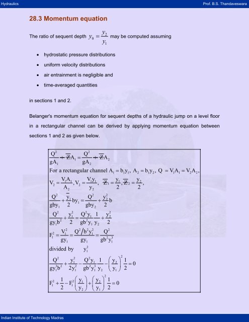
28.3 <strong>Momentum</strong> <strong>equation</strong><br />
The ratio <strong>of</strong> sequent depth<br />
<strong>Indian</strong> <strong>Institute</strong> <strong>of</strong> <strong>Technology</strong> <strong>Madras</strong><br />
y<br />
0<br />
= y<br />
y<br />
• hydrostatic pressure distributions<br />
• uniform velocity distributions<br />
• air entrainment is negligible and<br />
• time-averaged quantities<br />
in sections 1 and 2.<br />
2<br />
1<br />
may be computed assuming<br />
Belanger's momentum <strong>equation</strong> for sequent depths <strong>of</strong> a hydraulic jump on a level floor<br />
in a rectangular channel can be derived by applying momentum <strong>equation</strong> between<br />
sections 1 and 2 as given below.<br />
2 2<br />
Q Q<br />
+ ZA = + ZA<br />
gA gA<br />
1 2<br />
1 2<br />
For a rectangular channel A = b y , A = b y , Q = V A = V A ,<br />
VA Vy y y<br />
V = ,V = , Z = ,Z = ,<br />
1 1 1 1 1 2<br />
2 2<br />
1 2<br />
A2 y2 2 2<br />
Q y Q y<br />
by b<br />
gby 2 gby 2<br />
2 2 2<br />
+ 1<br />
1 = + 2<br />
1 2<br />
Q y Q y 1 y<br />
gy b 2 gb y y 2<br />
2 2 2 2<br />
+ 2<br />
1 = 2<br />
1 + 2<br />
1 1 2<br />
V Q b y Q<br />
2 2 2 2 2<br />
2<br />
1<br />
1 =<br />
gy1 =<br />
gy1 1 = 2 3<br />
gb y1<br />
F<br />
divided<br />
by y<br />
2<br />
1<br />
2 2 2<br />
Q y1 Q y1 1 ⎛y ⎞ 2 1<br />
+ − − 0<br />
3 2 2 2 3 ⎜ ⎟ =<br />
gy1b2y1 gb y1 y2 ⎝ y1 ⎠ 2<br />
2 1 2⎛ y ⎞ ⎛ 1 y ⎞ 2 1<br />
F1 + − F1 ⎜ ⎟+ ⎜ ⎟ = 0<br />
2 ⎝y2 ⎠ ⎝ y1 ⎠<br />
2<br />
2<br />
1 1 1 2 1 2 1 1 2 2<br />
2
Hydraulics Pr<strong>of</strong>. B.S. Thandaveswara<br />
<strong>Indian</strong> <strong>Institute</strong> <strong>of</strong> <strong>Technology</strong> <strong>Madras</strong><br />
2 2 2<br />
Q y1 Q y1 1 ⎛y ⎞ 2 1<br />
+ − − 0<br />
3 2 2 2 3 ⎜ ⎟ =<br />
gy1b2y1 gb y1 y2 ⎝ y1 ⎠ 2<br />
2 1 2⎛ y ⎞ ⎛ 1 y ⎞ 2 1<br />
F1 + − F1 ⎜ ⎟+ ⎜ ⎟ = 0<br />
2 ⎝y2 ⎠ ⎝ y1 ⎠ 2<br />
2 2⎛ y ⎞ ⎛ 1 y ⎞ 2<br />
2F1 + 1 −2F1 ⎜ ⎟− ⎜ ⎟ = 0<br />
⎝y2 ⎠ ⎝ y1<br />
⎠<br />
( )<br />
2 ⎛y ⎞ 2 2 ⎛ y ⎞ 2<br />
2F1 + 1 ⎜ ⎟−2F1 − ⎜ ⎟ = 0<br />
⎝ y1 ⎠ ⎝ y1<br />
⎠<br />
( )<br />
3<br />
⎛y ⎞ 2 2 ⎛y ⎞ 2 2<br />
⎜ ⎟ − ( 2F1 + 1) ⎜ ⎟+<br />
2F1 = 0<br />
⎝ y1 ⎠ ⎝ y1<br />
⎠<br />
This can be rewritten<br />
as<br />
2<br />
⎡ y2 y ⎤<br />
2 2 y2<br />
⎢ 1 ⎥<br />
y1 y1 y1<br />
⎛<br />
⎜<br />
⎢⎣⎝ ⎞<br />
⎟<br />
⎠<br />
+<br />
⎡<br />
−2F ⎢<br />
⎥⎦⎣<br />
⎤<br />
− 1⎥= 0<br />
⎦<br />
y<br />
1 0 y y uniform flow.<br />
2 ∴ − = ∴ 2 = 1<br />
y1<br />
2<br />
⎛y ⎞ 2 y2<br />
2<br />
⎜ ⎟ + − 1 =<br />
y1 y1<br />
⎝ ⎠<br />
2<br />
y211 2<br />
Hence = = 1+ 8F1 −1<br />
y12 2<br />
2<br />
2<br />
3<br />
2F 0 a quadratic <strong>equation</strong>.<br />
⎛ ⎞ − 1+ 1+ 8F<br />
⎡ ⎤<br />
⎜ ⎟<br />
⎝ ⎠<br />
⎣ ⎦<br />
y2 1 ⎡ ⎤<br />
=<br />
⎢<br />
1+ 8F<br />
2<br />
−1<br />
y ⎣<br />
1 ⎥<br />
1 2<br />
⎦<br />
2<br />
(28.1)<br />
⎛ V1<br />
⎞<br />
in which y2, y1 are sequent and initial depths respectively and F= 1 ⎜ ⎟ is the initial<br />
⎜ gy ⎟<br />
⎝ 1 ⎠<br />
Froude number. Equation 28.1 has been verified by many investigators experimentally<br />
and <strong>of</strong>ten a ratio lower than the one calculated by the <strong>equation</strong> has been recorded.<br />
Belanger , did not consider the bed shear force while deriving Eq. 28.1. Rajaratnam in
Hydraulics Pr<strong>of</strong>. B.S. Thandaveswara<br />
1965, proposed the following momentum <strong>equation</strong> taking into consideration the<br />
integrated shear force.<br />
<strong>Indian</strong> <strong>Institute</strong> <strong>of</strong> <strong>Technology</strong> <strong>Madras</strong><br />
3<br />
⎛y ⎞<br />
⎜<br />
2 y<br />
⎟ − 2 ⎡ − + ⎤<br />
⎢<br />
1 ε 2F<br />
2<br />
⎥<br />
+ 2F<br />
2<br />
=0<br />
⎜ ⎟ ⎣ ⎦<br />
⎝ y<br />
1 1<br />
1 ⎠ y1<br />
In which ε is the non dimensional integrated shear force, given by<br />
γ y<br />
2<br />
function <strong>of</strong> Froude number. Pf is the integrated shear force.<br />
P<br />
f<br />
2<br />
1<br />
(28.2)<br />
and is a<br />
He used the data <strong>of</strong> Rouse et al. , Harleman, Bakhmeteff ,Safranez , Bradley - Peterka ,<br />
along with his own. Figure 2 shows the effect <strong>of</strong> shear force on sequent depth ratio.<br />
y2<br />
___<br />
y1<br />
14<br />
12<br />
10<br />
8<br />
6<br />
4<br />
2<br />
0<br />
Eq. 28.1<br />
Eq. 28.3<br />
Eq. 28.2<br />
Belanger<br />
Rajaratnam<br />
Sarma and Newnham<br />
2 4 6 8 10<br />
Fig. 28.5 - Variation <strong>of</strong> sequent depth ratio<br />
F1
Hydraulics Pr<strong>of</strong>. B.S. Thandaveswara<br />
Sarma and Newnham 1975 introducing the momentum coefficient ( j 1.045 β = ) for the<br />
<strong>Indian</strong> <strong>Institute</strong> <strong>of</strong> <strong>Technology</strong> <strong>Madras</strong><br />
non uniform velocity distribution obtained the following modified momentum <strong>equation</strong><br />
y2 1 ⎡ ⎤<br />
=<br />
⎢<br />
1 + 10.4 F<br />
2<br />
−1<br />
y ⎣<br />
1 ⎥<br />
1 2<br />
⎦<br />
(28.3)<br />
In Eqn. 28.3, a value <strong>of</strong> β j was used by them based on the assumption <strong>of</strong> a similarity<br />
pr<strong>of</strong>ile for the velocity distribution. Eq. 28.3 gives a higher value for the sequent depth<br />
ratio, compared to the value computed from Eq.28.1. Their analysis was carried out<br />
upto a Froude number value <strong>of</strong> 4.