1. Thermo-physical properties 2. Radiation properties - nptel - Indian ...

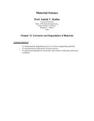
Mechanical Measurements Prof S.P.Venkatesan 

Indian Institute of Technology Madras 

Mechanical Measurements 

Module 4 

1. Thermo-physical properties 

2. Radiation properties of surfaces 

3. Gas concentration 

4. Force or Acceleration, Torque, Power 

Module 4.1 

1. Measurement of thermo-physical properties 

In engineering applications material properties are required for accurate 

prediction of their behaviour as well for design of components and systems. The 

properties we shall be interested in measuring are those that may be referred to 

generally as transport properties. The properties that we shall be interested in 

here are: 

a) Thermal conductivity 

a. Thermal conductivity 

b. Heat capacity 

c. Calorific value of fuels 

d. Viscosity



Thermal conductivity may be measured by either steady state methods or 

unsteady (transient) methods. 

(i) Steady state methods 

o Guarded hot plate method 

Solid, Liquid 

o Radial heat flow apparatus 

Liquid, Gas 

o Thermal conductivity comparator 

Solid 

Steady state methods normally involve very large measurement times since the 

system should come to the steady state, possibly starting from initial room 

temperature of all the components that make up the apparatus. Also maintaining 

the steady state requires expensive controllers and uninterrupted power and 

water supplies. 

(ii) Unsteady method 

o Laser flash apparatus 

Solid 

Even though the unsteady methods may be expensive because of stringent 

instrumentation requirements the heat losses that plague the steady sate 

methods are not present in these. The entire measurement times may be from a 

few milliseconds to seconds or at the most a few minutes. 

Thermal conductivity is defined through Fourier law of conduction. In the case of 

one-dimensional heat conduction the appropriate relation that defines the thermal 

conductivity is



q 

k =− 

∂T Q 

=− A 

∂T 

(1) 

∂x∂x In Equation 1 k is the thermal conductivity in W/m°C, q is the conduction heat flux 

in W/m 2 along the x direction given by the ratio of total heat transfer by 

conduction Q and area normal to the heat flow direction A and T represents the 

temperature. In practice Equation 1 is replaced by 

Q 

k = A 

(2) 

Δ T 

δ 

Here |ΔT| represents the absolute value of the temperature difference across a 

thickness δ of the medium. Several assumptions are made in writing the above: 

Heat conduction is one dimensional 

The temperature variation is linear along the direction of heat flow 

The above assumption presupposes that the thermal conductivity is a 

weak function of temperature or the temperature difference is very 

small compared to the mean temperature of the medium 

With this background, the following general principles may be enunciated, that 

are common to all methods of measurement of thermal conductivity: 

Achieve one dimensional temperature field within the medium 

Measure heat flux 

Measure temperature gradient 

Estimate thermal conductivity 

In case of liquids and gases suppress convection 

Parasitic losses are reduced/ eliminated/estimated and 

are accounted for – in all cases



(i) Steady state methods 

Guarded hot plate apparatus: solid sample 

The guarded hot plate apparatus is considered as the primary method of 

measurement of thermal conductivity of solid materials that are available in the 

form of a slab (or plate or blanket forms). The principle of the guard has already 

been dealt with in the case of heat flux measurement in Module 3. It is a method 

of reducing or eliminating heat flow in an unwanted direction and making it take 

place in the desired direction. At once it will be seen that one-dimensional 

temperature field in the material may be set up using this approach in a slab of 

material of a specified area and thickness. Schematic of a guarded hot plate 

apparatus is shown in Figure 1. Two samples of identical size are arranged 

symmetrically on the two sides of an assembly consisting of main and guard 

heaters. The two heaters are energized by independent power supplies with 

suitable controllers. Heat transfer from the lateral edges of the sample is 

prevented by the guard backed by a thick layer of insulation all along the 

periphery. The two faces of each of the samples are maintained at different 

temperatures by heaters on one side and the cooling water circulation on the 

other side. However identical one-dimensional temperature fields are set up in 

the two samples.



Insulation 

Cold 

Water IN 

G = 

Sample 

Sample 

Cold 

Water OUT 

Insulation 

Cold 

Cold 

Water IN Water OUT 

L=25 

Main Heater 

Guard Heater 

Figure 1 Guarded hot plate apparatus schematic 

Guard Heater 

50 mm wide 

Thermocouple 

junction 

2 mm gap 

All round 

Main Heater 

200x200 mm 

Figure 2 Detail of the main and guard heaters showing 

the thermocouple positions 

The details of the main and guard heaters along with the various thermocouples 

that are used for the measurement and control of the temperatures are shown in 

the plan view shown in Figure 2. As usual there is a narrow gap of 1 – 2 mm all 

round the main heater across which the temperature difference is measured and 

maintained at zero by controlling the main and guard heater inputs. However the 

sample is monolithic having a surface area the same as the main, guard and gap 

all put together. Temperatures are averaged using several thermocouples that 

are fixed on the heater plate and the water cooled plates on the two sides of the 

samples. The thermal conductivity is then estimated based on Equation 2, where



the heat transfer across any one of the samples is half that supplied to the main 

heater and the area is the face area of one of the samples. 

Typically the sample, in the case of low conductivity materials, is 25 mm thick 

and the area occupied by the main heater is 200×200 mm. The heat input is 

adjusted such that the temperature drop across the sample is of the order of 5°C. 

In order to improve the contact between heater surface and the sample surface a 

film of high conductivity material may be applied between the two. Many a time 

an axial force is also applied using a suitable arrangement so that the contact 

between surfaces is thermally good.



Example 1 

A guarded hot plate apparatus is used to measure the thermal 

conductivity of an insulating material. The specimen thickness is 25 ± 

0.5 mm. The heat flux is measured within 1% and is nominally 80 W/m 2 . 

The temperature drop across the specimen under the steady state is 5 ± 

0.2°C. Determine the thermal conductivity of the sample along with its 

uncertainty. 

The given data is written down as (all are nominal values) 

2 

q = 80 W / m , Δ T = 5 ° C, δ = 25 mm= 0.025 m 

Using Equation 2, the nominal value of the thermal conductivity is 

qδ 

80× 0.025 

k = = = 0.4 W / m° C 

ΔT 

5 

The uncertainties in the measured quantities specified in the problem are 

q 80 

2 

δq =± =± =± 0.8 W / m , δ ( Δ T) =± 0.2 ° C, 

100 100 

δδ =± 0.5 mm =± 0.0005 m 

Logarithmic differentiation is possible and the error in the thermal 

conductivity estimate may be written down as



( ) 2 

ΔT 

2 2 

⎛δq⎞ ⎛δ⎞ ⎛δδ ⎞ 

Δ k =± k ⎜ ⎟ + ⎜ ⎟ + ⎜ ⎟ 

⎝ q ⎠ ⎝ ΔT ⎠ ⎝ δ ⎠ 

2 2 2 

⎛0.8 ⎞ ⎛0.2 ⎞ ⎛0.0005 ⎞ 

=± 0.4× ⎜ ⎟ + ⎜ ⎟ + ⎜ ⎟ =± 0.018 W / m° C 

⎝ 80 ⎠ ⎝ 5 ⎠ ⎝ 0.025 ⎠ 

Thus the thermal conductivity is estimated within an error margin of 

0.018 

± × 100 ≈± 4.6% . 

0.4



Guarded hot plate apparatus: liquid sample 

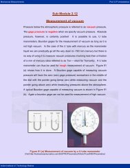
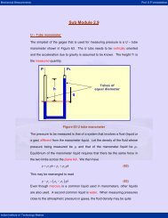
Measurement of thermal conductivity of liquids (and gases) is difficult because it 

is necessary to make sure that the liquid is stationary. In the presence of 

temperature variations and in the presence of gravity the liquid will start moving 

around due to natural convection. There are two ways of immobilizing the fluid: 

a) Use a thin layer of the fluid in the direction of temperature gradient so that the 

Grashof number is very small and the regime is conduction dominant b) Set up 

the temperature field in the fluid such that the hot part is above the cold part and 

hence the layer is in the stable configuration. The guarded hot plate apparatus is 

suitably modified to achieve these two conditions. 

Gallery in 

which 

excess 

liquid 

collects 

Main Heater 

Cold 

Water IN 

Cold 

Water IN 

Guard Heater 

Cold 

Water OUT 

Cold 

Water OUT 

Liquid layer 

Figure 3 Guarded hot plate apparatus for the measurement 

of thermal conductivity of liquids 

Figure 3 shows schematically how the conductivity of a liquid is measured using 

a guarded hot plate apparatus. The symmetric sample arrangement in the case 

of a solid is replaced by a single layer of liquid sample with a guard heater on the 

top side. Heat flow across the liquid layer is downward and hence the liquid layer 

g 

Insulation



is in a stable configuration. The thickness of the layer is chosen to be very small 

(of the order of a mm) so that heat transfer is conduction dominant. The guard 

heat input is so adjusted that there is no temperature difference across the gap 

between the main and the guard heaters. It is evident that all the heat input to 

the main heater flows downwards through the liquid layer and is removed by the 

cooling arrangement. Similarly the heat supplied to the guard heater is removed 

by the cooling arrangement at the top. 

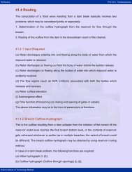
Radial heat conduction apparatus for liquids and gases: 

Another apparatus suitable for the measurement of thermal conductivity of fluids 

(liquids and gases) is one that uses radial flow of heat through a very thin layer of 

liquid or gas. A cross sectional view of such an apparatus is shown in Figure 4. 

Heater is in the form of a cylinder (referred to as bayonet heater or the plug) and 

is surrounded by a narrow radial gap that is charged with the liquid or the gas 

whose thermal conductivity is to be measured. The outer cylinder is actually a 

jacketed cylinder that is cooled by passing cold water. Heat loss from the 

bayonet heater except through the annular fluid filled gap is minimized by the use 

of proper materials. Thermocouples are arranged to measure the temperature 

across the fluid layer. Since the gap (the thickness of the fluid layer) is very 

small compared to the diameter of the heater heat conduction across the gap 

may be very closely approximated by that across a slab. Hence Equation 2 may 

be used in this case also.



Sample 

fluid 


Cooling water in 

Gap δ 

Cooling water out 


Heater 

D 

Sample 

fluid 

Figure 4 Radial heat flow apparatus for liquids and gases 

Typical specifications of an apparatus of this type are given below: 

Diameter of cartridge heater D = 37 mm 

Radial clearance = 0.3 mm 

Heat flow area A = 0.0133 m 2 

Temperature difference across the gap ΔT ~ 5°C 

Heater input Q = 20 – 30 W 

The diameter is about 75 times the layer thickness. The use of this apparatus 

requires a calibration experiment using a fluid of known thermal conductivity 

(usually dry air) filling the gap. Thermal conductivity of air is well known (as a 

function of temperature) and is available as tabulated data. If an experiment is 

conducted with dry air, heat transferred across the gap may be determined using 

Fourier law of heat conduction. The heat input to the bayonet heater is 

measured and the difference between these two should represent the heat loss. 

The experiment may be conducted with different amounts of heat input (and 

hence different temperature difference across the air layer) and the heat loss 

estimated. This may be represented as a function of the temperature difference



across the gap. When another fluid is in the annular gap, the heat loss will still 

be given by the previously measured values. Hence the heat loss may be 

deducted from the heat input to get the actual heat transfer across the fluid layer. 

At once Equation 2 will give us the thermal conductivity of the fluid. 

Heat loss data has been measured in an apparatus of this kind and is shown as 

a plot in Figure 5. The data shows mild nonlinear behavior. Hence the heat loss 

may be represented as a polynomial function of the temperature difference 

across the gap using regression analysis. The heat loss is a function of 

θ = TP −TJand is given by the polynomial 

2 3 

L = 0.0511+ 0.206θ + 0.0118θ − 0.000153θ 

(3) 

In the above TP is the plug temperature and TJ is the jacket temperature. 

Loss, W 

3.5 

3 

2.5 

2 

1.5 

1 

0.5 

0 

0.5 2.5 4.5 6.5 8.5 

Temperature Difference, o C 

Figure 5 Heat loss calibration data for a radial flow 

thermal conductivity apparatus



Example 2 

A radial heat flow apparatus has the following specifications: 

Gap δ = 0.3 mm. Heat flow area A = 0.0133 m 2 

The following data corresponds to an experiment performed with unused 

engine oil (SAE 40): 

Heater voltage: V = 40 Volts, Heater resistance: R = 53.5 Ω 

Plug temperature: TP = 32.9°C, Jacket temperature: TJ = 28.2°C 

What is the thermal conductivity of the oil sample? If the measured 

parameters have the following uncertainties what will be the uncertainty 

in the estimated value of the thermal conductivity? 

ΔV = ± 0.5 V, ΔT = ± 0.2°C 

The heat loss is a function of θ = TP −TJand is given by the polynomial 

2 3 

L = 0.0511+ 0.206θ + 0.0118θ − 0.000153θ 

The heat loss itself is estimated by the above formula with an error bar of 

± 0.5%. 

First we determine the nominal value of the thermal conductivity using 

the nominal values of all the measured quantities. 

The electrical heat input to the heaters is given by 

2 2 

V 40 

Qe= = = 29.91 W 

R 53.5 

The temperature drop across the sample liquid is 

θ = T − T = 32.9 − 28.2 = 4.7° 

C 

P J 

The heat loss may at once be calculated as 

2 3 

L= 0.0511+ 0.206× 4.7 + 0.0118× 4.7 − 0.000153× 4.7 = 

1.26 W



(This agrees with the value shown in Figure 5) 

The heat conducted across the liquid layer is then given by 

Q = Q − L= 29.91− 1.26 = 28.65 W 

c e 

Using Equation 2 the nominal value of the thermal conductivity of oil 

sample is 

−3 

Qc 

δ 28.65× 0.3× 10 

k = = = 0.138 W / m° C 

A θ 0.0133× 4.7 

Now we calculate the uncertainty in the nominal value of the thermal 

conductivity estimated above. Only the heat transferred and the 

temperatures are susceptible to error. We know 

2 

V 

thatQc 

= Qe − L= − L. 

Assuming that R is not susceptible to any 

R 

∂ Qc 2V2× 40 ∂Qc 

error, we have = = = 1.495 W / V , = −1. 

Hence the 

∂V 

R 53.5 

∂L 

error in the measured value of the heat conducted across the liquid layer 

is 

2 2 

c c 

⎛∂Q ⎞ ⎛∂Q ⎞ 

δQc=± 

⎜ Δ V + ΔL 

∂V ⎟ ⎜ 

∂L 

⎟ 

⎝ ⎠ ⎝ ⎠ 

( ) ( ) 

2 2 

=± 1.495× 0.5 + − 1× 0.05× 1.26 =± 0.75 W 

The errors in the measured temperatures are equal and hence the error 

in the measured temperature difference is 

δθ =± 2Δ T =± 2 × 0.2 =± 0.283° 

C. 

The error propagation formula gives



⎝ c ⎠ 

2 2 

⎛δQc⎞ ⎛δθ ⎞ 

δ k =± k ⎜ ⎟ + ⎜ ⎟ 

Q ⎝ θ ⎠ 

2 2 

⎛ 0.75 ⎞ ⎛0.28 ⎞ 

=± 0.138× ⎜ ⎟ + ⎜ ⎟ =± 0.066 W / m° C 

⎝28.65 ⎠ ⎝ 4.7 ⎠ 

Thus the measured value of thermal conductivity of oil sample is 0.138 ± 

0.066 W/m°C. 

Thermal conductivity comparator 

Thermal conductivity comparator is a method in which the thermal conductivity of 

a sample is obtained by comparison with another sample of known thermal 

conductivity. This method is especially useful for the determination of thermal 

conductivity of good conductors, such as metals and alloys. The principle of the 

method may be explained with reference to Figure 6. 

A: Standard 

reference 

material (SRM) 

B: Material of 

unknown 

thermal 

conductivity 

Hot 

Cold 

Insulation 


junctions 

Figure 6 Schematic of a thermal conductivity comparator 

A sample of standard reference material (SRM - a material whose thermal 

conductivity is known and guaranteed by the manufacturer) is placed in series 

with the material whose thermal conductivity needs to be estimated. Both the 

materials have identical cross section (usually cylindrical) and heat is allowed to 

LA 

LB



flow, under the steady state, as indicated in the figure. Thermocouples are 

arranged as shown in order to estimate the temperature gradients in each 

material. Heat loss in the lateral direction is prevented by the provision of 

insulation as shown. With the nomenclature of Figure 6, we have the following: 

k ΔT k ΔT L ΔT 

A A B B B A 

= or kB = kA 

LALB LA ΔTB 

The above expression is based on the fact that the conduction heat fluxes 

through the sample and the SRM are the same. The lengths and temperature 

differences are the measured quantities and k A is the known thermal conductivity 

of the SRM. 

(4)



Example 3 

A thermal conductivity comparator uses a standard reference material 

(SRM) of thermal conductivity 45 ± 2% W/m-K. Two thermocouples 

placed 22 ± 0.25 mm apart indicate a temperature difference of 2.5 ± 

0.2°C. The material of unknown thermal conductivity is in series with the 

SRM and indicates a temperature difference of 7.3±0.2°C across a 

length of 20 ± 0.25 mm. Determine the thermal conductivity of the 

sample and its uncertainty. 

The given data may be written down using the nomenclature of Figure 6. 

k = 45 W / m° C, Δ T = 2.5 ° C, Δ T = 7.3 ° C, L = 22 mm, L = 20 mm 

A A B A B 

The nominal value of the thermal conductivity of the sample is then 

given by 

LB ΔTA 

20 2.5 

kB = kA = 45× × = 14 W / m° C 

L ΔT 

22 7.3 

A B 

The uncertainties specified are 

0.25 0.25 

δkA =± 2%, δLA =± × 100 = 1.14%, δLB 

=± × 100 = 1.25%, 

22 20 

0.2 0.2 

δΔ TA =± × 100 = 8%, δΔ 

TB 

=± × 100 = 

2.74% 

2.5 7.3



Since the unknown thermal conductivity depends on the other 

quantities involving only products of ratios, the percentage error may 

be directly calculated using percent errors in each of the measured 

quantities. Thus 

( ) ( ) ( ) ( ) ( ) 

2 2 2 2 2 

B =± A + A + B + A + B 

δk δk δL δL δT δT 

( ) ( ) ( ) ( ) ( ) 

2 2 2 2 2 

=± 2 + 1.14 + 1.25 + 8 + 2.74 =± 8.85% 

The uncertainty in the thermal conductivity is thus equal to 

(ii) Unsteady method 

8.85 

δ kB= ± 14× =± 1.24 W / m° C . 

100 

Though many methods are available under the unsteady category only one of 

them, viz. the laser flash method, will be considered as a representative one. 

Also it is the most commonly used method in laboratory practice and laser flash 

apparatus are available commercially, though very expensive. 

The laser flash method imposes a pulse of heat to a thin sample and monitors 

the back surface temperature as a function of time. The schematic of the laser 

flash apparatus is shown in Figure 7.



Figure 7 Schematic of the laser flash apparatus 

The sample is in the form of a thin slab and is maintained at the desired 

temperature by placing it in a furnace. The front face of the slab is heated with a 

laser or flash pulse and the temperature of the back face is monitored as a 

function of time. The laser or flash pulse is of such intensity that the temperature 

will rise by only a few degrees. In other words the temperature rise is very small 

in comparison with the mean temperature of the sample. If the thermal diffusivity 

of the material of the sample is α, the non-dimensional time is defined as 

αt 

Fo = . The non-dimensional temperature is defined as 

2 

L 

T 

θ = where Tmax is 

Tmax 

the maximum temperature reached by the back surface of the sample. The 

following plot (Figure 8) shows the shape of the response using the non- 

dimensional coordinates. Note that it is not necessary to know the temperatures 

in absolute terms since only the ratio is involved. It is found that the response is 

0.5 at a non-dimensional time is 1.37 as indicated in the figure. The quantity that 

is estimated from the measurement is, in fact, the thermal diffusivity of the 

material. Thus if t1/2 is the time at which the response is 0.5, we have 

2 

1.37 L 

α = (5) 

t 

1/2 

Laser or 

Flash 

Sample 

Furnace, Tf 

A 

m 

pl 

ifi 

er 

Recorder 

Sample thickness L 

Sample material thermal diffusivity α



If the density ρ and specific heat capacity c of the material are known (they may 

be measured by other methods, as we shall see later) the thermal conductivity is 

obtained as 

k = ρcα (6) 

In practice the temperature signal is amplified and manipulated by computer 

software to directly give the estimate of the thermal diffusivity of the solid sample. 

Non-dimensional temperature 

0.8 

0.6 

0.4 

0.2 

b) Measurement of heat capacity 

1 

0 

1.37, 0.5 

0 1 2 3 4 

Non-dimensional time 

Figure 8 Response at the back surface 

Heat capacity is an important thermo-physical property that is routinely measured 

in the laboratory. In material characterization heat capacity is one of the 

important properties whose changes with temperature indicate changes in the 

material itself. The method used for measurement of heat capacity is usually a 

calorimetric method, where energy balance in a controlled experiment gives a 

measure of the heat capacity. 

Heat capacity of a solid:



We consider first the measurement of heat capacity of a solid material. The 

basic principle of the calorimetric method is the application of the first law of 

thermodynamics (heat balance) in a carefully conducted experiment. A weighed 

sample of solid material, in granular or powder form, whose heat capacity is to be 

measured is heated prior to being transferred quickly into a known mass of water 

or oil (depending on the temperature level) contained in a jacketed vessel. Let 

the mass of the solid be m and let it be at a temperature T3 before it is dropped 

into the calorimeter. Let T1 be the initial temperature of the calorimeter and the 

jacket. Let the mass specific heat product of the calorimeter, stirrer and the liquid 

in the calorimeter be C. Let T2 be the maximum temperature reached by the 

calorimeter with its contents including the mass dropped in it. Let c be the 

specific heat of the solid sample that is being estimated using the experimental 

data. We recognize that there is some heat loss that would have taken place 

over a period of time at the end of which the temperature has reached T2. Let 

the heat loss be QL. 

Precision 

thermometer 

Thermometer 

Calorimeter 

Containing 

containing 

water Water or oil Oil 

Figure 9 Calorimeter for the measurement of specific heat of a solid 

Energy balance requires that 

Drop 

Hot 

Mass 

Stirrer 



Water 

Jacket at 

Constant 

temperature 

Temperature



( ) ( ) 

C T − T + Q = mc T − T 

(7) 

2 1 L 3 2 

Now let us look at how we estimate the heat loss. For this we show the typical 

temperature-time plot that is obtained in such an experiment. 

Figure 10 Typical temperature time trace 

If there were to be no loss the temperature-time trace should be like that shown 

by the purple trace made up of two straight lines. After the temperature reaches 

' 

T 2 it should remain at that value! However there is heat loss and the 

temperature-time trace is a curve that follows the blue line. After the temperature 

reaches a maximum value of T2 it decreases with time. The rate of decrease is, 

in fact, an indication of how large the heat loss is. If we assume that temperature 

rise of the calorimeter is very small during the mixing part of the experiment, we 

may assume the rate of heat loss to be linear function of temperature difference 

. Now consider the state of affairs after the maximum 

given by Q = K( T −T 

) 

L 

1 

temperature has been passed. The calorimeter may be assumed to be a first 

order system with 

Temperature, o C 

25 

24 

23 

22 

21 

20 

With heat loss No heat loss 

M 

I 

X 

MIXING 

I T’2 

N T2 

G 

T1 

COOLING 

0 10 20 30 40 50 

Time, s 

dT 

C + K( T − T1) 

= 0 

(8) 

dt



Here we assume that K is the same as the K in the heating part (mixing part) of 

the experiment. If we approximate the derivative by finite differences, we may 

recast Equation 8 as 

⎛ΔT⎞ ⎜ ⎟ 

Δt 

K = C 

⎝ ⎠ 

T T 

( − ) 

1 

The numerator on the right hand side of Equation 9 is obtained by taking the 

slope of the cooling part of the curve at any chosen t after the cooling has started 

and thus at the corresponding temperature. Now we look at the heat loss term. 

The heat loss in the mixing part of the experiment may be obtained by integrating 

the rate of heat loss with respect to time between t = 0 and the time tmax at which 

the maximum temperature is reached. In fact the temperature time curve may be 

approximated by a triangle and hence the heat loss is 

L 

( T −T 

) 

tmax 

2 1 

∫ ( 1) max 

(10) 

2 

0 

Q = K T −T dt ≈ K t 

This is substituted in Equation 7 and rearranged to get 

( 2 − 1) 

+ 

( ) 

( − ) 

K T T t 

C T T Q 

C( T2 − T1) 

+ 

L 

c = = 

2 

mT−TmT−T ( ) 

3 2 3 2 

2 1 max 

(9) 

(11)



Example 4 

In a calorimeter experiment for determination of specific heat of glass 

beads, 0.15 kg of beads at 80°C are dropped in to a calorimeter 

which is equivalent to 0.5 kg of water, at an initial temperature of 

20°C. The maximum temperature of 22.7°C of the mixture occurs by 

linear increase of the temperature in 10 s after the mixing starts. The 

subsequent cooling shows that the temperature drops at 0.2°C/min 

when the temperature is 22.7°C. Estimate the specific heat of glass 

beads. Assume that the specific heat of water is 4.186 kJ/kg°C. 

The given data is written down using the nomenclature introduced in 

the text: 

m= 0.015 kg, T = 20 ° C, T = 22.7° 

C 

3 

1 2 

T = 80 ° C, C = 0.5× 4.186 = 2.093 kJ / ° C 

ΔT 

0.2 

tmax = 10 s, = 0.2 ° C/ min = = 0.0033 ° C/ s 

Δt 

60 

The cooling constant may be calculated as 

ΔT 

C 

t 2.093× 0.0033 

K = Δ = = 0.0026 kW / ° C 

( T −T ) ( 22.7 −20) 

2 1 

The heat loss during the mixing process is then approximated as 

( T T ) t 

( ) 

2 − 1 max 22.7 − 20 × 10 

QL≈ K = 0.0026× = 0.035 kW 

2 2 

The specific heat of glass bead sample may now be estimated as 

( ) 

mT ( T) 

3 2 

( ) 

( ) 

C T2 − T1 + QL 

2.09× 22.7 − 201 + 0.035 

c= = = 0.661 kJ / kg° C 

− 0.15× 80 −22.7



Heat capacity of liquids 

Essentially the same calorimeter that was used in the case of solid samples may 

be used for the measurement of specific heat of liquids, with the modifications 

shown in Figure 11. The sample liquid is taken in the calorimeter vessel and 

allowed to equilibrate with the temperature of the constant temperature fluid in 

the jacket and the rest of the works. The heater is energized for a specific time 

so that a measured amount of thermal energy is added to the sample liquid. 

Stirrer (not shown) will help the liquid sample to be at a uniform temperature. 

The temperature increase of the liquid at the end of the heating period is noted 

down. The liquid specific heat is then estimated using energy balance. Effect of 

heat loss may be taken into account by essentially the same procedure that was 

used in the earlier case. 

1 

5 

9 

4 

3 

Figure 11 Apparatus for measurement of specific heat of liquids 

(1 – Lagging, 2 – Constant temperature bath, 3- Heater, 4 – Sample liquid, 5 

– Precision thermometer, 6 – Energy meter, 7 – Switch, 8 – Power supply, 9 

– Insulating lid) 

2 

6 

7 

8



c) Measurement of calorific value of fuels 

Calorific or heating value of a fuel is one of the most important properties of a 

fuel that needs to be measured before the fuel can be considered for a specific 

application. The fuel may be in the liquid, gaseous or solid form. The 

measurement of heating value is normally by calorimetry. While a continuous 

flow calorimeter is useful for the measurement of heating values of liquid and 

gaseous fuels, a bomb calorimeter is used for the measurement of heating value 

of a solid fuel. 

Preliminaries: 

Heating value of a fuel or more precisely, the standard enthalpy of combustion 

is defined as the enthalpy change 

0 

T 

Δ H that accompanies a process in which the 

given substance (the fuel) undergoes a reaction with oxygen gas to form 

combustion products, all reactants and products being in their respective 

standard states at T = 298.15K = 25° C . A bomb calorimeter (to be described 

later) is used to determine the standard enthalpy of combustion. The process 

that takes place is a t a constant volume. Hence the process that occurs in a 

calorimeter experiment for the determination of the standard enthalpy of 

combustion is process I in Figure 12. What is desired is the process shown as III 

in the figure. We shall see how to get the information for process III from that 

measured using process I.



Figure 12 Processes in a calorimeter experiment 

Let the calorimeter have a heat capacity equal to C. The change in the internal 

energy of the calorimeter when the temperature changes from T1 to T2 

T2 is ∫ 

T1 CdTassuming 

that C is independent of pressure. If we neglect work 

interaction due to stirring, I law applied to a perfectly insulated calorimeter (Q = 0) 

shows that Δ UI= 0 during process I. In the process shown as II the products and 

the calorimeter are at temperature T1. Thus, for process II we should 

T 2 

have Δ U =ΔU −∫ CdT. 

Thus it is clear that Δ U =Δ U =− CdT=ΔU II I 

Reactants at 

pressure p1 and 

temperature T1 

T 1 

T2 II T1 ∫ 

T1 0 

T1 

. The 

last part results by noting that the internal energy is assumed to be independent 

0 0 

of pressure. Note that by definition H U ( PV) 

Δ =Δ +Δ . Since the products are 

T1 T1 

in the gaseous state, assuming the products to have ideal gas behavior, we 

have, ( ) ( ) 

Δ pV = p V − p V = n −nℜTwhere the n2 represents the number of 

2 2 1 1 2 1 1 

Products at 



Products at 



Products at 



moles of the product and n1 the number of moles of the reactant andℜ is the 

I 

II 

III



universal gas constant. Thus it is possible to get the desired heat of combustion 

as 

( ) 

0 

T12 1 g 

T 2 

Δ H = n −n R T−∫ CdT 

(12) 

T 1 

In a typical experiment the temperature change is limited to a few degrees and 

hence the specific heat may be assumed to be a constant. Under this 

assumption Equation 12 may be replaced by 

( ) ( ) 

0 

T12 1 g 2 1 

Δ H = n −n R T−C T − T 

(13) 

The Bomb calorimeter: 

1 

2 

7 

6 

5 

3 

4 

1.Stirrer 

2.Calorimeter bomb 

3.Jacket 

4.Calorimeter vessel 

5.PRT 

6.Ignition lead 

7.Jacket lid 

From: www.fire-testing.com 

Figure 13 Bomb calorimeter schematic 

Schematic of a bomb calorimeter used for the determination of heating value 

(standard enthalpy of combustion) of a solid fuel is shown in Figure 13. The 

bomb is a heavy walled pressure vessel within which the combustion reaction will 

take place at constant volume. At the bottom of the bomb is placed sufficient



amount of water such that the atmosphere within the bomb remains saturated 

with water vapor throughout the experiment. This guarantees that the water that 

may be formed during the combustion reaction will remain in the liquid state. The 

bomb is immersed within a can of water fitted with a precision thermometer 

capable of a resolution of 0.01°C. This assembly is placed within an outer water 

filled jacket. The jacket water temperature remains the same both before and 

after the combustion within the bomb. There is no heat gain or loss to the bomb 

from outside and the process may be considered to be adiabatic. The fuel is 

taken in the form of a pellet (about 1 g) and the combustion is accomplished by 

initiating it by an electrically heated fuse wire in contact with the pellet. The 

bomb is filled with oxygen under high pressure (25 atmospheres) such that there 

is more than enough oxygen to guarantee complete combustion. The heating 

value is estimated after accounting for the heat generated by the fuse wire 

consumed to initiate combustion. 

Benzoic acid (C7H6O2 - solid) is used as a standard reference material of known 

0 

heat of reaction Δ H =− 3227 kJ / mol . Benzoic acid is taken in the form of a pellet 

and burnt in a bomb calorimeter to provide the data regarding the heat capacity 

of calorimeter. A typical example is given below.



Example 5 

A pellet of benzoic acid weighing 0.103 g is burnt in a bomb calorimeter and the 

temperature of the calorimeter increases by 2.17°C. What is the heat capacity of 

the calorimeter? 

Consider the combustion reaction. 7.5 moles of oxygen are required for 

complete combustion of benzoic acid. 

CHO + 7.5O→ 7CO+ 3HO 

 

7 6 2 2 2 2 

Solid Gas Gas Liquid 

The change in the number of moles during the reaction is given by 

Δ n = n2 − n1 = 7 

 

− 7.5 

 

=−0.5 

CO2 in O2 in 

the product t he reac tan t 

Per mole of benzoic acid basis, we have 

Δ U=ΔH−ΔnℜT =−3227 −( − 0.5) × 8.3143× 298 

=−3225.8 

kJ / mol 

The molecular weight of benzoic acid is calculated as 

Molecular weight = 12.011× 7 

 

+ 1.008× 6 

 

+ 15.9995× 2 

C H2 

O 

= 122.12 g / mol 

0.103 

0.000843 mol 

Thus 0.103 g of benzoic acid corresponds to 122.12 = 

. The heat 

released by combustion of this is 

Q = 0.000843× 3225.8 = 

2.7207 kJ



The temperature increase of the calorimeter has been specified as ΔT = 2.17°C. 

Hence the heat capacity of the calorimeter is 

Q 2.7207 

C = = = 1.2538 kJ / ° C 

Δ T 2.17 


25 

24.5 

24 

23.5 

23 

22.5 

22 

21.5 

ΔT 

0 4 8 

Time, min 

12 16 

Figure 14 Bomb calorimeter data for example 6



Example 6 

In a subsequent experiment, the calorimeter of Example 5 is used to determine 

the heating value of sugar. A pellet of sugar weighing 0.303 g is burnt and the 

corresponding temperature rise indicated by the calorimeter is 3.99°C. What is 

the heat of combustion of sugar? 

Figure 14 shows the variation of temperature of the calorimeter during the 

experiment. Since heat losses are unavoidable the temperature will start 

reducing as shown in the figure. By using ΔT as shown in the figure the effect of 

the heat losses may be accounted for. Note that the work due to stirrer may itself 

compensate for the heat loss to some extent. The slope of the cooling curve 

takes this into account naturally. 

Molecular formula for sugar is C12H22O11. The molecular weight of sugar is found 

as 

Molecular weight = 12.011× 12 + 1.008× 22 + 

15.9995× 11 

= 342.3 g / mol 

C H2 

The mass of sugar pellet of 0.303 g corresponds to 

The heat release in the calorimeter is calculated based on 

C = 1.2538 kJ / ° C 

as 

Q =−CΔ T =− 1.2538× 3.99 =−5.003 

kJ 

The combustion reaction for sugar is given by 

O 

0.303 

0.000885 mol 

342.3 = 

T 3.99 C 

Δ = ° and



C H O + 12O → 12CO + 11H O 

12 22 11 2 2 2 

 

Solid Gas Gas Liquid 

Hence there is no change in the number of moles before and after the reaction. 

Thus the heat of reaction is no different from the heat released and thus 

0 5.003 

Δ H =− = 5651.9 kJ / mol 

0.000885 

The next case we consider is the measurement of heating value of a gaseous 

fuel. 

Continuous flow calorimeter: 


Water 

IN 

Well insulated enclosure 

Venturi 


Water 

OUT 

Rotameter 


Gas IN 

Figure 15 Schematic of a continuous flow calorimeter 

Figure 15 shows the schematic of a continuous flow calorimeter used for the 

determination of heating value of a gaseous fuel. We assume that all the 

processes that take place on the gas side are at a mean pressure equal to the 

atmospheric pressure. The gas inlet pressure may be just “a few mm of water 

column gage” and hence this assumption is a good one. As the name indicates, 

the processes that take place in the calorimeter are in the steady state with



continuous flow of the gas air mixture (air provides oxygen for combustion) and 

the coolant (water) through the cooling coils. As indicated temperatures and flow 

rates are measured using appropriate devices familiar to us from Module 2. The 

gas air mixture is burnt as it issues through a nozzle that is surrounded by a 

cooling coil through which a continuous flow of cooling water is maintained. The 

enthalpy fluxes involved in the apparatus are given below: 

1) Gas air mixture (mg) entering in at room temperature (Tg,entry) 

Mass flow measured using venturi 

Temperature measured using a liquid in glass thermometer 

2) Products of combustion leaving at a higher temperature (Tg,exit) 


3) Cooling water (mw)entering at constant temperature (Tw,entry) 

Mass flow measured by rotameter 

4) Cooling water stream leaves at a higher temperature (Tw,exit) 


Energy balance requires that the following hold: 

( ) 

mHV= C T − C T + m C T − T 

(14) 

g pp g,exit pm g,entry w pw w,exit w,entry 

In the above equation HV is the heating value of the fuel, Cpp is the specific heat 

of products of combustion and Cpm is the specific heat of gas air mixture. The 

determination of Cpp will certainly require knowledge of the composition of the 

products formed during the combustion process. The products of combustion 

have to be obtained by methods that we shall describe later. In the case of



hydrocarbon fuels with complete combustion (possible with enough excess air) 

the products will be carbon dioxide and water vapor. If the exit temperature of 

the products is above 100°C the water will be in the form of steam or water 

vapor. The estimated heating value is referred to as the lower heating value 

(LHV) as opposed to the higher heating value (HHV) that is obtained if the water 

vapor is made to condense by recovering its latent heat. 

d) Measurement of viscosity of fluids 

Viscosity of a fluid is a thermo-physical property that plays a vital role in fluid flow 

and heat transfer problems. Viscosity relates the shear stress within a flowing 

fluid to the spatial derivative of the velocity. A Newtonian fluid follows the relation 

du 

τ=μ (15) 

dy 

In the above is the shear stress in Pa, u is the fluid velocity in m/s, y is the 

coordinate measured as indicated in Figure 16 and is the dynamic viscosity of 

the fluid in Pa s or kg/m s. Viscosity is also referred in terms of Poise which is 

equal to 0.1 kg/m s. The ratio of dynamic viscosity to the density of the fluid 

is called the kinematic viscosity . The unit of is m 2 /s. An alternate unit is the 

Stoke that is equal to 0.0001 m 2 /s. 

y 

u du 

is the slope of this line 

dy 

Figure 16 Newton law of viscosity explained



The shear stress introduced through Equation 15 accounts for the slowing down 

of a higher velocity layer adjacent to a lower velocity layer. It also accounts for 

the frictional drag experienced by a body past which a fluid is flowing. 

Measurement of viscosity thus is based on the measurement of any one of these 

effects. 

Three methods of measuring viscosity of a fluid are discussed here. These are 

based on: 

i. Laminar flow in a capillary: The pressure drop in the fully developed part 

of the flow is related to the wall shear that is related in turn to viscosity. 

ii. Saybolt viscometer: The time taken to drain a standard volume of liquid 

through a standard orifice is related to the viscosity. 

iii. Rotating cylinder viscometer: The torque required to maintain rotation of a 

drum in contact with the liquid is used as a measure of viscosity. 

i) Laminar flow in a capillary: 

Velocity profile 

Developing u = u(x,r) 

Circular tube of 

diameter D 

x = 0 x= L dev 

Velocity profile 

Developed u = u(r) 

r 

x 

L dev = 0.05×D×Re D 

Figure 17 Laminar flow of a fluid in a circular tube



The nature of flow in a straight circular tube is shown in Figure 17. The fluid 

enters the tube with a uniform velocity. If the Reynolds number is less than 

about 2000 the flow in the tube is laminar. Because of viscous forces within the 

fluid and the fact that the fluid satisfies the no slip condition at the wall, the fluid 

velocity undergoes a change as it moves along the tube, as indicated in the 

figure. At the end of the so called developing region the fluid velocity profile 

across the tube has an invariant shape given by a parabolic distribution of u with 

y. This region is referred to as the fully developed region. The axial pressure 

gradient is constant in this part of the flow and is related to the fluid viscosity and 

the flow velocity. The requisite background is available to you from your course 

on Fluid Mechanics. We make use of the results of Hagen Poiseuille flow. You 

may recall that this was used earlier while discussing the transient behavior of 

pressure sensors. 

Over 

Flow 

Pump 

Constant 

Head Tank 

Manometer 

Rotameter 

Figure 18 Laminar flow in a capillary and viscosity measurement 

A schematic of the apparatus used for the measurement of viscosity of a liquid is 

shown in Figure 18. The apparatus consists of a long tube of small diameter 

L e 

L 

h 

Capillary 

Tube



(capillary) in which a steady flow is established. By connecting the capillary to a 

constant head tank on its upstream the pressure of the liquid is maintained 

steady at entry to the capillary. The pump – overflow arrangement maintains the 

level of the liquid steady in the constant head tank. The mean flow velocity is 

measured using a suitable rotameter just upstream of the capillary. The pressure 

drop across a length L of the capillary in the developed section of the flow is 

monitored by a manometer as shown. The reason we choose a capillary (a small 

diameter tube, a few mm in diameter) is to make sure that the pressure drop is 

sizable for a reasonable length of the tube (say a few tens of cm) and the 

corresponding entry length also is not too long. If necessary the liquid may be 

maintained at a constant temperature by heating the liquid in the tank and by 

insulating the capillary. The mean temperature of the liquid as it passes through 

the capillary is monitored by a suitable thermometer.



Example 7 

Viscosity of water is to be measured using laminar flow in a tube of circular cross 

section. Design a suitable set up for this purpose. 

We assume that the experiment would be conducted at room temperature of say 

20°C. Viscosity of water from a handbook is used as the basis for the design. 

From table of properties of water the dynamic viscosity at 20°C is roughly 0.001 

Pa s and the density of water is approximately 1000 kg/m 3 . We choose a circular 

tube of inner diameter D = 0.003 m (3 mm). We shall limit the maximum 

Reynolds number to 500. The maximum value of mean velocity Vmax may now 

be calculated as 

Re μ 500× 0.001 

ρ D 1000× 0.003 

D Vmax = = = 0.167 m / s 

The corresponding volume flow rate is the maximum flow rate for the apparatus 

and is given by 

π 2 π 2 −6 

3 

Qmax = D Vmax = × 0.003 × 0.167 = 1.178× 10 m / s 

4 4 

The volume flow rate is thus about 1.2 ml/s. If the experiment is conducted for 

100 s, the volume of water that is collected (in a beaker, say) is 120 ml. The 

volume may be ascertained with a fair degree of accuracy. The development 

length for the chosen Reynolds number is 

Ldev = 0.05D ReD = 0.05× 0.003× 500 = 0.075m 

If we decide to have a sizable pressure drop of, say, 1 kPa the length of tube 

may be decided. Using the results known to us from Hagen Poiseuille theory, we 

have


Δp 

νV 

− = 32 

L D 


max 

2 

2 3 2 

Δ p D 10 × 0.003 

or L =− = = 1.68 m 

−6 

32ν Vmax 32× 10 × 0.167 

In the above the kinematic viscosity is the ratio of dynamic viscosity to the 

density. The total length of the tube required 

is 

Ltotal = Ldev + L = 0.075 + 1.68 ≈1.76 

m 

. It is also now clear that the head (the 

level of the water level in the tank with respect to the axis of the tube) should be 

approximately given by 

Δp 

1000 

h =− = = 0.102m 

ρ g 1000× 9.8 

This is a very modest height and may easily be arranged on a table top in the 

laboratory. 

The above type of arrangement may also be used for the measurement of 

viscosity of a gas. The constant head tank will have to be replaced by a gas 

cylinder with a pressure regulator so that the inlet pressure can be maintained 

constant. The gas may have to be allowed to escape through a well ventilated 

hood. The flow rate may be measured by the use of a rotameter. The pressure 

drop may be measured using a differential pressure transducer or a U tube 

manometer or a well type manometer with an inclined tube.


ii).Saybolt viscometer 


Schematic of a Saybolt viscometer is shown in Figure 19. The method consists 

in measuring the time to drain a fixed volume of the test liquid (60 ml) through a 

capillary of specified dimensions (as shown in the figure). The test liquid is 

surrounded by an outer jacket so that the test fluid can be maintained at the 

desired temperature throughout the experiment. If the drainage time is t s, then 

the kinematic viscosity of the test liquid is given by the formula 

⎡ ⎤ 

ν= 

⎢ 

− 

⎥ 

× 

⎣ ⎦ 

− 

8.65 cm 

for 60 ml 12.5 cm 

Constant 

temperature 

bath 

Capillary 

diameter = 0.1765 cm 

1.225 cm 

Figure 19 Schematic of Saybolt viscometer 

(16)



Example 8 

A Saybolt viscometer is used to measure the viscosity of engine oil at 40°C. The 

time recorded for draining 60 ml is 275±1 s. Calculate the viscosity and its 

uncertainty. 

We use formula (16) with the nominal value of t as 275 s to get the nominal value 

of kinematic viscosity of engine oil as 

−6 

0.1793× 10 

ν oil = 0.22018× 10 × 275 − 

275 

−6 

2 

= 59.9× 10 m / s 

−3 

For uncertainty calculation we first calculate the influence coefficient as 

dν −6 

0.1793× 10 

It = = 0.22018× 10 + 2 

dt t 

−3 

−6 −3 

0.1793× 10 

2 

−7 

= 0.22018× 10 + = 2.23× 10 

275 

The uncertainty in the estimated (nominal) value of the kinematic viscosity is then 

given by 

dν 

dt 

oil 

−7 −7 

2 

Δν oil =± ×Δ =± × × =± × 

t 2.24 10 1 2.23 10 m / s 

The percent uncertainty in the nominal value of the kinematic viscosity is 

−7 

2.23× 10 

2 

Δν oil = ± × 100m / s = 0.37% 

−6 

59.9× 10


Saybolt seconds 


10000 

1000 

100 

10 

0 40 80 120 160 


Figure 20 Time to drain in standard Saybolt test 

of engine oil as a function of temperature 

It is well known that the viscosity of oil varies very significantly with temperature. 

Hence the drainage time of 60 ml of oil in a Saybolt viscometer varies over a 

wide range as the temperature of oil is varied. Typically the drainage time varies 

from around 4000 s at 0°C to about 35 s at 160°C, as shown in Figure 20. 

iii) Rotating cylinder viscometer: 

When a liquid layer between two concentric cylinders is subjected to shear by 

rotating one of the cylinders with respect to the other the stationary cylinder will 

experience a torque due to the viscosity of the liquid. The torque is measured by 

a suitable technique to estimate the viscosity of the liquid. The schematic of a 

rotating cylinder viscometer is shown in Figure 21. It consists of an inner 

stationary cylinder and an outer rotating cylinder that is driven by an electric 

motor. There are narrow gaps a and b where the liquid whose viscosity is to be 

determined is trapped. The torque experienced by the stationary cylinder is 

related to the liquid viscosity as the following analysis shows.



Figure 21 Schematic of a rotating cylinder viscometer 

The nomenclature used in the following derivation is given in Figure 21. If the 

gap a between the two cylinders is very small compared to the radius of any of 

the cylinders we may approximate the flow between the two cylinders to be 

coquette flow familiar to us from fluid mechanics. The velocity distribution across 

2 

the gap a is linear and the constant velocity gradient is given by 

r du ω 

= . The 

dr b 

uniform shear stress acting on the surface of the inner cylinder all along its length 

L is then given by 

due to this is 

r du ω 

dr b 

2 

τ=μ =μ . The torque experienced by the inner cylinder 

2 

2 

1 2 

μωr 2πμωr r 

TL = × 2π rL 1 × r1 

= 

b 

 

b 

Shear stress 

Liquid 

film 

L 

Surface area 

Moment arm 

Stationary 

cylinder 

Constant 

rotational 

speed ω 

Rotating 

cylinder 

There is another contribution to the torque due to the shear stress at the bottom 

of the cylinder due to the liquid film of thickness a. At a radial distance r from the 

center of the stationary cylinder the shear stress is given by 

a 

r1 

r2 

b 

(17) 

ωr 

τ=μ . Consider 

a



an elemental area in the form of a circular strip of area 2π rdr. 

The elemental 

torque on the stationary cylinder due to this is given 

ωr 2πωμ 

3 

by dTb = μ × 2 rdr r r dr 

a 

π × = . The total torque will be obtained 

Elemental Moment arm a 

Shear stress 

Area 

by integrating this expression from r = 0 to r1. Thus we have 

r1 4 

3 πωμr1 

2πωμ 

Tb= r dr 

a ∫ = 

(18) 

2a 

0 

The total torque experienced by the stationary cylinder is obtained by adding 

expressions (17) and (18). Thus 

2 

2 ⎡2r2Lr⎤ 1 

T=μπω r1⎢ 

+ ⎥ 

⎣ b 2a ⎦ 

(19)



Example 9 

A rotating cylinder apparatus is run at an angular speed of 1800±5 rpm. The 

geometric data is specified as: 

r1 = 37±0.02 mm, r2 = 38±0.02 mm, L = 100±0.5 mm and a = 1 ±0.01mm. 

What is the torque experienced by the stationary cylinder? What is the power 

dissipated? Perform an error analysis. The fluid in the viscometer is linseed oil 

with a viscosity of μ = 0.0331 kg/m-s. 

First we use the nominal values to estimate the nominal value of the viscosity. 

We convert the angular speed from rpm to rad/s as 

1800 

ω= × 2 188.5 rad / s 

60 

×π = 

Radians per revolution 

Re volution per s 

The thickness of linseed oil film over the cylindrical portion is 

b = r2 − r1 = 38 − 37 mm = 1 mm = 0.001m 

The thickness of oil film at the bottom a is also equal to 0.001 m. We use 

Equation 19 to estimate the nominal value of the torque as 

2 

2 ⎡2r2Lr⎤ 1 

T=μπω r1⎢ 

+ ⎥ 

⎣ b 2a⎦ 

2 

2 ⎢2× 0.038× 0.1 0.037 ⎥ 

= 0.0331×π× 188.5× 0.037 

= 0.222 N m 

⎢ 

⎣ 0.001 

+ ⎥ 

2× 0.001⎦ 

The influence coefficients are now calculated.



1 

2 

3 3 

1 

∂ T 2μπωr 2× 0.0331×π× 188.5× 0.037 

Ir = = = = 1.986 

1 ∂r 

a 0.001 

2 2 

1 

∂ T 2μπωr L 2× 0.0331×π× 188.5× 0.037 × 0.1 

Ir = = = = 5.367 

2 ∂r 

b 0.001 

4 4 

∂ T μπωr1 

0.0331×π× 188.5× 0.037 

a 2 2 

I = =− =− =−36.736 

∂a 

2a 0.001 

I 

2 

μπω 1 2 

b 2 

∂ T 2 r r L 2× 0.0331×π× 

188.5× 0.037 × 0.038× 0.1 

= =− =− 

=−203.942 

2 

∂b 

b 

0.001 

2 2 

1 2 

∂ T 2μπωr r 

IL = = 

∂L 

b 

2× 0.0331×π× 188.5× 0.037 

= 

0.001 

× 0.038 

= 2.039 

2 

∂T 

2 ⎡2r2Lr⎤ 1 

Iω= =μπω r1⎢ 

+ ⎥ 

∂ω ⎣ b 2a⎦ 

2 

2 ⎢2× 0.038× 0.1 0.037 ⎥ 

= 0.0331×π× 0.037 ⎢ + ⎥ = 0.00118 

⎣ 0.001 2× 0.001⎦ 

The errors in various measured quantities are taken from the data supplied in the 

problem. The expected error in the estimated value for the torque is 

( r 1) ( r 2) ( a ) ( b ) ( L ) ( ω ) 

2 2 2 2 2 2 

Δ T=± I Δ r + I Δ r + I Δ a + I Δ b + I Δ L + I Δω 

1 2 

2 2 2 

=± 

⎛ 0.02 ⎞ 

⎜1.986× ⎟ 

⎝ 1000 ⎠ 

⎛ 0.02 ⎞ 

+ ⎜5.367× ⎟ 

⎝ 1000 ⎠ 

⎛ 0.02 ⎞ 

+ ⎜36.736× ⎟ 

⎝ 1000 ⎠ 

⎛ 0.02 ⎞ 

+ ⎜263.492× ⎟ 

⎝ 1000 ⎠ 

=± 0.005 N m 

⎛ 0.04 ⎞ 

+ ⎜2.039× ⎟ 

⎝ 1000 ⎠ 

⎛ 5× 2×π⎞ 

+ ⎜0.00118× ⎟ 

⎝ 60 ⎠ 

2 2 2 

Note that the factor 1000 in the denominator of some of the terms is to convert 

the error in mm to error in m. The error in the rpm is converted to appropriate 

error in ω using the factor 2π/60. We have assumed that the viscosity of linseed 

oil taken from table of properties has zero error! 

2

1. Thermo-physical properties 2. Radiation properties - nptel - Indian ...

Create successful ePaper yourself

Delete template?

Save as template?