A Preliminary Study of the Burgers Equation with Symbolic ...
A Preliminary Study of the Burgers Equation with Symbolic ...
A Preliminary Study of the Burgers Equation with Symbolic ...

You also want an ePaper? Increase the reach of your titles
YUMPU automatically turns print PDFs into web optimized ePapers that Google loves.
Journal <strong>of</strong> Computational Physics 162, 219–244 (2000)<br />
doi:10.1006/jcph.2000.6533, available online at http://www.idealibrary.com on<br />
A <strong>Preliminary</strong> <strong>Study</strong> <strong>of</strong> <strong>the</strong> <strong>Burgers</strong> <strong>Equation</strong><br />
<strong>with</strong> <strong>Symbolic</strong> Computation<br />
Russell G. Derickson ∗ and Roger A. Pielke, Sr.†<br />
∗ R. G. Derickson and Associates, 224 Cypress Circle, Broomfield, Colorado 80020; †Department<br />
<strong>of</strong> Atmospheric Sciences, Colorado State University, Fort Collins, Colorado 80521<br />
E-mail: rgderick@aol.com, pielke@hercules.atmos.colostate.edu<br />
Received October 4, 1999; revised May 2, 2000<br />
A novel approach based on recursive symbolic computation is introduced for <strong>the</strong><br />
approximate analytic solution <strong>of</strong> <strong>the</strong> <strong>Burgers</strong> equation. Once obtained, appropriate<br />
numerical values can be inserted into <strong>the</strong> symbolic solution to explore parametric<br />
variations. The solution is valid for both inviscid and viscous cases, covering <strong>the</strong><br />
range <strong>of</strong> Reynolds number from 500 to infinity, whereas current direct numerical<br />
simulation (DNS) methods are limited to Reynolds numbers no greater than 4000.<br />
What fur<strong>the</strong>r distinguishes <strong>the</strong> symbolic approach from numerical and traditional<br />
analytic techniques is <strong>the</strong> ability to reveal and examine direct nonlinear interactions<br />
between waves, including <strong>the</strong> interplay between inertia and viscosity. Thus, preliminary<br />
efforts suggest that symbolic computation may be quite effective in unveiling<br />
<strong>the</strong> “anatomy” <strong>of</strong> <strong>the</strong> myriad interactions that underlie turbulent behavior. However,<br />
due to <strong>the</strong> tendency <strong>of</strong> nonlinear symbolic operations to produce combinatorial explosion,<br />
future efforts will require <strong>the</strong> development <strong>of</strong> improved filtering processes<br />
to select and eliminate computations leading to negligible high order terms. Indeed,<br />
<strong>the</strong> initial symbolic computations present <strong>the</strong> character <strong>of</strong> turbulence as a problem<br />
in combinatorics. At present, results are limited in time evolution, but reveal <strong>the</strong><br />
beginnings <strong>of</strong> <strong>the</strong> well-known “saw tooth” waveform that occurs in <strong>the</strong> inviscid case<br />
(i.e., Re =∞). Future efforts will explore more fully developed 1-D flows and investigate<br />
<strong>the</strong> potential to extend symbolic computations to 2-D and 3-D. Potential<br />
applications include <strong>the</strong> development <strong>of</strong> improved subgrid scale (SGS) parameterizations<br />
for large eddy simulation (LES) models, and studies that complement DNS<br />
in exploring fundamental aspects <strong>of</strong> turbulent flow behavior. c○ 2000 Academic Press<br />
Key Words: turbulence; nonlinear; symbolic computation.<br />
1. INTRODUCTION<br />
The <strong>Burgers</strong> equation, first presented by Bateman [2] and named after <strong>Burgers</strong> [5, 6],<br />
has been explored throughout <strong>the</strong> years to test numerical algorithms and to explore 1-D<br />
219<br />
0021-9991/00 $35.00<br />
Copyright c○ 2000 by Academic Press<br />
All rights <strong>of</strong> reproduction in any form reserved.
220 DERICKSON AND PIELKE, SR.<br />
turbulence, <strong>of</strong>ten referred to as “burgulence.” Indeed, fundamental knowledge about <strong>the</strong><br />
nature <strong>of</strong> certain turbulent processes (e.g., <strong>Burgers</strong> [5, 6], Lighthill [18], Blackstock [3]) has<br />
been gleaned from <strong>the</strong> <strong>Burgers</strong> equation. Despite its fundamental nonlinearity, closed-form<br />
analytical solutions have been obtained for <strong>the</strong> <strong>Burgers</strong> equation for a wide range <strong>of</strong> initial<br />
and boundary conditions (e.g., Whitham [22], Hopf [17], Cole [9], Fletcher [13, 14]). These<br />
analytical solutions serve as benchmarks for numerical solutions, but also provide insights<br />
in <strong>the</strong>ir own right. Several current studies <strong>of</strong> turbulence in which <strong>the</strong> <strong>Burgers</strong> equation plays<br />
a dominant role underscore its ongoing critical relevancy <strong>with</strong>in <strong>the</strong> scientific community<br />
(e.g., Gotoh and Kraichnan [15], Chen and Kraichnan [8], E et al. [11], Gurbatov et al. [16],<br />
Bouchaud et al. [4], Avellaneda et al. [1], and Chekhlov and Yakhot [7]).<br />
The essence <strong>of</strong> turbulence is embodied in <strong>the</strong> quadratic, nonlinear convection terms <strong>of</strong><br />
<strong>the</strong> general, 3-D Navier–Stokes (N-S) equations. Turbulence is a fully three-dimensional<br />
phenomenon, and, as such, can be understood completely only <strong>with</strong> a 3-D view. However,<br />
<strong>the</strong> <strong>Burgers</strong> equation, although 1-D, possesses a fundamental quadratic nonlinearity and<br />
is viewed as an appropriate starting “model” for studying turbulence. In fact Fletcher [13]<br />
describes how <strong>the</strong> 1-D <strong>Burgers</strong> equation is suitable not only to explore and validate numerical<br />
models but also serves as a reasonable means to study such physical processes as shock<br />
waves, acoustic transmission, traffic flow, turbulent flow in a channel, compressible flow<br />
turbulence, supersonic flow around airfoils, wave propagation in a <strong>the</strong>rmo-elastic medium,<br />
and <strong>the</strong> dynamics <strong>of</strong> bubbles in a liquid.<br />
In this paper, a new approach developed by one <strong>of</strong> <strong>the</strong> authors (Derickson [10]) is presented<br />
in which symbolic computation is employed to obtain approximate analytical solutions<br />
to <strong>the</strong> <strong>Burgers</strong> equations. Through a recursive process, symbolic representations <strong>of</strong><br />
momentum are obtained continuously in space at discrete increments in time. Once obtained,<br />
appropriate numerical values can be inserted into <strong>the</strong> symbolic solution to explore<br />
parametric variations. The solution is valid for both viscous and inviscid cases, covering<br />
<strong>the</strong> range <strong>of</strong> Reynolds number from 500 to infinity. Unlike numerical approaches, high Re<br />
flows present no difficulty to <strong>the</strong> symbolic method and, in fact, require less computational<br />
effort than solutions at low Re. This is both ironic and fortuitous because high Re flows are<br />
least understood and most in need <strong>of</strong> fur<strong>the</strong>r study. Similarly, <strong>the</strong> symbolic method induces<br />
no aliasing or false dispersion <strong>of</strong> waves, because <strong>the</strong> solution is analytic and continuous in<br />
space. To <strong>the</strong> best <strong>of</strong> <strong>the</strong> authors’ knowledge, symbolic computation, although it has been<br />
used widely in o<strong>the</strong>r areas (e.g., Scott et al. [21]), has never been undertaken in <strong>the</strong> study<br />
<strong>of</strong> fluid turbulence.<br />
A particular distinguishing feature <strong>of</strong> <strong>the</strong> symbolic approach is its ability to reveal <strong>the</strong><br />
direct nonlinear interactions between waves and <strong>the</strong> interplay between inertia and viscosity<br />
at all spatial scales, including <strong>the</strong> small, dissipation scales. Such an approach finds relevancy<br />
in <strong>the</strong> study <strong>of</strong> <strong>the</strong> basic fluid mechanics <strong>of</strong> turbulence and potentially could enhance <strong>the</strong><br />
use <strong>of</strong> direct numerical simulation (DNS) in exploring fundamental turbulent processes in<br />
<strong>the</strong> inertial sub-range and dissipation scales. Large eddy simulation (LES) models, which<br />
are becoming <strong>the</strong> “workhorse” in both research and practical studies <strong>of</strong> geophysical and<br />
engineering flows, are in urgent need <strong>of</strong> better parameterizations <strong>of</strong> turbulence at sub-grid<br />
scales (SGS) where inertia and dissipation interact. <strong>Symbolic</strong> computation <strong>of</strong> turbulence<br />
may lead to <strong>the</strong> development <strong>of</strong> improved SGS representations.<br />
The preliminary results presented in this paper demonstrate <strong>the</strong> potential insights gained<br />
by <strong>the</strong> symbolic computation <strong>of</strong> <strong>the</strong> <strong>Burgers</strong> equation. However, due to <strong>the</strong> prodigious<br />
number <strong>of</strong> terms generated by nonlinear interactions in <strong>the</strong> symbolic explorations, and
SYMBOLIC COMPUTATION OF THE BURGERS EQUATION 221<br />
limitations in computer power and memory, <strong>the</strong> initial effort was necessarily limited in<br />
scope. With accrued experience in use <strong>of</strong> <strong>the</strong> symbolic approach, and access to greater<br />
computing power, future efforts can greatly expand <strong>the</strong> preliminary results. What is now<br />
viewed as classic work by Feigenbaum [12] in <strong>the</strong> study <strong>of</strong> chaos in one-dimension (1-D),<br />
numerical computations revealed patterns and universal numbers that became <strong>the</strong> backbone<br />
<strong>of</strong> chaos <strong>the</strong>ory. Analogous insights, patterns, and universal relationships in fluid turbulence<br />
potentially may be discovered by expanded use <strong>of</strong> symbolic computation. What is<br />
particularly encouraging about advances in symbolic s<strong>of</strong>tware programs and in computer<br />
hardware since Feigenbaum’s studies <strong>of</strong> chaos in <strong>the</strong> early 1970s is <strong>the</strong> potential to explore<br />
2-D and 3-D cases.<br />
2. THE BURGERS EQUATION<br />
2.1. The viscous <strong>Burgers</strong> equation. The viscous <strong>Burgers</strong> equation for velocity U =<br />
U0 + u, where U0 is a constant and ν is viscosity, is<br />
∂u<br />
∂t<br />
=−(U0+u) ∂u<br />
∂x +ν∂2 u<br />
∂x 2.<br />
The equation includes <strong>the</strong> local time derivative <strong>of</strong> momentum, <strong>the</strong> nonlinear convection term<br />
(i.e., a quadratic nonlinearity), and <strong>the</strong> second order viscous diffusion term. The equation<br />
does not contain a pressure derivative term, unlike <strong>the</strong> general Navier–Stokes equations.<br />
Solutions to (1) experience a decay <strong>of</strong> momentum (hence, decay <strong>of</strong> kinetic energy) <strong>with</strong><br />
time due to <strong>the</strong> effects <strong>of</strong> viscosity.<br />
Casting <strong>the</strong> equation in non-dimensional form yields<br />
∂u ′<br />
∂t ′ =−(1+u′ ) ∂u′<br />
∂x ′ +Re−1 ∂2u ′<br />
, (2)<br />
∂x ′2<br />
where <strong>the</strong> various non-dimensional variables are u ′ = u/U0, U ′ 0 = 1, x ′ = x/L0, t ′ = tU0/<br />
L0, and Reynolds number, Re = U0L0/ν. L0 is a characteristic scale length, which corresponds<br />
to a periodic spatial domain in <strong>the</strong> current study.<br />
2.2. The inviscid <strong>Burgers</strong> equation. The inviscid <strong>Burgers</strong> equation, in non-dimensional<br />
form, is simply<br />
∂u ′<br />
∂t ′ =−(1+u′ ) ∂u′<br />
∂x ′,<br />
(3)<br />
in which <strong>the</strong> second order viscous term in (2) has been excluded. This is equivalent to<br />
Re =∞. The inviscid equation contains <strong>the</strong> essential quadratic nonlinearity, but no viscous<br />
damping. Thus any solution to this equation must conserve momentum and kinetic energy<br />
<strong>with</strong> evolution in time.<br />
2.3. Analytic solutions <strong>of</strong> <strong>the</strong> <strong>Burgers</strong> equation. Several closed-form analytic solutions<br />
have been found for <strong>the</strong> <strong>Burgers</strong> equation for a wide range <strong>of</strong> initial and boundary conditions<br />
(Whitham [22], Hopf [17], Cole [9], Fletcher [13, 14]). Fletcher [14] provided <strong>the</strong> following<br />
solution for <strong>the</strong> non-dimensional viscous <strong>Burgers</strong> equation,<br />
u(x, t) =<br />
∞<br />
−∞<br />
x − ξ<br />
t<br />
exp{−0.5ReF}dξ<br />
∞<br />
(1)<br />
exp{−0.5ReF}dξ, (4)<br />
−∞
222 DERICKSON AND PIELKE, SR.<br />
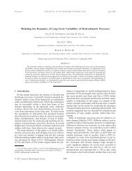
FIG. 1. Schematic <strong>of</strong> exact analytic solution <strong>of</strong> viscous <strong>Burgers</strong> equation at non-dimensional time t = 0.92,<br />
for Re = 10 and Re = 100. Discontinuous initial condition at t = 0 indicated by bold dashed line.<br />
where F(ξ; x, t) = ξ<br />
0 u0(ξ ′ ) dξ ′ + 0.5(x − ξ) 2 /t. The initial conditions on u(x, t) are<br />
given by u0(x) = u(x, 0) ={1if−1≤x≤0;or0if0
SYMBOLIC COMPUTATION OF THE BURGERS EQUATION 223<br />
nonlinearity <strong>of</strong> <strong>the</strong> equation and eliminates a large number <strong>of</strong> terms that would result o<strong>the</strong>rwise<br />
from <strong>the</strong> symbolic operations. Thus, (2) and (3) are modified to<br />
and<br />
∂u ′<br />
=−u′∂u′<br />
∂t ′<br />
∂x ′ +Re−1 ∂2 u ′<br />
, (2a)<br />
∂x ′2<br />
∂u ′<br />
=−u′∂u′<br />
∂t ′ ∂x ′.<br />
(3a)<br />
Integration <strong>of</strong> (2a) over a discrete time increment leads to <strong>the</strong> following exact, recursive<br />
expression, where <strong>the</strong> primes denoting non-dimensional variables have been dropped for<br />
convenience,<br />
uτ+1 = uτ <br />
+ t −u ∂u<br />
∂x + Re−1 ∂2u ∂x 2<br />
t<br />
. (6)<br />
The integration <strong>of</strong> (3a) differs only in <strong>the</strong> omission <strong>of</strong> <strong>the</strong> viscous term. In (6), t is <strong>the</strong> time<br />
increment, <strong>the</strong> superscript and overbar <strong>of</strong> <strong>the</strong> bracketed terms represent <strong>the</strong> time average<br />
over <strong>the</strong> time increment, and τ corresponds to <strong>the</strong> time step, in which τ = 0 initially. Thus,<br />
recursive application <strong>of</strong> (6) represents an exact analytic solution at discrete time steps, mt,<br />
where m is a positive integer.<br />
An iterative technique was developed to approximate (6), using a trapezoidal time averaging<br />
operator, in which equal weighting is given to <strong>the</strong> new and old time steps (i.e., effectively<br />
a Crank–Nicolson implicit approach applied to <strong>the</strong> symbolic integration). <strong>Symbolic</strong> computation<br />
<strong>of</strong> <strong>the</strong> spatial terms proceeds in a straightforward manner for each iteration in<br />
a given time step. To begin each time step in <strong>the</strong> recursion, <strong>the</strong> first iteration utilizes a<br />
forward-in-time operator as<br />
u τ+1<br />
∗<br />
= uτ <br />
+ t −u ∂u<br />
∂x + Re−1 ∂2u ∂x 2<br />
τ<br />
. (7a)<br />
That is, <strong>the</strong> time average <strong>of</strong> <strong>the</strong> bracketed derivative terms in (6) is initially approximated<br />
by <strong>the</strong> symbolic representation at time level τ. Then uτ+1 ∗ , <strong>the</strong> first iterative value <strong>of</strong> uτ+1 ,<br />
is obtained from (7a), and spatial derivatives are computed for time level τ + 1, based on<br />
uτ+1 ∗ . In <strong>the</strong> second iteration, <strong>the</strong> time average <strong>of</strong> <strong>the</strong> derivative terms is approximated by<br />
<strong>the</strong> arithmetic average <strong>of</strong> <strong>the</strong>ir symbolic representations at τ and τ + 1 to obtain an updated<br />
symbolic version <strong>of</strong> uτ+1 ,as<br />
u τ+1 =u τ + t<br />
−u<br />
2<br />
∂u<br />
∂x +Re−1 ∂2u ∂x 2<br />
τ <br />
∂u∗<br />
+ −u∗<br />
∂x + Re−1 ∂2u∗ ∂x 2<br />
τ+1 <br />
. (7b)<br />
Spatial derivatives at <strong>the</strong> τ + 1 time level <strong>the</strong>n can be updated, <strong>with</strong> values at <strong>the</strong> τ level<br />
being held constant, and <strong>the</strong> iterative process can be repeated <strong>with</strong> (7b). However, sensitivity<br />
tests <strong>with</strong> multiple iterations suggest that a single trapezoidal averaging application is<br />
sufficient. That is, only one forward-in-time and one trapezoidal computation are necessary<br />
at each time step. Additional iterations primarily produce higher order harmonics <strong>of</strong> negligible<br />
magnitude ra<strong>the</strong>r than improve solution accuracy. The overall procedure is applied
224 DERICKSON AND PIELKE, SR.<br />
recursively to obtain symbolic representations for each succeeding time level, i.e., u τ+2 ,<br />
u τ+3 , etc. The use <strong>of</strong> <strong>the</strong> iterative procedure yields a highly accurate, approximate analytic<br />
solution to <strong>the</strong> <strong>Burgers</strong> equation at <strong>the</strong> discrete time levels. Arbitrary accuracy is achieved<br />
by truncating only negligible high order terms during each time step.<br />
As will be discussed in greater detail in Subsection 3.3, <strong>the</strong> symbolic computations<br />
produce an increasing number <strong>of</strong> terms <strong>with</strong> each successive time step. After a few time<br />
steps <strong>the</strong> number <strong>of</strong> terms becomes massive (i.e., combinatorial explosion) and it is <strong>the</strong>refore<br />
routinely necessary to select and eliminate (i.e., filter) negligible terms <strong>of</strong> higher order<br />
during symbolic operations <strong>with</strong>in each time step. To ensure that eliminated terms are<br />
indeed negligible, it is necessary to establish upper numerical limits on A and t, and a<br />
lower limit on Re, points that will be addressed in Subsection 3.5.<br />
3.2. Overview <strong>of</strong> computational results. The symbolic solution <strong>of</strong> <strong>the</strong> <strong>Burgers</strong> equation<br />
was computed for seven discrete, non-dimensional time steps, which was sufficient to<br />
simulate <strong>the</strong> beginnings <strong>of</strong> <strong>the</strong> classic “sawtooth” waveform. It is important to emphasize<br />
that <strong>the</strong> seven non-dimensional time steps <strong>with</strong> <strong>the</strong> symbolic computations are equivalent to<br />
approximately 90 such time steps in a comparable numerical solution. This estimate is based<br />
on comparisons to numerical simulations <strong>of</strong> <strong>the</strong> <strong>Burgers</strong> equation performed by Derickson<br />
[10]. Whereas <strong>the</strong> magnitude <strong>of</strong> <strong>the</strong> time step, t, in numerical schemes is limited by severe<br />
restrictions on <strong>the</strong> upper bounds <strong>of</strong> <strong>the</strong> Fourier and Courant numbers, <strong>the</strong> symbolic solution,<br />
which is continuous in space, has no equivalent limitation. However, <strong>the</strong> ability to maintain<br />
solution accuracy while excluding negligible high order terms does restrict <strong>the</strong> numerical<br />
magnitude <strong>of</strong> t that can be applied to <strong>the</strong> symbolic solution.<br />
A very significant advantage <strong>of</strong> <strong>the</strong> symbolic approach over comparable numerical methods<br />
is that a numerical solution represents only a single parameter value (e.g., one value<br />
<strong>of</strong> Re), whereas <strong>the</strong> symbolic solution, being analytic, represents an infinite number <strong>of</strong><br />
parametric variations. Also, <strong>the</strong> lack <strong>of</strong> restriction on an upper limit <strong>of</strong> Re in <strong>the</strong> symbolic<br />
method adds a crucial advantage over numerical counterparts, such as DNS which is limited<br />
to Re ≤ 4000.<br />
All symbolic computations were performed <strong>with</strong> <strong>the</strong> MAPLE symbolic engine (Redfern<br />
[20]). Computations were done in a manual, interactive mode on a 90-MHZ PC, which<br />
possessed 32 megabits <strong>of</strong> RAM. To compute seven time steps took approximately 10 minutes,<br />
most <strong>of</strong> which were consumed by manual operations, computer I/O operations, and<br />
visual assessment <strong>of</strong> results at each intermediate symbolic operation. Actual computation<br />
time is estimated to be about 2 to 4 minutes. Future efforts <strong>with</strong> more computational power<br />
and memory, and <strong>with</strong> a fully automated computational process, will greatly extend <strong>the</strong><br />
preliminary results reported in this paper.<br />
Table I presents <strong>the</strong> symbolic results for <strong>the</strong> 1st and 3rd time steps, showing <strong>the</strong> birth and<br />
growth <strong>of</strong> harmonics and <strong>the</strong> decay <strong>of</strong> <strong>the</strong> fundamental <strong>with</strong> time. The table also reveals <strong>the</strong><br />
general form <strong>of</strong> <strong>the</strong> solution for each discrete time level, mt (m = 1, 2, 3,...,M),<br />
u(x, mt) =<br />
N<br />
Fn sin(nκx), (8)<br />
n=1<br />
where<br />
<br />
J<br />
Fn = Cn j An+2 j−2 κ n+2 j−3 t n+2 j−3 +<br />
j=1<br />
J<br />
j=1<br />
Dn j An+2 j−2 κ n+2 j−1 <br />
n+2 j−2 1<br />
t<br />
Re
SYMBOLIC COMPUTATION OF THE BURGERS EQUATION 225<br />
TABLE I<br />
Results <strong>of</strong> <strong>Symbolic</strong> Computation <strong>of</strong> <strong>the</strong> <strong>Burgers</strong> <strong>Equation</strong> for 1st and 3rd Time Steps<br />
[A] 1st Time Step<br />
Forward-in-time iteration<br />
<br />
A− Aκ2t 1<br />
<br />
sin(κx) −<br />
Re<br />
1<br />
2 A2κt sin(2κx)<br />
u(x,t)=<br />
Trapezoidal iteration<br />
<br />
u(x,t)= A− 1<br />
8 A3κ 2 t 2 <br />
+ −Aκ 2 t + 1<br />
8 A3κ 4 t 3<br />
<br />
1<br />
Re<br />
× sin(2κx) +<br />
<br />
3<br />
8 A3κ 2 t 2 − 3<br />
8 A3κ 4 3 1<br />
t<br />
Re<br />
<br />
sin(κx) + − 1<br />
2 A2κt + 3<br />
2 A2κ 3 <br />
2 1<br />
t<br />
Re<br />
<br />
sin(3κx) − 1<br />
8 A4 κ 3 t 3 sin(4κx)<br />
[B] 3rd Time Step<br />
Trapezoidal iteration<br />
<br />
u(x, 3t) = A − 9<br />
8 A3κ 2 t 2 − 3<br />
32 A5κ 4 t 4 <br />
+ −3Aκ 2 t + 75<br />
8 A3κ 4 t 3 + 383<br />
32 A5κ 6 t 5<br />
<br />
1<br />
sin(κx)<br />
Re<br />
<br />
+ − 3<br />
2 A2κt + 4A 4 κ 3 t 3 − 67<br />
128 A6κ 5 t 5 <br />
27<br />
+<br />
2 A2κ 3 t 2 −54A 4 κ 5 t 4 − 5175<br />
128 A6κ 7 t 6<br />
<br />
1<br />
Re<br />
<br />
27<br />
× sin(2κx)+<br />
8 A3κ 2 t 2 − 801<br />
64 A5κ 4 t 4 + 261<br />
64 A7κ 6 t 6 <br />
+ − 417<br />
8 A3κ 4 t 3 + 14349<br />
64 A5κ 6 t 5<br />
+ 11145<br />
128 A7κ 8 t 7<br />
<br />
1<br />
sin(3κx) + −<br />
Re<br />
67<br />
8 A4κ 3 t 3 + 1151<br />
32 A6κ 5 t 5 − 553<br />
32 A8κ 7 t 7<br />
<br />
363<br />
+<br />
2 A4κ 5 t 4 − 24567<br />
32 A6κ 7 t 6 − 3747<br />
64 A8κ 9 t 8<br />
<br />
1<br />
sin(4κx)<br />
Re<br />
⎧<br />
⎪⎨<br />
1365<br />
64<br />
+<br />
⎪⎩<br />
A5κ 4 t 4 − 6175<br />
64 A7κ 6 t 6 + 513265<br />
4096 A9κ 8 t 8<br />
<br />
+ − 36545<br />
64 A5κ 6 t 5 + 292585<br />
128 A7κ 8 t 7 − 11108435<br />
A<br />
4096<br />
9 κ 10 t 9<br />
⎫<br />
⎪⎬<br />
sin(5κx)<br />
1 ⎪⎭<br />
Re<br />
<br />
+ − 6855<br />
128 A6κ 5 t 5 + 22233<br />
128 A8κ 7 t 7 <br />
209829<br />
+<br />
128 A6κ 7 t 6 − 2263035<br />
A<br />
512<br />
8 κ 9 t 8<br />
<br />
1<br />
sin(6κx)<br />
Re<br />
is <strong>the</strong> amplitude <strong>of</strong> each harmonic at <strong>the</strong> discrete time level mt; n = 1, 2, 3,...,N corresponds<br />
to <strong>the</strong> fundamental and each harmonic up to <strong>the</strong> (N − 1)st harmonic; and <strong>the</strong> index<br />
j = 1, 2, 3,...,J corresponds to <strong>the</strong> respective terms associated <strong>with</strong> <strong>the</strong> fundamental and<br />
each harmonic. The fundamental is denoted by sin(κx) and <strong>the</strong> odd and even harmonics<br />
are denoted by sin{(2n)κx} and sin{(2n + 1)κx} , respectively. Thus, sin(2κx) corresponds<br />
to <strong>the</strong> 1st harmonic and sin(3κx) corresponds to <strong>the</strong> 2nd harmonic, etc. Cnj and Dnj, all<br />
<strong>of</strong> which are rational numbers, are <strong>the</strong> respective leading coefficients for each inviscid and<br />
viscous term. For convenience <strong>of</strong> analysis, <strong>the</strong> terms are viewed as inviscid-viscous pairs,<br />
(Cnj, Dnj), in which each pair <strong>of</strong> terms is denoted by its leading coefficients for expediency.<br />
Table I shows that at each time step <strong>the</strong> leading coefficients, Cnj and Dnj, <strong>of</strong> all existing<br />
terms change, and new terms are added to <strong>the</strong> fundamental and each harmonic through<br />
<strong>the</strong> symbolic computations. The table represents a filtered solution in which negligible<br />
higher order terms were excluded during computations. As can be observed in <strong>the</strong> table,<br />
leading coefficients can become quite large, complicating <strong>the</strong> issue <strong>of</strong> discerning negligible<br />
terms. The coefficients are rational numbers, which preserve solution accuracy. MAPLE<br />
can handle extremely large integers (500,000 digits), so large leading coefficients are not a<br />
computational problem.
226 DERICKSON AND PIELKE, SR.<br />
The symbolic solution represents an approximate, spatially continuous analytical solution<br />
<strong>of</strong> high order accuracy at discrete time levels. The forward-in-time iteration (FI) is included<br />
for <strong>the</strong> 1st time step in Table I to elucidate <strong>the</strong> process <strong>of</strong> solution improvement. Only<br />
<strong>the</strong> final, or trapezoidal, time iteration (TI) is shown for <strong>the</strong> 3rd time step. In general,<br />
higher order terms are affected most by <strong>the</strong> second iteration in <strong>the</strong> symbolic computations,<br />
a characteristic common to numerical iterations. Results for <strong>the</strong> inviscid <strong>Burgers</strong> equation<br />
differ from <strong>the</strong> tabulated viscous solution only in <strong>the</strong> exclusion <strong>of</strong> all terms containing Re.<br />
<strong>Symbolic</strong> computations are quicker and easier to perform for <strong>the</strong> inviscid case due to <strong>the</strong><br />
absence <strong>of</strong> <strong>the</strong> viscous terms, which cause considerably greater combinatorial interactions.<br />
However, <strong>the</strong> inviscid case, which corresponds to infinite Re, does not induce <strong>the</strong> instabilities<br />
inherent to numerical solutions at high Re.<br />
The symbolic solution does not produce false dispersion <strong>of</strong> waves or aliasing, nor require<br />
an upper bound on Re. These are significant issues in numerical methods. The analytic nature<br />
<strong>of</strong> <strong>the</strong> symbolic solution, which is continuous in space and discrete in time, precludes<br />
false dispersion and aliasing and any restriction on maximum allowable Re. These phenomena<br />
are known to be associated <strong>with</strong> spatial discretization in finite difference methods<br />
(e.g., Derickson [10]). Spectral methods, while producing minimal false dispersion, require<br />
dealiasing at each computational time step (e.g., Fletcher [14]). Spectral DHS methods also<br />
are restricted to Re values <strong>of</strong> no greater than 4000.<br />
As will be elaborated in Subsection 3.5, <strong>the</strong> viscous solution is valid only for Re above a<br />
lower limit <strong>of</strong> 500. For <strong>the</strong> solution to remain valid below this lower threshold, a large number<br />
<strong>of</strong> symbolic terms containing higher order powers <strong>of</strong> Re −1 must be retained in <strong>the</strong> symbolic<br />
computations, resulting in much greater computational expenditure. This happenstance is<br />
ironic in contrast to <strong>the</strong> difficulty numerical solutions face as Re increases from small to<br />
large magnitudes, <strong>the</strong> latter <strong>of</strong> which represent <strong>the</strong> more interesting regimes <strong>of</strong> turbulent<br />
flow, in general.<br />
Figures 2 and 3 show <strong>the</strong> evolution <strong>of</strong> <strong>the</strong> symbolic solution for Re = 500 and Re =∞<br />
(i.e., <strong>the</strong> inviscid case), respectively. The initial condition and <strong>the</strong> 3rd and 7th time steps<br />
are shown. Values <strong>of</strong> A = 0.3 and t = 0.055, which were determined to be appropriate<br />
upper numerical limits on <strong>the</strong> amplitude factor and non-dimensional time step to maintain<br />
solution validity, are reflected in <strong>the</strong> figures. The figures reveal <strong>the</strong> decay <strong>of</strong> <strong>the</strong> fundamental<br />
and <strong>the</strong> growth <strong>of</strong> harmonics, yielding a net waveform that is tending toward <strong>the</strong><br />
well known “sawtooth” shape produced in solutions to <strong>the</strong> <strong>Burgers</strong> equation at high Re.<br />
Figure 2, corresponding to Re = 500, shows greater damping <strong>of</strong> <strong>the</strong> fundamental and slower<br />
growth <strong>of</strong> <strong>the</strong> harmonics <strong>with</strong> time. However, <strong>the</strong> differences between <strong>the</strong> two cases become<br />
visibly discernible in Figs. 2 and 3 only at <strong>the</strong> 7th time step. As revealed in Table I and<br />
Figs. 2 and 3, <strong>the</strong> fundamental and <strong>the</strong> even harmonics have positive amplitudes and <strong>the</strong><br />
odd harmonics have negative amplitudes. This alternation <strong>of</strong> sign is more clearly shown in<br />
Fig. 4, which displays <strong>the</strong> growth <strong>of</strong> <strong>the</strong> harmonics <strong>with</strong> each successive time step. Figure<br />
4 also more clearly shows <strong>the</strong> greater harmonic magnitudes for Re =∞ compared to<br />
Re = 500.<br />
3.3. Combinatorics <strong>of</strong> nonlinear interactions. In <strong>the</strong> symbolic solution, <strong>the</strong> quadratic<br />
nonlinear interactions at each time step correspond to symbolic multiplication between<br />
momentum, represented by (8), and its derivative, i.e., u ∂u<br />
, in which multiplications between<br />
∂x<br />
all possible combinations <strong>of</strong> existing harmonic pairs are performed pair by pair. Referring<br />
to Appendix A and (8) for elucidation, a single nonlinear multiplication between any two
SYMBOLIC COMPUTATION OF THE BURGERS EQUATION 227<br />
FIG. 2. Time evolution <strong>of</strong> fundamental and 1st through 5th harmonics in symbolic computation <strong>of</strong> <strong>the</strong> <strong>Burgers</strong><br />
equation for Re = 500. Non-dimensional amplitude factor and time step are A = 0.3 and t = 0.055, respectively.<br />
harmonics can be represented by <strong>the</strong> general form<br />
Lc A n1+2 j1−2 n2+2 j2−2<br />
A sin(n1κ)cos(n2κ)<br />
= 1<br />
2 LcA n1+n2+2(j1+j2−2)<br />
[sin(n1 + n2)κ + sin(n1 − n2)κ], (9)<br />
where Lc is <strong>the</strong> leading coefficient, <strong>the</strong> ordered pair (n1, n2) denotes <strong>the</strong> respective<br />
wavenumbers <strong>of</strong> <strong>the</strong> two interacting harmonics, and j1 and j2 represent <strong>the</strong> particular<br />
term associated <strong>with</strong> each harmonic, that is, its leading term, or its 2nd or 3rd term, etc.<br />
(refer to Table I and (8) for clarity). As explained in Appendix A, <strong>the</strong> term sin(n1 + n2)κ
228 DERICKSON AND PIELKE, SR.<br />
FIG. 3. Time evolution <strong>of</strong> fundamental and 1st through 5th harmonics in symbolic computation <strong>of</strong> <strong>the</strong> <strong>Burgers</strong><br />
equation for infinite Re. Non-dimensional amplitude factor and time step are A = 0.3 and t = 0.055, respectively.<br />
in (9) represents outscatter, or “production” <strong>of</strong> a higher order harmonic, and sin(n1 − n2)κ<br />
represents backscatter to a lower order harmonic.<br />
In general, j1 = j2 more frequently than j1 = j2. If a multiplication involves <strong>the</strong> leading<br />
term for each harmonic in <strong>the</strong> pair, <strong>the</strong>n j1 = j2 = 1. The multiplication represented by (9)<br />
may involve two inviscid terms, two viscous terms, or one inviscid and one viscous term,<br />
such that any one <strong>of</strong> <strong>the</strong> following four combinations is possible for <strong>the</strong> resulting leading<br />
coefficient, Lc: Lc = Cn1 j 1 Cn2 j 2 , Lc = Dn1 j 1 Dn2 j 2 , Lc = Cn1 j 1 Dn2 j 2 , or Lc = Dn1 j 1 Cn2 j 2 . The<br />
wavenumber, κ, and <strong>the</strong> time increment, t, have been omitted as factors in (9) because,<br />
referring to (8), <strong>the</strong>ir respective powers depend on whe<strong>the</strong>r inviscid or viscous terms, or a
SYMBOLIC COMPUTATION OF THE BURGERS EQUATION 229<br />
FIG. 4. Amplitudes <strong>of</strong> 1st through 10th harmonics at each <strong>of</strong> seven discrete time steps in symbolic computation<br />
<strong>of</strong> <strong>the</strong> <strong>Burgers</strong> equation for (a) Re = 500 and (b) infinite Re. The artifice <strong>of</strong> continuous curve fitting between discrete<br />
harmonics helps to clarify harmonic growth in time.<br />
mix, are involved in <strong>the</strong> multiplication. Their inclusion is not essential for <strong>the</strong> discussion<br />
at hand. Three possibilities exist for a nonlinear interaction between two harmonics represented<br />
by <strong>the</strong> ordered pair, (n1, n2): (i) n1 > n2, in which case <strong>the</strong> outcome <strong>of</strong> backscatter<br />
has a positive sign, (ii) n1 < n2, backscatter is negative in sign, and (iii) n1 = n2, which represents<br />
a self- interaction <strong>of</strong> a harmonic (or <strong>the</strong> fundamental), producing outscatter but no<br />
backscatter. Outscatter is identical for cases (i) and (ii). Each nonlinear interaction between<br />
a given pair (n1, n2) produces both outscatter and backscatter, <strong>with</strong> <strong>the</strong> exception <strong>of</strong> case
230 DERICKSON AND PIELKE, SR.<br />
TABLE II<br />
Example <strong>of</strong> Terms Produced by Nonlinear Interaction and Their<br />
Simplification (11 Terms Produced in 2nd Iteration <strong>of</strong> 1st Time Step<br />
in <strong>Symbolic</strong> Computation)<br />
(1) A2k sin(kx)cos(kx) = 1<br />
2 A2k sin(2kx)<br />
{A}<br />
(2) −2A2k 3tRsin(kx)cos(kx) =−A2k3tRsin(2kx) {B} {C} ∗<br />
(3) −A3k 2t sin(kx)cos(2kx) =− 1<br />
2 A3k 2 tsin(3kx) + 1<br />
2 A3k 2 t sin(kx)<br />
{B} {C} ∗<br />
(4) − 1<br />
2 A3k 2 t sin(2kx)cos(kx) =− 1<br />
4 A3k 2 tsin(3kx) − 1<br />
4 A3k 2 t sin(kx)<br />
{D} {E} ∗<br />
(5)<br />
1<br />
2 A3k 4 t 2 R sin(2kx)cos(kx) = 1<br />
4 A3k 4 t 2 R sin(3kx) + 1<br />
4 A3k 4 t 2 R sin(kx)<br />
(6)<br />
1<br />
2 A4k 3 t 2 R sin(2kx)cos(2kx) = 1<br />
4 A4k 3 t 2 (7)<br />
R sin(4kx)<br />
A2k 5t 2 R2 sin(kx)cos(kx) = 1<br />
2 A2k 5 t 2 R 2 sin(2kx)<br />
{D} {E} ∗<br />
(8) A3k 4t 2 R sin(kx)cos(2kx) = 1<br />
2 A3k 4 t 2 R sin(3kx) − 1<br />
2 A3k 4 t 2 R sin(kx)<br />
(9) Ak2 R sin(kx) = same<br />
(10) −Ak4tR2sin(kx) = same<br />
(11) −2A2k 3tRsin(2kx) = same {A}<br />
∗ Denotes backscatter.<br />
Note. A, B, C, D, and E denote terms <strong>with</strong> common factors.<br />
(iii), and <strong>the</strong> resulting amplitudes are identical for outscatter and backscatter, as reflected<br />
in <strong>the</strong> amplitude factor on <strong>the</strong> RHS <strong>of</strong> (9),<br />
amplitude factor = A n1+n2+2( j1+ j2−2) . (10)<br />
A simple example elucidates <strong>the</strong> great number <strong>of</strong> multiplicative combinations that arise<br />
in <strong>the</strong> symbolic computations. If at <strong>the</strong> beginning <strong>of</strong> a given time step <strong>the</strong>re are 6 harmonics,<br />
plus <strong>the</strong> fundamental, and each has 4 terms, <strong>the</strong>n <strong>the</strong>re are a total <strong>of</strong> 4(6 + 1) = 28<br />
terms representing momentum. Therefore, <strong>the</strong> momentum multiplied by its derivative yields<br />
28 2 = 784 quadratic terms at <strong>the</strong> new time step. Additionally, 28 linear terms are generated<br />
from <strong>the</strong> second order term in <strong>the</strong> <strong>Burgers</strong> equation, for a total <strong>of</strong> 812 terms. Table II displays<br />
<strong>the</strong> 11 resulting terms produced by symbolic computation <strong>of</strong> <strong>the</strong> <strong>Burgers</strong> equation at <strong>the</strong><br />
second (i.e., final) iteration <strong>of</strong> <strong>the</strong> 1st time step. At this point, <strong>the</strong> total number <strong>of</strong> terms is<br />
quite small compared to subsequent time steps when combinatorial explosion occurs. Also<br />
shown in <strong>the</strong> table are <strong>the</strong> conversion <strong>of</strong> quadratic terms through use <strong>of</strong> a trigonometric<br />
identity, as described in Appendix A, and <strong>the</strong> combination <strong>of</strong> like terms. Outscatter and<br />
backscatter are denoted in <strong>the</strong> table. The first eight terms shown in <strong>the</strong> table result from<br />
nonlinear interactions and <strong>the</strong> last three terms stem solely from <strong>the</strong> linear viscous term <strong>of</strong> <strong>the</strong><br />
<strong>Burgers</strong> equation. An important aspect identified in <strong>the</strong> table is that <strong>the</strong> second term, which<br />
is a nonlinear inertial term, combines <strong>with</strong> <strong>the</strong> last term, a strictly linear term stemming<br />
from viscous damping. Thus, <strong>the</strong> interplay between inertial and viscous terms is revealed.
SYMBOLIC COMPUTATION OF THE BURGERS EQUATION 231<br />
The integer exponent <strong>of</strong> <strong>the</strong> amplitude factor, (10), embodies complex combinations <strong>of</strong><br />
harmonic interactions. Signifying <strong>the</strong> exponent as E = n1 + n2 + 2( j1 + j2 − 2) , several<br />
scenarios can be explored. If only <strong>the</strong> leading terms <strong>of</strong> an interacting harmonic pair are<br />
considered, <strong>the</strong>n j1 = j2 = 1, and <strong>the</strong> exponent reduces to E = n1 + n2. Various wavenumber<br />
pairs, (n1, n2), potentially comprise E. Obviously, <strong>the</strong> higher <strong>the</strong> value <strong>of</strong> E is, <strong>the</strong> greater<br />
<strong>the</strong> complexity. Except when n1 = n2, each ordered pair, (n1, n2), has a counterpart pair,<br />
(n2, n1), <strong>with</strong> <strong>the</strong> two elements in reversed order. This is evident in Table II, which shows<br />
that <strong>the</strong> companion pairs exist in separate terms that may or may not have common signs<br />
or multipliers. One pair <strong>of</strong> <strong>the</strong> set potentially yields an opposite sign in backscatter, which<br />
does not in general lead to canceling effects, as seen in <strong>the</strong> table. If n1 = n2, no backscatter<br />
is produced, as previously explained.<br />
If o<strong>the</strong>r than leading terms are considered in <strong>the</strong> preceding analysis (i.e., j1 = 1 and j2 = 1),<br />
<strong>the</strong>n <strong>the</strong> scenarios involving <strong>the</strong> exponent <strong>of</strong> <strong>the</strong> amplitude factor become more complex,<br />
but follow a similar line <strong>of</strong> reasoning. For example, assume j1 = 1 and j2 = 1 in (10).<br />
Since n1 + n2 = E − 2( j1 + j2 − 2), setting E = 14 and j1 + j2 = 5 yields n1 + n2 = 8.<br />
The companion harmonic pairs (i) (2, 6) and (6, 2), (ii) (3, 5) and (5, 3), and (iii) (4, 4)<br />
satisfy <strong>the</strong> criterion n1 + n2 = 8. But for each <strong>of</strong> <strong>the</strong>se, <strong>the</strong> following combinations <strong>of</strong> term<br />
pairs, [ j1, j2], satisfy j1 + j2 = 5: [1, 4], [4, 1], [2, 3], and [3, 2] in which element order in<br />
each pair is important. Because <strong>the</strong>re are a total <strong>of</strong> 5 harmonic pairs, and 4 term pairs for each<br />
harmonic pair, a total <strong>of</strong> 20 interactions satisfy <strong>the</strong> criterion E = 14. All <strong>of</strong> <strong>the</strong> harmonic<br />
pairs produce outscatter to <strong>the</strong> 7th harmonic, because n1 + n2 = 8, but <strong>the</strong> harmonic pairs<br />
(2, 6) and (6, 2) produce backscatter to <strong>the</strong> 3rd harmonic. The pairs (3, 5) and (5, 3) produce<br />
backscatter to <strong>the</strong> 1st harmonic, and (4, 4) produces no backscatter. It is evident <strong>the</strong>re is<br />
a large and complex combination <strong>of</strong> harmonic interactions at play in <strong>the</strong> solution to <strong>the</strong><br />
<strong>Burgers</strong> equation.<br />
Table III displays combinations <strong>of</strong> nonlinear harmonic interactions, (n1, n2), that potentially<br />
produce outscatter and backscatter in <strong>the</strong> fundamental and <strong>the</strong> 10 harmonics produced<br />
in <strong>the</strong> symbolic solution. However, <strong>the</strong> companion harmonic pairs denoted by (n2, n1) are<br />
omitted for presentational convenience, but self-interactions denoted by n1 = n2 are included.<br />
Note that outscatter combinations are fewer in number compared to backscatter<br />
combinations, and that <strong>the</strong> fundamental only experiences backscatter. However, solution<br />
TABLE III<br />
Combinations <strong>of</strong> Harmonic Pairs Producing Outscatter and Backscatter for Fundamental<br />
and Various Harmonics<br />
Affected Outscatter Backscatter<br />
harmonic combinations combinations<br />
Fundamental None (1,2) (2,3) (3,4) (4,5) (5,6) (6,7) (7,8) (8,9) (9,10) ...<br />
1st harmonic (1,1) (1,3) (2,4) (3,5) (4,6) (5,7) (6,8) (7,9) (8,10) (9,11) ...<br />
2nd harmonic (1,2) (1,4) (2,5) (3,6) (4,7) (5,8) (6,9) (7,10) (8,11) (9,12) ...<br />
3rd harmonic (1,3) (2,2) (1,5) (2,6) (3,7) (4,8) (5,9) (6,10) (7,11) (8,12) ...<br />
4th harmonic (1,4) (2,3) (1,6) (2,7) (3,8) (4,9) (5,10) (6,11) (7,12) (8,13) ...<br />
5th harmonic (1,5) (2,4) (3,3) (1,7) (2,8) (3,9) (4,10) (5,11) (6,12) (7,13) ...<br />
6th harmonic (1,6) (2,5) (3,4) (1,8) (2,9) (3,10) (4,11) (5,12) (6,13) (7,14) ...<br />
7th harmonic (1,7) (2,6) (3,5) (4,4) (1,9) (2,10) (3,11) (4,12) (5,13) (6,14) ...<br />
8th harmonic (1,8) (2,7) (3,6) (4,5) (1,10) (2,11) (3,12) (4,13) (5,14) (6,15) ...<br />
9th harmonic (1,9) (2,8) (3,7) (4,6) (5,5) (1,11) (2,12) (3,13) (4,14) (5,15) ...<br />
10th harmonic (1,10) (2,9) (3,8) (4,7) (5,6) (1,12) (2,13) (3,14) (4,15) (5,16) ...
232 DERICKSON AND PIELKE, SR.<br />
results presented in Subsection 3.4 show that most backscatter combinations are <strong>of</strong> negligible<br />
consequence. In contrast, all outscatter combinations are found to be significant, but<br />
<strong>the</strong> strongest effect always involves <strong>the</strong> fundamental.<br />
The preceding analysis provides a framework to analyze and interpret <strong>the</strong> results produced<br />
by <strong>the</strong> symbolic computation <strong>of</strong> <strong>the</strong> <strong>Burgers</strong> equation. Referring to (8), each <strong>of</strong> <strong>the</strong><br />
J inviscid and J viscous terms comprising <strong>the</strong> amplitude, Fn, <strong>of</strong> each harmonic in <strong>the</strong><br />
symbolic solution is itself a composite which embodies outscatter, backscatter, and viscous<br />
damping that result from potentially large numbers <strong>of</strong> interacting harmonic pairs. It<br />
is instructive to examine individual effects that lead to each composite term in Fn by investigating<br />
intermediate symbolic operations during each time step, similarly to what was<br />
described for Table II. Such a task is useful, in general, for identifying and studying various<br />
nonlinear inertial interactions, linear damping mechanisms, and <strong>the</strong> interplay between<br />
inertia and viscous damping. However, experience indicates that it would be inefficient,<br />
if not intractable, to use <strong>the</strong> intermediate symbolic operations if <strong>the</strong> goal is to isolate and<br />
assess <strong>the</strong> integrated individual effects <strong>of</strong> outscatter, backscatter, and viscous damping on<br />
each individual harmonic. Therefore, an efficient, supplemental method is developed in<br />
Appendix B to achieve <strong>the</strong> desired result <strong>of</strong> isolating and separately evaluating <strong>the</strong> effects<br />
<strong>of</strong> <strong>the</strong>se three key mechanisms.<br />
3.4. Detailed symbolic results: Analysis <strong>of</strong> outscatter, backscatter, and viscous damping.<br />
In viewing <strong>the</strong> symbolic results embodied in Tables I and II, it is useful to explore <strong>the</strong> fundamental<br />
and various harmonics separately. At each time step, <strong>the</strong> symbolic solution, which is<br />
in <strong>the</strong> form expressed by (8), is post-processed using <strong>the</strong> method presented in Appendix B<br />
in which <strong>the</strong> following numerical upper limits are applied: A = 0.3, and t = 0.55. The<br />
process <strong>of</strong> determining appropriate numerical values is described in Subsection 3.5.<br />
Figures 5–8 show <strong>the</strong> evolution <strong>of</strong> <strong>the</strong> fundamental and <strong>the</strong> 1st, 3rd, and 10th harmonics<br />
over <strong>the</strong> seven computed time steps. The fundamental and specific harmonics were chosen<br />
to enable a broad analysis and interpretation <strong>of</strong> <strong>the</strong> fundamental results <strong>of</strong> <strong>the</strong> symbolic<br />
solution. The symbols Oni −n j and Bni −n are employed in <strong>the</strong> figures to represent <strong>the</strong><br />
j<br />
outscatter (i.e., production) and backscatter, and <strong>the</strong> specific harmonic pairs leading to<br />
each effect. Onet and Bnet denote <strong>the</strong> net effects <strong>of</strong> outscatter and backscatter. The viscous<br />
damping <strong>of</strong> <strong>the</strong> fundamental and three harmonics is shown separately on <strong>the</strong> figures and<br />
labeled explicitly. Each figure shows results for (a) Re = 500 and (b) Re =∞. Care must be<br />
exercised in comparing Figs. 5–8, because <strong>the</strong> vertical scales differ between each figure to<br />
accommodate <strong>the</strong> range <strong>of</strong> magnitudes <strong>of</strong> <strong>the</strong> outscatter, backscatter, and damping for each<br />
respective harmonic being displayed. For direct comparison between harmonics, <strong>the</strong> reader<br />
is referred to Figs. 4 and 9 in which all harmonics are displayed on <strong>the</strong> same vertical scale.<br />
Figure 5 displays solution results for <strong>the</strong> fundamental. The greatest backscatter, denoted<br />
by B1−2, stems from <strong>the</strong> nonlinear interaction between <strong>the</strong> 1st harmonic and <strong>the</strong> fundamental<br />
itself. Secondary backscatter occurs through interactions between <strong>the</strong> 1st and 2nd<br />
harmonics, B2−3, and between <strong>the</strong> 2nd and 3rd harmonics, B3−4. Backscatter also results<br />
from interactions between <strong>the</strong> 3rd and 4th harmonics and o<strong>the</strong>r higher order pairs differing<br />
by κ in wavenumber, but those interactions are negligible and not shown on <strong>the</strong> figure. When<br />
Re = 500, viscous damping exceeds <strong>the</strong> primary backscatter in magnitude up until <strong>the</strong> 2nd<br />
time step, beyond which <strong>the</strong> backscatter increases significantly in magnitude due to <strong>the</strong> rapid<br />
growth <strong>of</strong> <strong>the</strong> 1st harmonic. The effect <strong>of</strong> damping slowly decreases <strong>with</strong> each time step as<br />
<strong>the</strong> amplitude <strong>of</strong> <strong>the</strong> fundamental decreases, but always exceeds <strong>the</strong> secondary backscatter.
SYMBOLIC COMPUTATION OF THE BURGERS EQUATION 233<br />
FIG. 5. The time evolution <strong>of</strong> <strong>the</strong> fundamental at each <strong>of</strong> seven discrete time steps in symbolic computation <strong>of</strong><br />
<strong>the</strong> <strong>Burgers</strong> equation for (a) Re = 500 and (b) infinite Re. Displays backscatter, Bn1-n2, resulting from interactions<br />
between specific harmonic pairs, (n1,n2), and damping due to viscosity. Example B2-3 represents backscatter due<br />
to interaction between 1st and 2nd harmonics.<br />
In all cases, both damping and backscatter diminish <strong>the</strong> magnitude <strong>of</strong> <strong>the</strong> fundamental.<br />
There is no outscatter to <strong>the</strong> fundamental due to <strong>the</strong> absence <strong>of</strong> lower order harmonics.<br />
When Re =∞, <strong>the</strong>re is no damping, but by comparing parts (a) and (b) <strong>of</strong> Fig. 5, it is<br />
apparent that <strong>the</strong> effects <strong>of</strong> backscatter increase by only a small amount. Thus, viscosity<br />
does not have a large influence on <strong>the</strong> fundamental over <strong>the</strong> seven time steps computed.<br />
The 1st harmonic reveals more intricate behavior. Time histories <strong>of</strong> <strong>the</strong> production (i.e.,<br />
outscatter), backscatter, and viscous damping are displayed in Fig. 6. The 1st harmonic is<br />
created at <strong>the</strong> 1st time step by self-interaction <strong>of</strong> <strong>the</strong> fundamental, as denoted by O1−1 in<br />
<strong>the</strong> figure, and continues to grow <strong>with</strong> time, but at a decreasing rate as <strong>the</strong> fundamental<br />
diminishes. Being an odd harmonic, its amplitude is negative. Its only mode <strong>of</strong> production<br />
is through <strong>the</strong> fundamental, but it experiences backscatter due to interaction between <strong>the</strong><br />
fundamental and 2nd harmonic, noted by B1−3 in <strong>the</strong> figure, and between <strong>the</strong> 1st and<br />
3rd harmonics, shown as B2−4. O<strong>the</strong>r modes <strong>of</strong> backscatter are negligible and not shown.<br />
Production swamps backscatter and damping over all seven time steps. Backscatter and
234 DERICKSON AND PIELKE, SR.<br />
FIG. 6. The time evolution <strong>of</strong> <strong>the</strong> 1st harmonic. Displays backscatter, Bn1-n2, and outscatter, Om1-m2, resulting<br />
from interactions between specific harmonic pairs, (n1,n2) and (m1,m2), and damping due to viscosity. Example<br />
B1-3 represents backscatter due to interaction between fundamental and 2nd harmonic.<br />
damping serve to diminish <strong>the</strong> amplitude <strong>of</strong> <strong>the</strong> 1st harmonic, and damping increases <strong>with</strong><br />
time because <strong>the</strong> harmonic is growing.<br />
When Re =∞, <strong>the</strong>re is no damping, but production and backscatter increase by only a<br />
small amount, as shown in Fig. 8. Like <strong>the</strong> fundamental, <strong>the</strong> 1st harmonic is affected more<br />
by inviscid mechanisms than by viscosity throughout <strong>the</strong> time evolution <strong>of</strong> <strong>the</strong> symbolic<br />
computation.<br />
Bypassing <strong>the</strong> 2nd harmonic, an analysis is made <strong>of</strong> <strong>the</strong> 3rd harmonic due to its greater<br />
complexity. While <strong>the</strong> 2nd harmonic is created solely by interactions between <strong>the</strong> fundamental<br />
and <strong>the</strong> 1st harmonic, <strong>the</strong> 3rd harmonic is created from outscatter produced by two<br />
distinct pairs <strong>of</strong> interactions: (a) <strong>the</strong> fundamental and <strong>the</strong> 2nd harmonic, and (b) <strong>the</strong> selfinteractions<br />
<strong>of</strong> <strong>the</strong> 1st harmonic. The two production mechanisms are represented by O1−3<br />
and O2−2 in Fig. 7, in which O1−3 is nearly three times as large as O2−2 for all seven time<br />
steps. It may seem counterintuitive that O1−3 should be that much greater than O2−2,given<br />
that <strong>the</strong> 1st harmonic is straddled by an interaction that produces a greater effect than its<br />
own self-interaction. The explanation lies in <strong>the</strong> large amplitude, F1, <strong>of</strong> <strong>the</strong> fundamental,<br />
such that |F1F3| > 1<br />
2 F 2 2 , (see discussion in Appendix B).
SYMBOLIC COMPUTATION OF THE BURGERS EQUATION 235<br />
FIG. 7. The time evolution <strong>of</strong> <strong>the</strong> 3rd harmonic. Displays outscatter, backscatter, and viscous damping.<br />
Backscatter to <strong>the</strong> 3rd harmonic occurs due to interaction between <strong>the</strong> fundamental and<br />
4th harmonic and between <strong>the</strong> 1st and 5th harmonics, as shown in Fig. 7 by B1−5 and B2−6,in<br />
which B1−5 ≫ B2−6. All higher order backscatter is negligible and <strong>the</strong>refore excluded. The<br />
net effect <strong>of</strong> backscatter is about one-fourth that <strong>of</strong> production, but damping is comparable<br />
in magnitude to primary backscatter, so <strong>the</strong> net effect <strong>of</strong> backscatter and damping is quite<br />
significant on <strong>the</strong> 3rd harmonic.<br />
Lack <strong>of</strong> damping at Re =∞has a more significant effect on <strong>the</strong> 3rd harmonic than for<br />
<strong>the</strong> lower order harmonics and <strong>the</strong> fundamental, as shown in Fig. 7. Beginning <strong>with</strong> <strong>the</strong><br />
3rd harmonic, <strong>the</strong> solution revealed that <strong>the</strong> lack <strong>of</strong> viscosity has an increasingly pr<strong>of</strong>ound<br />
effect on both production and backscatter <strong>with</strong> increasing harmonic order, <strong>with</strong> <strong>the</strong> strongest<br />
impact being on backscatter. Results for higher order harmonics are not displayed.<br />
Analysis also reveals that for each successively higher order harmonic, <strong>the</strong> role <strong>of</strong> damping<br />
increases to <strong>the</strong> point <strong>of</strong> exceeding <strong>the</strong> effect <strong>of</strong> backscatter, and <strong>the</strong> combination <strong>of</strong> damping<br />
and backscatter becomes increasingly significant relative to <strong>the</strong> net effect <strong>of</strong> production.<br />
This is certainly an intuitive result. The ratio <strong>of</strong> <strong>the</strong> magnitude <strong>of</strong> production to <strong>the</strong> combined<br />
magnitude <strong>of</strong> damping and backscatter, however, is about three for <strong>the</strong> 8th harmonic. Thus,<br />
production, or outscatter, continues to play <strong>the</strong> dominant role.
236 DERICKSON AND PIELKE, SR.<br />
FIG. 8. The time evolution <strong>of</strong> <strong>the</strong> 10th harmonic. Displays outscatter and viscous damping. Being <strong>the</strong> highest<br />
order harmonic in <strong>the</strong> symbolic solution, no backscatter is present.<br />
More modes <strong>of</strong> production are present <strong>with</strong> increasing harmonic order, as evident in <strong>the</strong><br />
figures and in Table III, due to <strong>the</strong> greater number <strong>of</strong> associated lower order harmonics.<br />
Thus, while <strong>the</strong> 5th harmonic has three production modes, <strong>the</strong> 7th harmonic has four. By <strong>the</strong><br />
9th and 10th harmonics <strong>the</strong>re are five modes <strong>of</strong> production, as shown in Fig. 8 for <strong>the</strong> 10th<br />
harmonic. The strongest, or primary, mode <strong>of</strong> production was found to always involve <strong>the</strong><br />
fundamental. Each individual secondary mode <strong>of</strong> production is smaller in magnitude than <strong>the</strong><br />
primary mode. With increasing harmonic order, however, <strong>the</strong>re are more secondary modes<br />
and collectively <strong>the</strong>y can produce a greater effect than <strong>the</strong> primary mode <strong>of</strong> production.<br />
It is <strong>the</strong>refore apparent that as time evolves and additional higher order harmonics are<br />
produced, <strong>the</strong> mechanisms <strong>of</strong> outscatter become increasingly numerous and complex. On<br />
<strong>the</strong> o<strong>the</strong>r hand, <strong>the</strong>re are at most only two significant backscatter combinations for all <strong>the</strong><br />
harmonics produced in <strong>the</strong> symbolic solution, and only one <strong>of</strong> those has a primary effect.<br />
The 9th harmonic has only one backscatter mode and <strong>the</strong> 10th harmonic has none, as will<br />
be discussed subsequently.<br />
Three key facts emerge regarding <strong>the</strong> mechanisms and behavior <strong>of</strong> backscatter in <strong>the</strong><br />
symbolic solution <strong>of</strong> <strong>the</strong> <strong>Burgers</strong> equation. First <strong>of</strong> all, significant backscatter to each harmonic<br />
except <strong>the</strong> 1st results solely from interactions between a harmonic pair containing a<br />
lower order harmonic and a higher order harmonic relative to <strong>the</strong> harmonic being influenced.
SYMBOLIC COMPUTATION OF THE BURGERS EQUATION 237<br />
FIG. 9. The comparative amplitudes <strong>of</strong> <strong>the</strong> fundamental and 1st through 10th harmonics at each <strong>of</strong> seven<br />
discrete time steps in symbolic computation <strong>of</strong> <strong>the</strong> <strong>Burgers</strong> equation for (a) Re = 500 and (b) infinite Re. The slope<br />
<strong>of</strong> each curve reveals <strong>the</strong> time rate <strong>of</strong> change <strong>of</strong> each harmonic.<br />
In all cases observed, <strong>the</strong> fundamental interacting <strong>with</strong> <strong>the</strong> adjacent higher order harmonic<br />
creates <strong>the</strong> dominant backscatter effect. Thus backscatter cannot be characterized as a “localized”<br />
nonlinear effect. Backscatter due to interactions in which both harmonics in <strong>the</strong><br />
pair are <strong>of</strong> higher order than <strong>the</strong> affected harmonic was found to be negligible in <strong>the</strong> preliminary<br />
computations. This certainly may not be <strong>the</strong> case for solutions <strong>with</strong> initial conditions<br />
that contain high order harmonics <strong>of</strong> large amplitude. There may be o<strong>the</strong>r cases where <strong>the</strong><br />
cumulative backscatter created by a myriad <strong>of</strong> high order pairs could be significant. Second,<br />
<strong>the</strong> effect <strong>of</strong> backscatter is to deplete momentum in all cases, regardless <strong>of</strong> <strong>the</strong> value <strong>of</strong> Re.
238 DERICKSON AND PIELKE, SR.<br />
Thus, viscous damping and backscatter work in concert to decrease <strong>the</strong> momentum. For<br />
time evolution beyond <strong>the</strong> current preliminary results, <strong>the</strong>re may be cases where <strong>the</strong> effect<br />
<strong>of</strong> backscatter is to supply momentum to lower order harmonics and <strong>the</strong> fundamental. Third,<br />
as <strong>the</strong> symbolic solution evolves, <strong>the</strong> highest order harmonic included at any given time step<br />
experiences production but no backscatter because <strong>of</strong> <strong>the</strong> absence <strong>of</strong> <strong>the</strong> next higher order<br />
harmonic. This is illustrated in Fig. 8 for <strong>the</strong> 10th harmonic, <strong>the</strong> highest order considered<br />
in <strong>the</strong> solution.<br />
It is argued that <strong>the</strong> unavoidable exclusion <strong>of</strong> backscatter for <strong>the</strong> highest order harmonic<br />
is <strong>of</strong> negligible consequence to <strong>the</strong> symbolic solution. First <strong>of</strong> all, by virtue <strong>of</strong> <strong>the</strong> filtering<br />
process described in Subsection 3.5, <strong>the</strong> amplitude <strong>of</strong> <strong>the</strong> highest order harmonic included in<br />
<strong>the</strong> solution at each time step is inherently small. Each successive higher order harmonic is<br />
allowed into <strong>the</strong> solution only when production (i.e., outscatter) causes <strong>the</strong> current highest<br />
order harmonic to exceed a certain magnitude relative to its lower order neighbor. The<br />
two primary ways <strong>the</strong> highest order harmonic affects <strong>the</strong> solution is through backscatter<br />
to its lower order neighbor and production to <strong>the</strong> next higher order harmonic. As was<br />
described in <strong>the</strong> preceding discussion, backscatter depletes momentum, at least for <strong>the</strong><br />
preliminary computations undertaken in this study. Thus, <strong>the</strong> lack <strong>of</strong> backscatter to <strong>the</strong><br />
highest order harmonic serves to make its amplitude somewhat larger than it o<strong>the</strong>rwise<br />
would be. Through backscatter, it <strong>the</strong>refore causes its lower order neighbor to be somewhat<br />
smaller than o<strong>the</strong>rwise. Then, because production <strong>of</strong> <strong>the</strong> highest order harmonic is directly<br />
related to <strong>the</strong> magnitude <strong>of</strong> its lower order neighbor, it in turn receives less production and<br />
grows less in amplitude. So <strong>the</strong> tendency <strong>of</strong> <strong>the</strong> highest order harmonic to become too large<br />
due to its not receiving backscatter is counteracted by a self-adjusting process. A more<br />
rigorous validation <strong>of</strong> solution accuracy, <strong>with</strong> truncation <strong>of</strong> higher order harmonics, is that<br />
<strong>the</strong> kinetic energy <strong>of</strong> <strong>the</strong> symbolic solution <strong>of</strong> <strong>the</strong> inviscid <strong>Burgers</strong> equation (i.e., Re =∞)<br />
was found to remain constant to <strong>with</strong>in 0.14% as <strong>the</strong> solution progressed in time. Thus<br />
energy is conserved to a high order <strong>of</strong> accuracy.<br />
Figure 9 displays <strong>the</strong> “birth” and growth <strong>of</strong> <strong>the</strong> 10 harmonics produced by <strong>the</strong> solution.<br />
The fundamental is excluded from <strong>the</strong> figure. The 4th harmonic is “born” at <strong>the</strong> 3rd time<br />
step and its growth accelerates in time. The 7th harmonic is born at <strong>the</strong> 4th time step when<br />
Re =∞, and at <strong>the</strong> 5th time step when Re = 500. The figure clearly reveals <strong>the</strong> enhanced<br />
effect <strong>of</strong> viscous damping <strong>with</strong> increasing harmonic order.<br />
3.5. Filtering negligible symbolic terms. As previously discussed, <strong>the</strong> symbolic results<br />
displayed in Tables I and II represent a filtered set <strong>of</strong> computations. Sensitivity tests were<br />
done in an attempt to develop an effective process to identify and eliminate negligible terms<br />
prior to symbolic multiplication in order to prevent or minimize unproductive combinatorial<br />
explosion and maintain solution accuracy. However, a significant portion <strong>of</strong> <strong>the</strong> filtering<br />
process can only be performed after symbolic operations have produced a myriad <strong>of</strong> both<br />
critical and superfluous terms. Filtering is based primarily on evaluating <strong>the</strong> symbolic terms<br />
comprising <strong>the</strong> amplitudes <strong>of</strong> <strong>the</strong> fundamental and each harmonic. The separate issue <strong>of</strong> <strong>the</strong><br />
addition, or “birth,” <strong>of</strong> higher order harmonics into <strong>the</strong> symbolic solution was described in<br />
Subsection 3.4.<br />
In (8) it is apparent that <strong>the</strong> leading inviscid and viscous terms for each harmonic are<br />
n 1<br />
Re<br />
Cn1 Anκ n−1t n−1 and Dn1 Anκ n+1t , in which Cn1 and Dn1 are <strong>the</strong>ir leading coefficients.<br />
The second inviscid and viscous terms are Cn2 An+2κ n+1t n+1 and Dn2 An+2κ n+3 n+2 1<br />
t Re ,<br />
<strong>with</strong> leading coefficients Cn2 and Dn2 . The relationship is identical for all successive terms
SYMBOLIC COMPUTATION OF THE BURGERS EQUATION 239<br />
considered. In evaluating <strong>the</strong> magnitude <strong>of</strong> terms at each time step, all terms are compared<br />
by ratio to <strong>the</strong>ir respective lead term (i.e., inviscid and viscous terms are treated separately).<br />
The exception is <strong>the</strong> fundamental for which <strong>the</strong> lead term is A, <strong>the</strong> initial amplitude. Thus<br />
all terms for <strong>the</strong> fundamental are compared instead to <strong>the</strong> 2nd inviscid term, C12 A3 κ 2 t 2 .<br />
For all harmonics, <strong>the</strong> resulting ratios, RatioI and RatioV , are as follows for <strong>the</strong> inviscid<br />
and viscous terms, respectively,<br />
and<br />
RatioI = Cn j<br />
Cn1<br />
RatioV = Dn j<br />
Dn1<br />
[Aκt] 2j−2<br />
[Aκt] 2j−2<br />
(11a)<br />
(11b)<br />
<strong>with</strong> j = 2, 3, 4,...,J. As will be discussed, Aκt ≪1. This composite factor, which<br />
appears in brackets in (11a) and (11b), is raised to an additional power <strong>of</strong> two for each<br />
successive higher order term being compared to <strong>the</strong> leading term. The magnitudes <strong>of</strong> <strong>the</strong><br />
coefficient ratios Cn j /Cn1 and Dn /Dn1 in (11a) and (11b) play a definitive role in discerning<br />
j<br />
whe<strong>the</strong>r a higher order term is negligible and can be excluded from <strong>the</strong> symbolic solution<br />
at any given time step.<br />
The filtering process implicitly requires upper numerical limits on A and t, and a lower<br />
limit on Re in order to evaluate <strong>the</strong> relative magnitudes <strong>of</strong> higher order symbolic terms<br />
and to establish <strong>the</strong> range <strong>of</strong> numerical parameters for which <strong>the</strong> symbolic solution applies.<br />
Higher order terms were eliminated if it was determined that <strong>the</strong>ir absence would not<br />
compromise <strong>the</strong> cumulative accuracy <strong>of</strong> subsequent symbolic operations. Sensitivity tests<br />
indicate that setting RatioI = RatioV ≈ 0.01 yields an effective filtering criterion. Given<br />
this criterion, appropriate upper numerical limits were determined for <strong>the</strong> initial amplitude,<br />
A, and <strong>the</strong> non-dimensional time step, t, asA≤0.3and t ≤ 0.055. Because <strong>the</strong> nondimensional<br />
wavenumber is large, i.e., κ = 2π, <strong>the</strong> preceding limits on t and A assure that<br />
Aκt ≪1, which reduces <strong>the</strong> magnitude <strong>of</strong> higher order terms and enables <strong>the</strong>ir truncation<br />
<strong>with</strong>out compromising <strong>the</strong> validity <strong>of</strong> <strong>the</strong> symbolic solution. In fact, Aκt ≈0.1, such that<br />
any combination <strong>of</strong> A and t that satisfies At ≈ 0.1/2π provides similar results when<br />
substituted into <strong>the</strong> symbolic solution. That is, a larger (smaller) A accompanies a smaller<br />
(larger) t, but <strong>the</strong> character <strong>of</strong> <strong>the</strong> generated waveform and <strong>the</strong> relationship between <strong>the</strong><br />
fundamental and harmonics remain similar. If one were to seek some combination <strong>of</strong> A and<br />
t which yielded Aκt >0.1, it would be necessary to retain a greater number <strong>of</strong> higher<br />
order terms as compensation. The goal is to maximize accuracy <strong>with</strong> <strong>the</strong> symbolic solution<br />
<strong>with</strong> a minimum number <strong>of</strong> terms.<br />
Numerical values <strong>of</strong> A, t, and Re are not used, <strong>of</strong> course, in <strong>the</strong> symbolic computations.<br />
However, once <strong>the</strong> symbolic solution is obtained, appropriate numerical values can be<br />
substituted for t, A, Re, and x, <strong>with</strong>in <strong>the</strong>ir appropriate ranges, to explore numerical<br />
implications <strong>of</strong> <strong>the</strong> solution. Note that <strong>the</strong> spatial variable, x, is also non-dimensional and<br />
falls in <strong>the</strong> range 0 ≤ x ≤ 1. As mentioned in Subsection 3.2, <strong>the</strong> symbolic solution <strong>of</strong><br />
<strong>the</strong> <strong>Burgers</strong> equation presents no upper limit to Re, but requires that Re ≥ 500. Extending<br />
<strong>the</strong> symbolic solution to lower values <strong>of</strong> Re would require retention <strong>of</strong> viscous terms <strong>of</strong><br />
O(1/Re) 2 or higher. <strong>Symbolic</strong> computation reveals that terms <strong>of</strong> O(1/Re) 2 have <strong>the</strong> form<br />
En j An+2 j−2κ n+2 j+1t n+2 j−1 (1/Re) 2 , yielding a ratio <strong>of</strong> (En j /Dn j )κ2t(1/Re) to terms<br />
<strong>of</strong> O(1/Re) in (8). To justify <strong>the</strong> exclusion <strong>of</strong> <strong>the</strong> higher order terms, <strong>the</strong> ratio must be small.
240 DERICKSON AND PIELKE, SR.<br />
A reasonable criterion is that (En j /Dn j )κ2t(1/Re) ≈ 0.1 as an upper limit. Thus, if En j<br />
and Dn were <strong>of</strong> equal magnitude, <strong>the</strong> lower limit on Reynolds number would be Re ≥ 20.<br />
j<br />
However, <strong>the</strong> symbolic results indicate that a more typical representative ratio between <strong>the</strong><br />
leading coefficients is En j /Dn ≈ 40, in which case <strong>the</strong> lower limit on Reynolds number<br />
j<br />
would be Re ≥ 900. Sensitivity runs <strong>with</strong> <strong>the</strong> symbolic computations, however, showed an<br />
effective limit to be Re ≥ 500. Highest order harmonics are most sensitive to <strong>the</strong> exclusion<br />
<strong>of</strong> O(1/Re) 2 terms. For longer time evolution <strong>the</strong>se terms, and possibly even higher order<br />
ones, must be retained. Therefore, it is clear that efforts exploring low Re flows would<br />
require solution refinements. Also, current results suggest that longer time evolution <strong>with</strong><br />
high values <strong>of</strong> Re may confront <strong>the</strong> need to retain O(1/Re) 2 terms to maintain solution<br />
accuracy, as well. The inclusion <strong>of</strong> more terms increases <strong>the</strong> computational complexity and<br />
intensifies combinatorial explosion. Thus, we face <strong>the</strong> irony that while numerical solutions<br />
experience instabilities <strong>with</strong> high Re flows, <strong>the</strong> symbolic approach has difficulty <strong>with</strong> low<br />
Re but can inherently handle flows <strong>with</strong> infinite Re. This is fortuitous because turbulent<br />
flows at extremely high values <strong>of</strong> Re are <strong>the</strong> most elusive and interesting in research and in<br />
practical applications.<br />
4. SUMMARY AND CONCLUSIONS<br />
A novel approach based on recursive symbolic computation is introduced for <strong>the</strong> approximate<br />
analytic solution <strong>of</strong> both <strong>the</strong> inviscid and viscous <strong>Burgers</strong> equations. Through<br />
<strong>the</strong> recursive process, symbolic representations <strong>of</strong> momentum are obtained continuously in<br />
space at discrete increments in time. Although approximate, <strong>the</strong> solution can be obtained to<br />
arbitrary, high order accuracy. Once obtained, appropriate numerical values can be inserted<br />
into <strong>the</strong> symbolic solution to explore parametric variations.<br />
The symbolic computations allow examination <strong>of</strong> <strong>the</strong> solution at stages prior to combining<br />
and simplifying terms during each time step. Thus, one can gain a deeper understanding<br />
<strong>of</strong> <strong>the</strong> precise role and character <strong>of</strong> all nonlinear interactions, viscous damping, and <strong>the</strong><br />
interplay between inertial and viscous mechanisms. This is not done easily, if at all, <strong>with</strong><br />
numerical solutions, which produce only <strong>the</strong> net effect <strong>of</strong> nonlinear interactions and o<strong>the</strong>r<br />
physical processes. Likewise, <strong>the</strong> ability to readily isolate and assess <strong>the</strong> integrated individual<br />
effects <strong>of</strong> outscatter, backscatter, and viscous damping by post-processing symbolic<br />
results lends power over numerical methods. The same basic arguments apply in comparing<br />
symbolic computation <strong>with</strong> traditional nonlinear analytical solutions. An added feature <strong>of</strong><br />
<strong>the</strong> symbolic approach is that “turbulence” manifests as a process <strong>of</strong> combinatorics, providing<br />
a fresh view to a classical problem, even though results are limited to <strong>the</strong> 1-D <strong>Burgers</strong><br />
equation. Based on <strong>the</strong> preliminary efforts presented, it appears that symbolic computation<br />
may be quite effective in unveiling <strong>the</strong> “anatomy” <strong>of</strong> <strong>the</strong> myriad inertial and viscous<br />
interactions that underlie fundamental turbulent behavior.<br />
Because <strong>of</strong> <strong>the</strong> tendency <strong>of</strong> nonlinear symbolic operations to produce combinatorial<br />
explosion, future efforts will require <strong>the</strong> development <strong>of</strong> improved filtering processes to<br />
select and eliminate negligible high order terms. Thus, while <strong>the</strong> preliminary results are<br />
limited to relatively short time evolution, it is envisioned that future efforts will explore<br />
more fully developed flows. With fur<strong>the</strong>r research, <strong>the</strong>re may be potential to extend <strong>the</strong><br />
symbolic computations to 2-D and 3-D studies.<br />
The symbolic approach is superior to numerical techniques in four distinct ways: (a) its<br />
ability to reveal and elucidate direct nonlinear interactions between waveforms, including
SYMBOLIC COMPUTATION OF THE BURGERS EQUATION 241<br />
<strong>the</strong> interplay between inertia and viscosity; (b) its ability to broadly explore parameter space,<br />
most importantly variations in Re, by simple substitution <strong>of</strong> desired numerical values into<br />
<strong>the</strong> analytical solution; (c) its ability to deal <strong>with</strong> a wide range <strong>of</strong> Re flows (500 ≤ Re ≤∞);<br />
and (d) it produces no false dispersion or aliasing. In contrast, numerical solutions require<br />
an additional simulation for every variation in a parameter, and DNS is limited to<br />
Re ≤ 4000.<br />
Potential applications include <strong>the</strong> development <strong>of</strong> improved subgrid scale (SGS) parameterizations<br />
for large eddy simulation (LES) models, and studies that complement direct<br />
numerical simulation (DNS) in exploring fundamental aspects <strong>of</strong> turbulent flow behavior.<br />
In that regard, <strong>the</strong> symbolic approach may overcome <strong>the</strong> low Reynolds number restrictions<br />
faced by DNS.<br />
APPENDIX A: QUADRATIC NONLINEAR INTERACTIONS<br />
Simple symbolic “calculations” <strong>with</strong> <strong>the</strong> dimensional term u∂u/∂x demonstrate <strong>the</strong> general<br />
character <strong>of</strong> quadratic nonlinearity as embodied in both <strong>the</strong> <strong>Burgers</strong> equation and <strong>the</strong><br />
Navier–Stokes equations. The initial value u = A sin(κx) is assumed, where <strong>the</strong> amplitude,<br />
A < 1, and wavenumber is defined by<br />
κ = 2π<br />
, (A1)<br />
in which L0 is <strong>the</strong> wavelength for <strong>the</strong> initial condition and represents <strong>the</strong> “fundamental”<br />
wave spanning a periodic spatial domain. Applying <strong>the</strong> initial condition to <strong>the</strong> quadratic<br />
nonlinearity yields<br />
u ∂u<br />
∂x = κ A2 sin(κx) cos(κx) = 1<br />
2 κ A2 sin(2κx), (A2)<br />
in which <strong>the</strong> trigonometric identity<br />
sin θ cos φ = 1<br />
[sin(θ + φ) + sin(θ − φ)] (A3)<br />
2<br />
can be used to show that <strong>the</strong> nonlinearity leads to a doubling <strong>of</strong> <strong>the</strong> initial wavenumber. That<br />
is, <strong>the</strong> initial wave, or fundamental, produces a harmonic through <strong>the</strong> nonlinear process.<br />
It can be shown in general, as implied by (A3), that <strong>the</strong> quadratic nonlinear interaction<br />
between any two waves <strong>with</strong> respective wavenumbers κ1 and κ2 create two additional waves<br />
<strong>with</strong> wavenumbers κ1 + κ2 and κ1 − κ2 or −κ1 + κ2, noting that a sign change can occur<br />
through a nonlinear interaction (Minorski [19] can be consulted <strong>with</strong> respect to quadratic<br />
and higher degree nonlinearities.). That is, <strong>the</strong> nonlinear interaction produces new waves<br />
that are larger and smaller than <strong>the</strong> original interacting waves. This can be summarized as<br />
κlarge = κ1 + κ2 =<br />
κsmall = κ1 − κ2 =<br />
L0<br />
2π<br />
L1L2/(L1 + L2)<br />
(A4)<br />
2π<br />
, (A5)<br />
L1L2/(L1 − L2)<br />
where L1 and L2 correspond to <strong>the</strong> two interacting waves. Their associated wavelengths<br />
are<br />
Lsmall = L1L2<br />
L1 + L2<br />
(A6)
242 DERICKSON AND PIELKE, SR.<br />
and<br />
Llarge = L1L2<br />
, (A7)<br />
L1 − L2<br />
where it is emphasized that <strong>the</strong> smaller (larger) wavelength is associated <strong>with</strong> <strong>the</strong> larger<br />
(smaller) wavenumber. The process leading to <strong>the</strong> creation <strong>of</strong> smaller waves is referred to<br />
as outscatter. Similarly, <strong>the</strong> creation <strong>of</strong> larger waves from <strong>the</strong> nonlinear interaction between<br />
smaller waves is termed backscatter. The two nonlinear mechanisms constitute <strong>the</strong> inertial<br />
transfer <strong>of</strong> momentum between scales. In general, outscatter can be thought <strong>of</strong> as a production<br />
mechanism and backscatter as a modification to existing lower harmonics. However,<br />
because both processes constitute <strong>the</strong> inertial transfer <strong>of</strong> momentum (and energy) between<br />
scales, nei<strong>the</strong>r outscatter nor backscatter add to or subtract momentum (or energy) from <strong>the</strong><br />
system. Thus, use <strong>of</strong> <strong>the</strong> word production here only refers to <strong>the</strong> creation <strong>of</strong> higher order<br />
harmonics at <strong>the</strong> expense <strong>of</strong> lower order ones. Actual production to a system is through<br />
large-scale shear or buoyancy, which are excluded in <strong>the</strong> current study.<br />
Beyond <strong>the</strong> initial interaction <strong>of</strong> two waves in a time varying nonlinear process, <strong>the</strong> “birth”<br />
<strong>of</strong> new waves creates a large, increasing number <strong>of</strong> nonlinear interactions as time evolves.<br />
<strong>Symbolic</strong> computation provides an effective tool to explore <strong>the</strong> intricacies <strong>of</strong> such a large<br />
number <strong>of</strong> nonlinear interactions in a study <strong>of</strong> developing 1-D “burgulence.”<br />
APPENDIX B: ISOLATING OUTSCATTER, BACKSCATTER, AND VISCOUS DAMPING<br />
In this appendix, a method is developed to isolate and integrate <strong>the</strong> individual effects <strong>of</strong><br />
outscatter, backscatter, and viscous damping at each discrete time step in <strong>the</strong> symbolic solution<br />
<strong>of</strong> <strong>Burgers</strong> equation. The method is applied to <strong>the</strong> solution in a post-processing fashion.<br />
The solution at each discrete time level can be expressed as<br />
u(x, mt) = F1 sin(κx) + F2 sin(2κx) + F3 sin(3κx) +···+ FN sin(Nκx), (B1)<br />
in which all terms associated <strong>with</strong> <strong>the</strong> amplitude <strong>of</strong> each respective harmonic are lumped<br />
into <strong>the</strong> symbols F1, F2, F3, etc., ra<strong>the</strong>r than kept in expanded form. <strong>Symbolic</strong> integration<br />
to <strong>the</strong> next time level is achieved by substituting (B1) into <strong>the</strong> forward-in-time algorithm,<br />
(7a), to yield<br />
⎧<br />
⎫<br />
u(x,(m+1)t)=u(x, mt)+κt<br />
N<br />
n=1<br />
n<br />
2<br />
−<br />
⎪⎨<br />
⎪⎩<br />
outscatter<br />
L<br />
p<br />
l=1 Fl F|l−n| − 1<br />
2 F 2 n/2<br />
+<br />
backscatter<br />
Lb<br />
l=1 Fl Fl+n<br />
viscous damping<br />
− 2n κ<br />
Re Fn<br />
<br />
<br />
<br />
⎪⎬<br />
sin(nκx),<br />
(B2)<br />
in which n = 1, 2, 3,...,N corresponds to <strong>the</strong> individual harmonics, and <strong>the</strong> subscript<br />
l = 1, 2, 3,...,Lpor Lb represents <strong>the</strong> amplitude pairs involved in outscatter or backscatter<br />
for each harmonic <strong>of</strong> <strong>the</strong> solution. In general L p = Lb, and L p and Lb differ from one<br />
harmonic to <strong>the</strong> next. The outscatter, backscatter, and damping terms have been identified<br />
is applied only to production by outscatter <strong>of</strong> odd harmonics<br />
in (B2). The term 1<br />
2 F 2 n/2<br />
⎪⎭
SYMBOLIC COMPUTATION OF THE BURGERS EQUATION 243<br />
(i.e., when n is even) and is excluded for even harmonics (when n is odd). The individual<br />
mechanisms for each harmonic are separated as<br />
outscatter =−κt n<br />
Lp <br />
FlF|l−n| −<br />
2<br />
1<br />
<br />
2<br />
Fn/2 , (B3)<br />
2 n=even<br />
and<br />
l=1<br />
backscatter = κt n<br />
<br />
Lb <br />
2<br />
l=1<br />
FlFl+n<br />
<br />
, (B4)<br />
viscous damping =−κ 2 2 1<br />
tn<br />
Re Fn. (B5)<br />
The expressions (B3), (B4), and (B5) reveal <strong>the</strong> specific pairs <strong>of</strong> interacting harmonics that<br />
modified a given harmonic in achieving its amplitude at <strong>the</strong> current discrete time level.<br />
By way <strong>of</strong> example, if we consider <strong>the</strong> 3rd harmonic, <strong>the</strong>n n = 4 and production due to<br />
outscatter from lower order harmonics is −2κt{F1F3 + 1<br />
2 F2 2<br />
}, and <strong>the</strong> backscatter from<br />
higher order harmonics is 2κt{F1F5 + F2F6 + F3F7 + ···}. Note that L p = 2 because<br />
only <strong>the</strong> harmonic pairs (1, 3), (3, 1), and (2, 2) can produce <strong>the</strong> 3rd harmonic, whereas <strong>the</strong><br />
value <strong>of</strong> Lb is <strong>the</strong>oretically unlimited because any two harmonics that differ in wavenumber<br />
by 4κx interact to yield backscatter (see Table III). However, only a small number <strong>of</strong><br />
backscatter interactions have magnitudes large enough to have a significant effect. Viscous<br />
damping at each time step for <strong>the</strong> 3rd harmonic is −16κ 2 t 1<br />
Re F4. To quantify <strong>the</strong> outscatter,<br />
backscatter, and damping, numerical values for A,t, and Re are inserted into each term<br />
comprising <strong>the</strong> amplitudes F1, F2, F3, etc. Best accuracy is achieved by averaging <strong>the</strong><br />
numerical values <strong>of</strong> F for <strong>the</strong> preceding and current time levels. In closing this discussion,<br />
it is important to emphasize that (B2) is not used to compute <strong>the</strong> symbolic solution to<br />
<strong>the</strong> <strong>Burgers</strong> equation. Instead, it is used solely to develop <strong>the</strong> algorithms necessary to postprocess<br />
<strong>the</strong> symbolic solution in separating and analyzing <strong>the</strong> integrated effects <strong>of</strong> outscatter,<br />
backscatter, and viscous damping for each time step.<br />
ACKNOWLEDGMENTS<br />
This project was supported, in part, by <strong>the</strong> Nelson Research Awards funds <strong>of</strong> <strong>the</strong> South Dakota School <strong>of</strong><br />
Mines and Technology (SDSM&T) Foundation. Additional support was provided by <strong>the</strong> Department <strong>of</strong> Defense<br />
Army Research Office under Contract DAAH04-94-G-0420. Dick Farley <strong>of</strong> <strong>the</strong> SDSM&T provided an extremely<br />
helpful and detailed technical review <strong>of</strong> an earlier version <strong>of</strong> <strong>the</strong> manuscript. His efforts are greatly appreciated.<br />
REFERENCES<br />
1. M. Avellaneda, R. Ryan, and W. E, PDFs for velocity and velocity gradients in <strong>Burgers</strong>’ turbulence, Phys.<br />
Fluids 7, 3067 (1995).<br />
2. H. Bateman, Some recent researches on <strong>the</strong> motion <strong>of</strong> fluids, Mon. Wea. Rev. 43, 163 (1915).<br />
3. D. T. Blackstock, Convergence <strong>of</strong> <strong>the</strong> Keck–Boyer perturbation solution for plane waves <strong>of</strong> finite amplitude<br />
in a viscous fluid, J. Acoust. Soc. Am. 39, 411 (1966).<br />
4. J. P. Bouchaud, M. Mezard, and G. Parisi, Scaling and intermittency in <strong>Burgers</strong> turbulence, Phys. Rev. E 52,<br />
3656 (1995).<br />
5. J. M. <strong>Burgers</strong>, A ma<strong>the</strong>matical model illustrating <strong>the</strong> <strong>the</strong>ory <strong>of</strong> turbulence, Adv. Appl. Mech. 1, 171 (1948).<br />
6. J. M. <strong>Burgers</strong>, The Nonlinear Diffusion <strong>Equation</strong>: Asymptotic Solutions and Statistical Problems (Reidel,<br />
Boston, 1974), p. 173.
244 DERICKSON AND PIELKE, SR.<br />
7. A. Chekhlov and V. Yakhot, Kolmogorov turbulence in a random-force-driven <strong>Burgers</strong> equation: Anomalous<br />
scaling and probability density functions, Phys. Rev. E 52, 5681 (1995).<br />
8. S. Chen and R. H. Kraichnan, Simulations <strong>of</strong> a randomly advected passive scalar field, Phys. Fluids 10, 2867<br />
(1998).<br />
9. J. D. Cole, On a quasilinear perturbation equation occurring in aerodynamics, Quart. Appl. Math. 9, 225<br />
(1951).<br />
10. R. G. Derickson, Finite Difference Methods for Minimizing False Wave Dispersion in Geophysical Flow<br />
Simulations, Ph.D. dissertation, Colorado State University, Fort Collins, Co, 1992, p. 320.<br />
11. W. E, K. Khanin, A. Mazel, and Y. Sinai, Probability distribution functions for <strong>the</strong> random forced <strong>Burgers</strong><br />
equation, Phys. Rev. Lett. 78, 1904 (1997).<br />
12. M. J. Feigenbaum, Quantitative universality for a class <strong>of</strong> nonlinear transformations, J. Stat. Phys. 19, 29<br />
(1978).<br />
13. C. A. J. Fletcher, <strong>Burgers</strong> equation: a model for all reasons, in Numerical Solution <strong>of</strong> Partial Differential<br />
<strong>Equation</strong>s, edited by J. Noye (North-Holland, Amsterdam, 1982), p. 647.<br />
14. C. A. J. Fletcher, Computational Galerkin Methods (Springer-Verlag, New York, 1984), p. 309.<br />
15. T. Gotoh and R. H. Kraichnan, Steady-state <strong>Burgers</strong> turbulence <strong>with</strong> large-scale forcing, Phys. Fluids 10,<br />
2859 (1998).<br />
16. S. N. Gurbatov, S. I. Simdyankin, E. Aurell, U. Frisch, and G. Toth, On <strong>the</strong> decay <strong>of</strong> <strong>Burgers</strong> turbulence,<br />
J. Fluid Mech. 344, 339 (1997).<br />
17. E. Hopf, The partial differential equation ut + uux =µuxx, Comm. Pure Appl. Math. 3, 201 (1950).<br />
18. M. J. Lighthill, Viscosity effects in sound waves <strong>of</strong> finite amplitude, in Surveys in Mechanics, edited by G. K.<br />
Batchelor, and R. M. Davies (Cambridge Univ. Press, Cambridge, UK, 1956), p. 475.<br />
19. N. Minorski, Introduction to Non-linear Mechanics: Topological Methods, Analytical Methods, Non-linear<br />
Resonance, Relaxation Oscillations (Edwards, Ann Arbor, 1947), p. 464.<br />
20. D. Redfern, The Maple Handbook (Springer-Verlag, New York, 1996), p. 495.<br />
21. T. C. Scott, R. A. Moore, M. B. Monahan, and G. J. Fee, Perturbative solutions <strong>of</strong> quantum mechanical<br />
problems by symbolic computation, J. Comput. Phys. 87, 366 (1990).<br />
22. G. B. Whitham, Linear and Nonlinear Waves (Wiley, New York, 1974), p. 636.